Motion-based Stereovision Method with Potential Utility in Robot Navigation José M. López-Valles1, Miguel A. Fernández2, Antonio Fernández-Caballero2, María T. López2, José Mira3 and Ana E. Delgado3 1
Departamento de Ingeniería de Telecomunicación, E.U. Politécnica de Cuenca Universidad de Castilla-La Mancha, 16071 – Cuenca, Spain
[email protected] 2 Departamento de Informática, Escuela Politécnica Superior de Albacete Universidad de Castilla-La Mancha, 02071 – Albacete, Spain {miki, caballer, mlopez}info-ab.uclm.es 3 Departamento de Inteligencia Artificial, E.T.S.I. Informática, UNED, 28040 - Madrid, Spain {jmira, adelgado}@dia.uned.es
Abstract. Autonomous robot guidance in dynamic environments requires, on the one hand, the study of relative motion of the objects of the environment with respect to the robot, and on the other hand, the analysis of the depth towards those objects. In this paper, a stereo vision method, which combines both topics with potential utility in robot navigation, is proposed. The goal of the stereo vision model is to calculate depth of surrounding objects by measuring the disparity between the two-dimensional imaged positions of the object points in a stereo pair of images. The simulated robot guidance algorithm proposed starts from the motion analysis that occurs in the scene and then establishes correspondences and analyzes the depth of the objects. Once these steps have been performed, the next step is to induce the robot to take the direction where objects are more distant in order to avoid obstacles.
1 Introduction Perception is a crucial part of the design of mobile robots. We want mobile robots to operate in unknown, unstructured environments. To achieve this goal, the robot must be able to perceive its environment sufficiently to allow it operate with that environment in a safe way. Most robots that successfully navigate in unconstrained environments use sonar transducers or laser range sensors as their primary spatial sensor [1] [2] [3]. On the hand, autonomous navigation [4] can be divided up into two elements: self-localization, and obstacle avoidance [5] [6]. Self-localization is always necessary if the target cannot be guaranteed to be in the field of view of the robot's sensing device. Self-localization using vision is not the hardest part of navigation because only a few visual cues are required. Obstacle avoidance is a lot more difficult, because it is in general not possible to guarantee that an obstacle will be detected.
There has been some work on the control strategies to be used where the required path is known and obstacle positions are known with some level of uncertainty [7]. Most research has concentrated on using the concept of free-space [8]. A free-space area is a triangular region with the cameras and a fixated scene feature as its vertices. If the robot moves while holding the feature in fixation, a free-space volume will be swept out. The goal of the stereo vision method with application in mobile robotic is to calculate depth to surrounding objects by measuring the disparity between the twodimensional imaged positions of the objects points in a stereo pair of images. Since a single 3D point will project differently onto a camera’s sensor when imaged from different locations, the 3D world position of the point can be reconstructed from the disparate image locations of these projections. Many algorithms have been developed so far to analyze the depth in a scene. Brown et al. [9] describe a good approximation to all of them in their survey article. Depth analysis is faced by different methods; but all of them have as a common denominator that they work with static images and not with motion information. In this paper, we have chosen as an alternative not to use direct information from the image, but rather the one derived from motion analysis. This alternative should provide some important advantages when working with mobile robots in dynamic environments. Autonomous robot guidance in dynamic environments requires, on the one hand, the study of relative motion of the objects of the environment with respect to the robot, and on the other hand, the analysis of the depth towards those objects. In this paper, firstly a stereo vision method is proposed. Then, we present a simulation of a robot that uses motion-based and correlation-based stereo vision to navigate and explore unknown and dynamic indoor environments. The system uses as input the motion information of the objects present in the scene, and uses this information to perform a depth analysis of the scene. After estimating the scene depth distribution, an algorithm, which imposes the search for maximum depth criteria to guide an autonomous robot, is proposed. Keeping this purpose in mind, the algorithm tracks those areas where depth is maximal.
2
Motion-based Stereovision Method
Our argumentation is that motion-based segmentation facilitates the correspondence analysis. Indeed, motion trails obtained through the permanency memories [10] [11] charge units are used to analyze the disparity between the objects in a more easy and precise way. 2.1. Accumulative computation for motion detection The permanency memories mechanism considers the jumps of pixels between grey levels, and accumulating this information as a charge. This representation is also called accumulative computation, and has already been proved in applications such as moving object shape recognition in noisy environments [12] [13], moving objects
classification by motion features such as velocity or acceleration [14], and in applications related to selective visual attention [15]. The more general modality of accumulative computation is the charge/discharge mode, which may be described by means of the following generic formula: min (Ch[x, y, t − ∆t ] + C , Chmax ), Ch[x, y, t ] = max(Ch[x, y, t − ∆t ] − D, Chmin ),
if " property P[x, y, t ]" otherwise
(1)
The temporal accumulation of the persistency of the binary property P[x,y,t] measured at each time instant t at each pixel [x,y] of the data field is calculated. Generally, if the property is fulfilled at pixel [x,y], the charge value at that pixel Ch[x,y,t] goes incrementing by increment charge value C up to reaching Chmax, whilst, if property P is not fulfilled, the charge value Ch[x,y,t] goes decrementing by decrement charge value D down to Chmin. All pixels of the data field have charge values between the minimum charge, Chmin, and the maximum charge, Chmax. Obviously, values C, D, Chmin and Chmax are configurable depending on the different kinds of applications, giving raise to all different operating modes of the accumulative computation. Values of parameters C, D, Chmax and Chmin have to be fixed according to the applications characteristics. Concretely, values Chmax and Chmin have to be chosen by taking into account that charge values will always be between them. The value of C defines the charge increment interval between time instants t-1 and t. Greater values of C allow arriving in a quicker way to saturation. On the other hand, D defines the charge decrement interval between time instants t-1 and t. Thus, notice that the charge stores motion information as a quantified value, which may be used for several classification purposes. In this paper, the property measured in this case is equivalent to “motion detected” at pixel of co-ordinates [x,y] at instant t. Chmax , Ch [x, y , t ] = max Ch [x, y, t − 1] − D, Chmin ,
(
)
if Mov[x,y,t ] = 1
if Mov[x,y,t ] = 0
(2)
Initially the charge for a pixel is the minimum permitted value. The charge in the permanency memory depends on the difference between the current and the previous images grey level value. An accumulator detects differences between the grey levels of a pixel in the current and the previous frame. When a jump between grey levels occurs at a pixel, the charge unit (accumulator) of the permanency memory at the pixel’s position is completely charged (charged to the maximum charge value). After the complete charge, each unit of the permanency memory goes decrementing with time (in a frame-by-frame basis) down to reaching the minimum charge value, while no motion is detected, or it is completely recharged, if motion is detected again. Thus, “motion detected” may be obtained by means of the following formula: 0 , if GLB [x, y, t ] = GLB [x, y, t − 1] Mov [x, y, t ] = , 1, if GLB [x, y, t ] ≠ GLB [x, y, t − 1]
(3)
which is easily obtained as a variation in grey level band between two consecutive time instants t and t-1. In order to diminish the effects of noise due to the changes in
illumination in motion detection, variation in grey level bands at each image pixel is treated as follows: GL [x, y, t ]* n GLB[x, y, t ] = +1 , (GL max − GL min + 1)
where
(4)
GL[x,y,t] is the grey level of pixel (x,y) at t, n is the number of grey level bands, GLmax is the maximum grey level value, and GLmin is the minimum grey level value.
2.2. Disparity analysis for depth estimation The retrieval of disparity information is usually a very early step in image analysis. It requires stereotyped processing where each single pixel enters the computation. In stereovision, methods based on local primitives as pixels and contours may be very efficient, but are too much sensitive to locally ambiguous regions, such as occlusions or uniform texture regions. Methods based on areas are less sensitive to these problems, as they offer an additional support to do correspondences of difficult regions in a more easy and robust way, or they discard false disparities. Although methods based on areas use to be computationally very expensive, we introduce a simple pixel-based method with a low computational cost. In our case, the inputs to the system are the permanency memories of the right and left images of the stereo video sequences. When an object moves in the scene, the effect in both cameras is similar to the charge accumulated in the memory units. If little time has elapsed since an object moved, the charge will be close to the maximum value in both permanency memories, and if a lot of time has elapsed since it moved, the charge would be much lower or even equal to the minimum value in both memories. Thus, we may assume that units with equal instantaneous charge values in their permanency memories correspond to the same objects. For each frame of the sequence, the right permanency memory is fixed in a static way, and the left permanency memory will be displaced pixel by pixel on the epipolar restriction basis over it, in order to analyze the disparities of the motion trails. By means of this functionality, for all possible displacements of one permanency memory over the other, the correspondences between motion trails are checked and the disparities are assigned. In order to know up to what extent we have to displace one image over the other looking for correspondences, we have to take into account the disparity restriction. This restriction tells us that motion trails cannot raise a disparity value greater than a maximum permitted disparity. Once the last displacement according to the disparity restriction has been calculated, each unit analyzes which is the displacement value where the value of its charge variable has been maximal. This displacement value is assumed the most confident disparity value for the pixels that form the region containing the pixel. This way the unicity restriction is imposed, as for each processing unit the final value has only one unique disparity value. This is a constraint based in the geometry of the
visual system and in the very nature of the objects of the scene. It tells us that to any pixel of the right image there is only one corresponding pixel on the left image. This means that, if there are several pixels candidates to correspondents, we have to choose the most confident one. Once motion trails of the moving objects that appear in the stereo sequence provide the correspondences, from their disparity and the system’s geometry it is possible to estimate the depth of the elements in the scene.
3
Simulation for Autonomous Robot Navigation
For sure, the precision of the depth estimation is not too accurate due to the horizontal and vertical discreetization of the cameras, but the information is good enough for the autonomous navigation task. From this perception, a system capable of analyzing the depth of the situation of an object enables controlling the traction system to direct it towards the region more far away from the cameras. The robot guidance algorithm proposed starts from the motion analysis that occurs in the scene and then establishes correspondences and analyzes the depth of the objects, as described in the previous sections. Once these steps have been performed, the next step is to induce the robot to take the direction where objects are more distant, in order to avoid obstacles. The algorithms have been tested in a simulated scenario, a square corridor (see figure 1). On the external walls of the corridor, there are some square figures simulating windows and doors, whilst on the interior walls there are only doors. The reason for the inclusion of doors and windows is to have some objects moving when the cameras advance on the robot. In this scenario, the robot walks through the interior of the corridor.
(a)
(b)
Fig. 1. Corridor scenario. (a) Aerial view. (b) In the interior of the corridor.
The corridor scenario is composed of 500 image stereo frames. 125 pairs of frames are enough for studying a straight stretch and a turn on one corner. We have separately analyzed the straight stretches and the turns. The values of the main parameters used in this simulation were number of grey level bands n = 8, maximum charge value Chmax = 255, minimum charge value Chmin = 0, and charge decrement interval D = 16.
350
355
360
365
370
375
380 (a)
(b)
(c)
(d)
Fig. 2. Results for the turns in the corridor scenario (frames 350 to 380). (a) Input images of the right camera. (b) Images segmented in grey level bands. (c) Motion information in right permanency memory. (d) Scene depth.
265
280
300
320
330
340
350 (a)
(b)
(c)
(d)
Fig. 3. Results for the straight stretch in the corridor scenario (frames 265 to 350). (a) Input images of the right camera. (b) Images segmented in grey level bands. (c) Motion information in right permanency memory. (d) Scene depth.
3.1. Analysis of the turns in the three-dimensional environment Figure 2 shows the result of applying our algorithms in the moment when the robot has to turn one of the corners. In column (a) some input images of the right camera are shown, in column (b) we have the images segmented in grey level bands, in column (c) motion information as represented in the right permanency memory is offered, and in column (d) the final output, that is to say, the scene depth as detected by the robot, is presented. When looking at the results offered on figure 2, we may make some remarks. Firstly, between frames 350 and 365, as the robot is turning, all objects of the environment appear displaced in the image, offering long trails in the permanency memory. These motion trails are analyzed to calculate the object’s depths in the output image. In frames around the 370, the end of the corridor appears again. This issue causes a great impact in the permanency memory. This effect is interpreted by the algorithm to provide the depth of the scene, which gives very high values as it may be appreciated at the output image. From frame 375 on, the corridor does not move in horizontal direction any more. Nevertheless, the effect of the previous turn is still present in the permanency memory. Thus, the depth may still be calculated easily. Between frames 375 and 380, the horizontal movements of the end of the corridor are losing strength in the permanency memory. Nevertheless, the algorithm contains sufficient information to estimate its depth. From frame 380 on, we are in the situation of straight stretches. 3.2. Analysis of the straight stretches in the three-dimensional environment In this case, the walking of a robot through a straight-line corridor is simulated. The proper movement of the robot enables considering the static objects in the scenario as elements moving towards the cameras. Figure 3 shows the results of applying the algorithms to the straight stretch in the simulated three-dimensional environment. In frame 265, although in the input image the first door present in the straight stretches of the corridors does not appear any more, its presence is still under consideration in the permanency memory. This is why its depth is calculated in the output image. Also in the output image corresponding to frame 265, the end of the corridor appears with a much lower illumination due to its remoteness. Associated to frame 280, the central smooth walls do not offer any motion information. That is the reason why there is no information in the permanency memory and in the output image. Again, in this frame the doors and the windows of the end appear in dark grey color. Gradually, from frame 300 to frame 350, the color of the objects at the end gets clearer due to the approach motion to the cameras. 3.3. General remarks From the results obtained in figures 2 and 3, there are several general conclusions and remarks we may consider. Firstly, motion analysis in the z-axis, obtained by accumulative computation from motion detection and disparity analysis from depth
estimation, enables knowing which objects are approaching the cameras or moving away. This is really important in autonomous robot navigation, and especially for the obstacle avoidance task. In second place, our system enables the generation of a sort of three-dimensional map of the robot’s environment. This way, objects that are static by nature are detected due to the relative motion of the cameras with respect to the environment.
4
Conclusions
In this paper, we have introduced a method for robot navigation that uses motionbased and correlation-based stereo vision to explore unknown and dynamic indoor environments. The method uses as input the motion information of the objects present in the scene, and uses this information to perform a depth analysis of the scene. For the purpose of autonomous robot navigation, we have chosen the alternative not to use direct information from the image, but rather to exploit all information derived from motion analysis. This alternative provides some important advantages when working with mobile robots in dynamic environments. The idea of stereo and motion computation on grouped grey level regions may be compared to the work of Matas on maximally extremal regions [16], which has proved to be very effective. Firstly, through motion information it is easier to use correspondences than by grey level information of the frames. The results are also more accurate and robust. This is due to the instantaneous motion features, such as position, velocity, acceleration and direction of the diverse moving objects that move around the robot. Thus, motion information of an object will be different from any other moving object’s one. Nonetheless, when observing motion features of a concrete object in both stereo sequences at the same time instant, we appreciate that these features are extremely similar. This is the reason why it is easy and robust to establish correspondences between the motion information of an object at the right image respect to the object at the left image. There exist very few ambiguity possibilities. A second advantage of using motion information relates to the nature of static objects. A translation or turn movement of the proper robot makes that walls or furniture move in relation to the robot, and of course respect to the observing cameras. This relative motion is different if the objects are close to or far away from the robot. Therefore, it will be very easy to discriminate among objects in the scene far away or close to the robot. The method proposed takes the advantage of algorithms based on pixels, as its output is a dense map of disparities. Besides, it also takes the advantage of algorithms based on higher level primitives by putting into correspondence complete regions of the image – see, permanency memories - and not only pixels.
Acknowledgements This work is supported in part by the Spanish CICYT TIN2004-07661-C02-01 and TIN2004-07661-C02-02 grants.
References 1. Brooks, R.A., “A robust layered control system for a mobile robot”, IEEE Journal of Robotics and Automation, vol. 2, no. 1, (1986): 14-23. 2. Dudek, G., Milios, E., Jenkin, M. & Wilkes, D., “Map validation and self-location for a robot with a graph-like map”, Robotics and Autonomous Systems, vol. 26, (1997): 159187. 3. Nickerson, S., Long, D., Jenkin, M., Milios, E., Down, B., Jasiobedzki, P., Jepson, A., Terzopoulos, D., Tsotsos, J., Wilkes, D., Bains, N. & Tran, K, “ARK: Autonomous navigation of a mobile robot in a known environment”, International Conference on Intelligent Autonomous Systems, (1993): 288-293. 4. Jaillet, L., Siméon, T., “A PRM-based motion planner for dynamically changing environments”, Proceedings of the IEEE International Conference on Intelligent Robots and Systems, IROS 2004, (2004). 5. Györy, G., “Obstacle detection methods for stereo vision as driving aid”, Proceedings of the 11th IEEE International Conferece on Advanced Robotics, ICAR 2003, (2003): 477481. 6. Park, S.-K., Kim, M., Lee, C.-W., “Mobile robot navigation based on direct depth and color-based environment modeling”, Proceedings of the IEEE International Conference on Robotics and Automation, ICRA 2004, (2004). 7. Hu, H. & Brady, M., "Dynamic planning and environment learning of an industrial mobile robot" , IEEE Transactions on Robotics and Automation, (1996). 8. Rueb, K.D. & Wong A.K.C., “Structuring free space as a hypergraph for roving robot path planning and navigation”, IEEE Transactions on Pattern Analysis and Machine Intelligence, vol. 9, no. 2, (1987): 263-273. 9. Brown, M. Z., Burschka, D. & Hager, G. D., “Advances in Computational Stereo”, IEEE trans. on Pattern Analysis and Machine Intelligence, vol. 25, no. 8, (2003). 10. Fernández, M.A., Fernández-Caballero, A., López, M.T., Mira, J., “Length-speed ratio (LSR) as a characteristic for moving elements real-time classification”, Real-Time Imaging, vol. 9, (2003): 49-59. 11. Mira, J., Fernández, M.A., López, M.T., Delgado, A.E., Fernández-Caballero, A., “A model of neural inspiration for local accumulative computation”, 9th International Conference on Computer Aided Systems Theory, Springer-Verlag, (2003): 427-435. 12. Fernández-Caballero, A., Fernández, M.A., Mira, J., Delgado, A.E., “Spatio-temporal shape building from image sequences using lateral interaction in accumulative computation”, Pattern Recognition, vol. 36, no. 5, (2003): 1131-1142. 13. Fernández-Caballero, A., Mira, J., Férnandez, M.A., Delgado, A.E., “On motion detection through a multi-layer neural network architecture”, Neural Networks, vol. 16, no. 2, (2003): 205-222. 14. Fernández-Caballero, A., López, M.T., Fernández, M.A., Mira, J., Delgado, A.E., LópezValles J.M., “Accumulative computation method for motion features extraction in dynamic selective visual attention”, 2nd International Workshop on Attention and Performance in Computational Vision, Springer-Verlag, (2004): to appear. 15. Fernández-Caballero, A., Mira, J., Delgado, A.E., Fernández, M.A., “Lateral interaction in accumulative computation: A model for motion detection”, Neurocomputing, vol. 50, (2003): 341-364. 16. Matas, J., Chum, O., Martin, U., Pajdla, T., “Robust wide baseline stereo from maximally stable extremal regions”, Proceedings of the British Machine Vision Conference, vol. 1, (2002): 384-393.