Motion-compensated temporal filtering and motion vector coding using ...

IEEE TRANSACTIONS ON CIRCUITS AND SYSTEMS FOR VIDEO TECHNOLOGY, VOL. X, NO. Y, MONTH 2005

1

Motion-compensated temporal filtering and motion vector coding using biorthogonal filters Abhijeet Golwelkar, Member, IEEE, and John W. Woods, Fellow, IEEE

Abstract— The paper investiages the 3-D subband coding using biorthogonal filter based motion-compensated temporal filtering (MCTF). The Haar filter-based MCTF has a fixed size GOP structure, but with longer filters we need to use extensions at the GOP ends. This necessity gives rise to coding efficiency loss and significant PSNR drop. We solve this problem by introducing a ’sliding window,’ approach to MCTF, in place of the GOP block. While we find the longer filters have higher coding gain and significant PSNR improvement at high bit rates, a necessary doubling of the number of motion vectors, causes a drop in PSNR at lower bit rates. The paper then concentrates on improving the efficiency of both the motion vector estimation and compression. We employ the motion field at higher temporal resolutions as the starting point for a local motion estimation at the next lower temporal resolution thereby reducing the complexity of motion search and obtaining a more uniform motion field. We improve the motion vector coding performance by adapting the context based binary arithmetic coder (CABAC) from H.26L. Instead of encoding motion vector residuals along the quadtree scanning path, we reduce the motion vector bit rate by prediction from both neighboring blocks and blocks from the previous frame or the temporal level. Index Terms— Subband/wavelet coding, motion estimation, motion vector coding, lifting, boundary artifacts, HVSBM,CABAC

I. I NTRODUCTION INCE its introduction, subband/wavelet coding has emerged as a powerful method for compressing still images and video. In simple 3-D subband/wavelet schemes, subband decomposition is extended into the temporal domain and its performance can be improved with motion compensation [1], [7], [10]. These schemes use the 2-tap Haar filter for motion compensated temporal filtering, but a longer length filter can make better use of the correlation in the temporal domain. The Haar filters need the motion field between every other pair of input frames as opposed to every other frame as in the case of longer filters. Secker and Taubman [12] used LeGall-Tabatabai (LGT) 5/3 filters and bi-directional traingular mesh based motion estimates to achieve 3-D wavelet transform using lifting approach. Their work showed potential PSNR improvement by using longer filters instead of Haar filters, but they used a large 16 × 16 fixed-size triangular mesh for the motion estimation. Xu et al [20] used a motion threading approach with lifting scheme to use LGT 5/3 filters along motion trajectories. Their work did not take into consideration the sub-pixel accurate motion field that is needed for best compression efficiency. We developed a lifting based 3-D subband/wavelet coder using LGT 5/3 filters for temporal filtering and ’sliding

S

window’ based unidirectional motion estimation [4], [5]. In our approach the forward motion field (i.e. the current frame comes before the reference frame) is used for the MCTF with quarter pixel accuracy, as determined using hierarchical variable size block matching (HVSBM) [1], [2]. We estimate and transmit a forward motion field between every consecutive frame and infer the backward motion field from this forward motion field. If we retain the fixed size GOP structure of the Haar MCTF, we need to use symmetric extension at the GOP boundaries, which gives rise to reduced coding efficiency and significant PSNR drops there. This situation can be considerably improved by using a ’sliding window’ approach in place of the GOP block. Xu et al [21] earlier applied similar approach but for a non-motion compensated MCTF. The longer filters provide higher coding gain than the Haar and show potential PSNR improvement, but at the cost of a higher motion vector bit rate. This occurs because the longer filters require motion vectors between each successive frame as opposed to between each pair of frames, as was the case for Haar. However, this extra, and somewhat redundant motion data can be coded more efficiently. Section III-A discusses how to use this temporal redundancy for more effective motion vector estimation. The motion vector redundancy across different temporal levels can also be utilized in efficient motion vector coding as presented by Turaga et al [14], [15]. They used a 16 × 16 fixed-size block matching motion estimation in the bi-directional unconstrained MCTF. In Section III-B, we discuss spatial and temporal prediction (at the same temporal level and across different temporal levels) schemes that can be used to code the resulting motion vectors more efficiently [6] and making use of an extension of the context based binary arithmetic coder (CABAC) [9]. II. M OTION C OMPENSATED 3-D S UBBAND /WAVELET C ODING A block diagram of motion compensated 3-D (spatiotemporal) subband/wavelet coding is shown in Fig 1. The shown system has 4 levels of temporal analysis. Temporal low and high subbands are generated at each level from the level above. Then all the temporal high subbands and only the lowest level temporal low subband are encoded for transmission. A. Motion estimation Efficient motion estimation/compensation can help reduce the energy of the temporal high subband and thus improve the coding gain [10]. A hierarchical variable size block matching

IEEE TRANSACTIONS ON CIRCUITS AND SYSTEMS FOR VIDEO TECHNOLOGY, VOL. X, NO. Y, MONTH 2005 Input

2

t Motion Estimation

Motion Compensated Temporal Filtering

t-H

x

Spatial Analysis

MVs t-L Motion Estimation


t-LH

Spatial Analysis

MVs

Motion Vector

d

and t-LL Motion Estimation

Spatio-temporal Motion Compensated Temporal Filtering

t-LLH

Spatial Analysis

MVs

Subband

b= −d

Encoding

t-LLL Motion Estimation


t-LLLH

Spatial Analysis

: :

Integer pixel position Sub−pixel position

:

Multi−connected pixel

:

Unconnected pixel

: :

Forward motion vector Backward motion vector

MVs t-LLLL

X 2t−1

Spatial Analysis

Fig. 2. Fig. 1.

X 2t

MCTF with Haar filters for subpixel accurate motion field

Block diagram for MCTF-based subband/wavelet coding

(HVSBM) [2] scheme allows us to use larger blocks in a region of less motion and smaller blocks to represent more complex motion. The actual segmentation map can be obtained by the splitting/merging of the blocks and the performance of the algorithm thus depends on how well this splitting/merging is done. 1) Hierarchical variable size block matching (HVSBM): Our motion estimation is carried out using a three-resolution spatial hierarchy. At the top (lowest resolution) level, we start with a quarter resolution version of the blocks in both the current and the reference frame. Here we get a coarse estimate of the motion vector by a full-search over a given search window. At the next higher resolution level, the search is refined and blocks are split, if necessary. The motion vector estimate from the top level is doubled as the initial position of the search window, and only a local search is conducted. A similar refinement is carried out over the fullresolution blocks to get the final motion vector. This directed search results in a considerable reduction in computational complexity compared to a non-hierarchical scheme. Besides computational efficiency, we get a smoother motion field thereby reducing the cost of motion vector transmission. In our HVSBM algorithm, the motion vector estimate at the top two levels is always half pixel accurate. But the accuracy of the final estimate at the full-resolution stage can be integer, half, quarter, or even eighth. The blocks are split in quadtree fashion. The largest block is of size 64 × 64 and the smallest size is 4 × 4. Once the full quadtree is formed, it is pruned to limit the motion vector rate to a desired limit.

B. Lifting-based MCTF using Haar filters In the temporal analysis stage, input frames are processed with an 2-tap filter Haar filter with the orthonormal basis −1 ) for highpass.[2], functions ( √12 , √12 ) for lowpass and ( √12 , √ 2 [10]. Motion compensation with subpixel accuracy is essential in reducing the energy of the temporal high subbands. The need for interpolation at both the analysis and synthesis stages makes the overall system not invertible at sub-pixel accuracy [2], [10]. This problem can be circumvented by using the socalled lifting scheme [8], [11].

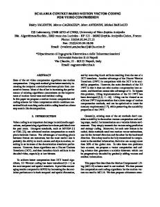
1) Predict step to generate the temporal high subband: The temporal high subband is temporally located at the odd frames X2t−1 . Using available motion vectors, the analysis equation is, √ ˜ 2t (m − dm , n − dn ) − X2t−1 (m, n)))/ 2, Ht (m, n) = (X (1) ˜ is the interpolated value at the subpixel location, where X using the method in [1] or any other. 2) Update step to generate the temporal high subband: The first step here is to reverse the forward motion field output from HVSBM to get the backward motion field as shown in Figure 2. For each pixel [m, n] in the current frame we find its match in the next frame using the forward motion vector (dm , dn ) and infer a backward motion field for pixel ([m + dm ], [n + dn ]) as (b[m+dm ] , b[n+dn] ) = −(dm , dn ). Note that for a subpixel motion field, [m + d m ] represents the nearest integer valued pixel location. For all the connected pixels in X2t , the update equation is, √ ˜ t (m − bm , n − bm ))/ 2. (2) Lt (m, n) = (X2t (m, n) + H For all the ’multi-connected’ pixels, we have multiple availability for the backward motion field. We choose the backward motion vector based on the order in which the pixels are processed [1]. For the remaining ’unconnected’ pixels, we use the original values in X 2t . C. MCTF for biorthogonal filters In this section, we present a lifting based MCTF framework using longer biorthogonal (LGT 5/3 and CDF 9/7) filters. 1) Lifting based MCTF for subpixel accurate motion field: The Haar filters only need motion vectors between frame pairs. With longer filters filters, we need to estimate a forward motion field for every consecutive frame and then either infer the backward field from the forward field, or actually estimate this backward motion field. The inference method is used here, thus we have twice the number of motion vectors of the Haar MCTF. For a subpixel accurate motion field as shown in Figure 3, the motion paths appear on a subpixel grid. The backward motion vectors, shown as dashed lines in this figure, are inferred from the closest forward vector. Using HVSBM we must generate d = (d m , dn ), the forward motion vector for each pixel in X t , where t is the frame index.

IEEE TRANSACTIONS ON CIRCUITS AND SYSTEMS FOR VIDEO TECHNOLOGY, VOL. X, NO. Y, MONTH 2005 t

3

b) Generation of temporal low subbands: We timereference the temporal low subbands to even time positions. The procedure can represented as: For t = 1, 2, · · · L2 , If C2t (m, n) = CONTINUE,

x

d b=−d

Lt (m, n) = X2t (m, n) + ˜ t+1 (m − dm , n − dn ) + H ˜ t (m − bm , n − bn )). 0.25(H

(5)

If C2t (m, n) = START, ˜ t+1 (m − dm , n − dn )). (6) Lt (m, n) = X2t (m, n) + 0.5(H X2t−1

Fig. 3.

X2t

X2t+1

If C2t (m, n) = END,

X2t+2

: Start

: Subpixel position

: Continue

: Multi−connected pixel

: Single

: Forward motion vector

: End

: Backward motion vector

˜ t (m − bm , n − bn )), Lt (m, n) = X2t (m, n) + 0.5(H and If C2t (m, n) = SINGLE, Lt (m, n) = X2t (m, n).

Subpixel forward motion and inferred backward motion vectors

For each pixel [m, n] in the current frame we find its match in the next frame and infer the backward motion field for nearestneighbor pixel ([m + d m ], [n + dn ]) as (b[m+dm ] , b[n+dn ] ) = −(dm , dn ). Then we use the forward motion vector for pixel ([m + dm ], [n + dn ]) to further extend this motion path. In the presence of multi-connected and unconnected pixels, each pixel in a GOP can be classified into one of the four classes: (a) START, (b) CONTINUE, (c) SINGLE, or (d) END based on its position on a given motion path. These four classes indicate availability of motion vectors that are (a) forward only, (b) bidirectional, (c) unavailable, or (d) backward only, respectively. For the ’multi-connected’ pixels, we have multiple options available for the backward motion vector and we make a decision based on the scan order. The ’unconnected’ pixels in the last frame of a GOP are classified as SINGLE. But for all the other ’unconnected’ pixels, we use the forward motion vector to identify them as in the START class. The CONTINUE class contains the pixels having a bi-directional motion match, which hopefully will constitute the majority. 2) Lifting based MCTF using LGT 5/3 filters: Once we classify all the pixels based on the presence of forward and/or backward motion vectors, we do the motion compensated filtering to generate the temporal high and low subbands. a) Generation of temporal high subbands: We place the temporal high subbands at odd positions. For LGT 5/3 filters, the above procedure can represented as: For t = 1, 2, · · · L2 , If C2t−1 (m, n) = CONTINUE, Ht (m, n) = X2t−1 (m, n) − ˜ 2t−2 (m − bm , n − bn )). ˜ 0.5(X2t (m − dm , n − dn ) + X

(3)

If C2t−1 (m, n) = START, ˜ 2t (m − dm , n − dn ). Ht (m, n) = X2t−1 (m, n) − X

(7)

(4)

(8)

3) Modifications for CDF 9/7 filters: For LGT 5/3 filters, we had only one predict and update step, but for CDF 9/7 filters the analysis/synthesis is carried out in 2 lifting steps. For connected pixels, each step is similar to that of the 5/3 filters, but making use of the lifting coefficients provided in [3]. D. Sliding window MCTF Thus far, we have considered processing MCTF one GOP at-a-time with symmetric extension of the motion trajectories at the boundaries. Even though such symmetric extension is often employed for perfect reconstruction, it produces a PSNR drop at the GOP boundaries especially at the starting frames where a temporal high subband is located, as shown below in Section II-G. A similar problem occured in block based image coding [17] and was handled using either odd length tiles or overlapping tiles. A similar approach was applied to non-motion-compensated MCTF by Xu et al [21]. Since we are using FIR filters, and feed-forward or open loop coding, we do not have to restrict ourselves to a finite GOP size. Instead we think of the GOP as infinite size and implement a ’sliding window’ filter. This allows us to use actual data inplace of a symmetric extension. This would mean we have to ’look ahead’ causing a certain amount of delay at the receiver. For the k level temporal analysis on a fixed size GOP, the minimun GOP size is N = 2 k frames. If we are using a 2M (k) + 1 tap filter at stage k, we need the future M (k) frames at each temporal level. Hence the longer the filter, the longer is the delay. For n levels of temporal resolution, this delay can be evaluated as D(n) =

n−1

2k M (k).

n=0

If we use a 5/3 filter at each stage, the coefficients M (k) equal 2 and we need 30 frames on either side of the sliding window for the 4 stage MCTF to completely avoid the need for boundary extension. If we use Haar filters at the last stage (M (n − 1) equals 0) and 5/3 filters for the first 3 stages, we can limit this additional delay to D(4) = 13 frames. If we use

IEEE TRANSACTIONS ON CIRCUITS AND SYSTEMS FOR VIDEO TECHNOLOGY, VOL. X, NO. Y, MONTH 2005 1

9

17

25

33

4

Flower Garden at 2048 Kbps 39

38

37

36

35

W1 W2

34 W3

33

W4 W5

32 Haar: 34.93 (0.74) dB 5/3: 35.42 (1.67) dB 9/7: 35.28 (1.54) dB

31

Fig. 4. Temporal Multi-resolution Pyramid using ’sliding window’ approach 30 t-H t-LH t-LLH

1:2 1:2

g1(n)

1:2

h1(n)

1:2 t_LLL

1:2

g3(n)

1:2

h3(n)

10

20

30

40

50

60

70

80

90

100

g2(n)

Fig. 6. PSNR performance for Flower Garden with quarter pixel accurate MC and four-stage (GOP of 16) temporal decomposition

h2 (n)

g : High pass synthesis filters h : Low pass synthesis filters

Fig. 5.

0

Three level temporal synthesis

a 9/7 filter at the first stage (M (1) equals 4), the delay D(4) will be 16 frames. Thus the total buffer size for a 5/3 filter is 42 and for a 9/7 filter is 48. Figure 4 shows a three-level multiresolution temporal pyramid. The solid blocks W1, W2, etc. represent the windows involved in temporal analysis and the dashed extensions show the needed data buffer. Thus while encoding the first 8 frames, we need the first 16 input frames and perform MCTF as per the algorithm specified in Section II-C.1. At the decoder, to reconstruct frames 1-8, we need to wait till we receive window W2 (delay D(3) = 8) and then do the synthesis. E. Filter based weighting of temporal subbands All the temporal subbands generated by the MCTF are then spatially analyzed and encoded using EZBC [1], [7]. The goal of EZBC is to reduce the average distortion in a given group of frames, by minimizing the summation of the distortion over all the subbands. This strategy works well for orthogonal filters [19], but the 5/3 filter has significant departures from orthogonality. It was shown that for such linear phase nonorthogonal filters banks, we need to properly scale the various subbands. Scaling coefficients were evaluated for the 2-D spatial subband/wavelet transform in [19]. We can use a similar procedure temporally. For illustrative purpose, consider the non-motion compensation 3-stage temporal analysis/synthesis case. The decoder is shown in Figure 5. At decoder each pixels in various temporal subbands are filtered with a distinct combination of ¯ and g¯ as reconstruction low pass and high pass filters (i.e. h shown in Figure 5. Thus we will have a separate weighting coefficient for t-H, t-LH, t-LLH and t-LLL subbands as listed below. These equations do not take into consideration the possibility of unconnected pixels, which amount to 10 − 15%

at the full frame rate. t − H : w 3 = 12 n | g¯3 [n] |2 , 2 ¯ t − LH : w2 = 14 n | (h3 (g¯2 ↑ 2))[n] | , 1 ¯ ¯ t − LLH : w1 = 8 n | (h3 (h2 ↑ 2) (g¯1 ↑ 4))[n] |2 , t − LLL : w1 = 18 n | (h¯3 (h¯2 ↑ 2) (h¯1 ↑ 4))[n] |2 . ¯ h[n/p], if n multiple of p ¯ ↑ p)[n] = Where, (h 0, otherwise F. Coding System The output of the four stage MC temporal analysis system comprises one t-LLLL frame, one t-LLLH frame, two tLLH frames, four t-LH frames and eight t-H frames. These temporal subbands are then decomposed spatially. After spatial decomposition, each of the spatiotemporal subbands is then coded using the embedded zero block coder (EZBC) [7]. This is then a sliding window EZBC coder, which we denote as SW-EZBC. The basic scalable MC-EZBC codec [1] consists of three parts: a pre-encoder, an extractor, and a decoder. The preencoder effectively generates a high bitrate video archive that accommodates a large range of sub-stream bit rates. All the motion vectors and temporal subbands at each temporal resolution are grouped together. The motion vectors are coded losslessly using an adaptive arithmetic coder [2]. The second part of the MC-EZBC coding system, the extractor, selectively truncates the bitstream at a variety of reduced spatial resolutions, frame rates, and quality levels. The decoder then reconstructs the video at any dyadic resolution or frame rate by simply decoding the portions of the codestream that contain the subbands corresponding to that resolution plus all the lower resolutions. G. Experimental Results In this section we compare performances of 3 filters (Haar, LGT 5/3, and CDF 9/7) used in an MCTF with both a fixed size GOP and sliding window. All the test sequences used for computer simulation are CIF (352×288) resolution and full frame rate is 30 fps.


Flower Garden at 2048 Kbps 39

5

Motion Compensation NO MC

Temporal Levels 1

NO MC

4

Quarter pixel accurate MC

1

Quarter pixel accurate MC

4

38

37

36

35

34

33 Haar: 34.93 (0.74) dB SW(5/3): 35.75 (1.27) dB SW(9/7): 35.58 (1.04) dB

32

31

0

10

20

30

40

50

60

70

80

90

100

Fig. 7. PSNR performance for Flower Garden using sliding window approach with quarter pixel accurate MC and 4-stage temporal decomposition

MCTF Scheme FixedGOP- Haar FixedGOP- 5/3 FixedGOP- 9/7 SW- 5/3 SW- 9/7 FixedGOP- Haar FixedGOP- 5/3 FixedGOP- 9/7 SW- 5/3 SW- 9/7 FixedGOP- Haar FixedGOP- 5/3 FixedGOP- 9/7 SW- 5/3 SW- 9/7 FixedGOP- Haar FixedGOP- 5/3 FixedGOP- 9/7 SW- 5/3 SW- 9/7

Avg. PSNR (dB) 26.36 27.04 27.25 27.21 27.45 27.04 27.30 27.62 27.96 28.27 28.81 29.39 28.79 29.42 28.74 34.93 35.42 35.28 35.75 35.58

TABLE I C OMPARISON OF PSNR PERFORMANCE FOR Flower Garden AT 2048 K BPS FOR MCTF WITH VARIOUS FILTERS

1) MCTF over a fixed sized GOP: In the case of quarterpixel accurate motion estimation, Figure 6 shows a PSNR plot for four-stage temporal analysis of Flower Garden at 2048 Kbps. The average PSNR and standard deviation are also listed in brackets. We see that both LGT 5/3 and CDF 9/7 filters give better average PSNR values than do Haar filters. But they both exhibit significant PSNR drop at the beginning of each GOP. This is mainly due to the symmetric extension which affects the end with the t-H band more than the other end [17]. 2) SW-MCTF : After using either LGT 5/3 or CDF 9/7 for the first stage of SW-MCTF, we can further extend it to 4 level temporal decomposition using the 5/3 filter at the second and third stage, using a Haar filter for the last stage. This limits the required buffer to 16 frames on either side. The PSNR plot with quarter pixel accurate MC is shown in Figure 7. The schemes SW(5/3) and SW(9/7) refer to use of 5/3 and 9/7 filters, respectively, for the first level of temporal analysis. We also employ the filter based scaling coefficients as discussed in Section II-E. We see that the PSNR plot is much more constant for the SW-MCTF except for the startup transient. We also noticed significant visual improvement at these boundary frames with the use of the sliding window approach. Table I summarizes the average PSNR performance for Flower Garden with various MCTF schemes. The table compares results for the case of no MC verses quarter pixel accurate MC, one MCTF stage verses four, and fixed-size GOP verses sliding window. For all the filter banks, the use of quarter pixel MC instead of no MC gives improvement of around 2 dB for one MCTF stage and around 7 dB for four MCTF stages. For the non-MC SW case, use of the CDF 9/7 filters at the first stage proves to be more effective. With quarter-pixel accurate MC, we have the presence of unconnected pixels, which amount to 10-15 % at the first temporal stage and this number almost doubles at lower temporal levels. This also reduces the average length of motion trajectories. As a result, the LGT 5/3 filters are more effective in handling

Rate (Kbps) 512 1024 2048

Scheme Haar SW Haar SW Haar SW

MV Rate (% of total) 21.21 38.77 10.60 19.39 5.30 9.69

Y(dB)

U(dB)

V(dB)

28.47 28.31 31.95 32.39 35.40 36.04

33.56 31.64 37.58 36.75 40.62 40.30

32.68 30.84 36.80 35.82 40.07 39.11

TABLE II AVERAGE PSNR FOR Mobile Calendar AT VARIOUS BIT RATES WITH QUARTER PIXEL MOTION FIELD AND FOUR STAGE TEMPORAL DECOMPOSITION

connected/unconnected pixels than are the CDF 9/7 filters. But for the non-MC case, four stage sliding window MCTF using the CDF 9/7 filters at first stage worked the best. Tables II and III give average PSNR results using quarter pixel accurate motion vectors for Mobile Calendar and Flower Garden, respectively. For these test sequences we found a significant improvement in PSNR at higher bit rates. Thus the longer filters help in increasing the coding gain. But they also require almost twice amount of motion information as do the Haar filters. This is the main cause of the PSNR deficit at low bit rates. 3) Effect of motion field accuracy: Figure 8 shows a RateDistortion plot for the luminance (Y) component of Flower Garden for integer, half, and quarter pixel accurate MCTF, respectively. Table IV gives the corresponding numerical PSNR values at 2048 Kbps. The results with the sliding window approach at integer and half pixel MCTF match the results with Haar at half and quarter pixel accuracy, respectively. Thus we can benefit by using lower MC accuracy, and hence save computation, when using a longer temporal filter. For an integer pixel accurate motion field, the lifting based MCTF approach is equivalent to forming motion trajectories


1024 2048


MV Rate (% of total) 30.12 53.61 15.06 26.80 7.53 13.40

Y(dB)

U(dB)

V(dB)

27.71 26.90 31.40 32.22 34.83 35.89

32.34 29.48 36.50 36.11 39.79 39.57

33.97 31.84 37.98 36.95 41.39 41.24

Flower Garden 36 Haar SW 34

32

PSNR(dB)

Rate (Kbps) 512

TABLE III

6

AVERAGE PSNR FOR Flower Garden AT VARIOUS BIT RATES WITH

30

28

QUARTER PIXEL MOTION FIELD AND FOUR STAGE TEMPORAL 26

DECOMPOSITION 24 200

400

600

800

1000

1200

1400

1600

1800

2000

2200

Rate(Kbps)

Half Quarter


Y(dB) 30.38 33.68 32.96 34.90 34.83 35.89

U(dB) 34.27 36.48 37.58 38.64 39.79 39.57

V(dB) 36.70 38.50 39.48 40.31 41.39 41.24

Gain in Y(dB) +3.30 +1.94 +1.06

(a) Flower Garden 36

34

Haar SW

32

PSNR(dB)

MV Accuracy Integer

TABLE IV

30

28

26

AVERAGE PSNR AT 2048 K BPS F LOWER G ARDEN (CIF, 240 FRAMES )

24

22 200

400

600

800

1000

1200

1400

1600

1800

2000

2200

Rate(Kbps)

(b) and doing temporal filtering along them. The backward and forward motion vectors both align with these motion trajectories and show biggest PSNR gain over the Haar filters. However for the subpixel accurate motion field, notice that the relative gain, compared with that of the Haar filter, reduces as we increase the motion vector accuracy. We think this is because the motion trajectories actually follow a subpixel grid, and hence we get only approximate alignment in this case.

Fig. 8. PSNR (dB) of Y component vs Rate for Flower Garden with (a) half and (b) quarter pixel accurate motion field

230

III. E FFICIENT MOTION VECTOR ESTIMATION AND

240

ENCODING

250

We have seen that the potential advantage of the longer filters is curtailed at low bit rates by the cost of the extra motion information. Here we look at efficient joint encoding of this motion data. Starting at the highest temporal resolution, we predict the inital motion vector at the next lower temporal resolution and further refine it using a smaller search range. This not only reduces the complexity of the motion search but also gives rise to a more uniform and true motion field. A standard coding of the motion vectors follows a fixed quadtree scanning order and codes the motion vector residuals along that path using an adaptive arithmetic coder (AAC)[1], [18]. We can improve the motion vector coding performance by employing a context based binary arithmetic coder (CABAC)[9]. Further, instead of encoding motion vector residuals along the quadtree based scanning path, we can also reduce the motion vector rate further by using neighboring motion blocks or blocks from the previous frame or from a lower temporal resolution.

260

A. Motion estimation directed by result at next higher temporal level In Section II-A.1, we discussed conventional hierarchical motion estimation that makes use of a spatial multiresolution

270

280

290

300

150

160

170

180

190

200

210

220

230

240

250

(a) 230

240

250

260

270

280

290

300

310 150

160

170

180

190

200

210

220

230

240

250

(b) Fig. 9. Motion field between two t-LLL subbands with a) S-HVSBM (the conventional HVSBM using spatial hierarchy) b) T-HVSBM (using temporal hierarchy)


pyramid for efficiency. We first generated a 3 level spatial pyramid for both the current and reference frame. Then the motion search starts at the lowest spatial resolution and using smaller refinements at higher spatial resolutions the final motion vectors are estimated [2]. This method is less complex than exhaustive search and generates a more uniform motion field. But as we go down to the lower temporal resolutions, i.e. lower frame rates, the distance between the current and reference frame doubles with each level. In this case, conventional HVSBM needs a higher search range to get the good motion vector match. This not only increases the search complexity, but can also lead to incorrect motion vector matches. Figure 9(a) shows the motion vector field between two t-LLL subbands for Mobile Calendar generated using conventional HVSBM and quarter pixel accurate motion field. These two frames are 8 frames apart and use of spatial hierarchy gives rise to a highly nonuniform motion field motion field. Such a non-uniform motion field increases the motion vector rate and hurts coding efficiency at low bit rates. Instead we can make use of the built-in temporal multiresolution pyramid to initiate the HVSBM motion estimation at lower temporal resolutions. We do the pixel-by-pixel vector addition of the two motion fields at the previous level and use it as starting point for the motion vector search for each 4 × 4 block. We can generally use a smaller refinement range to generate the motion field. Thus instead of using a spatial multiresolution pyramid as in conventional HVSBM, we use the temporal pyramid. The smaller refinement range used also gives rise to a more uniform motion field as shown in Figure 9(b) and can help in the coding the motion field. Table V presents the comparison of these two motion estimation approaches. S-HVSBM stands for the use of spatial multiresolution pyramid to perform the motion estimation as discussed in Section II-A.1. T-HVSBM stands for the new approach we discussed in this section. The T-HVSBM approach produces a more uniform and accurate motion field. This clearly helps in reducing the motion vector rate. The uniform motion field generated by T-HVSBM shows less visual artifacts especially for the low frame rate sequences. For S-HVSBM sequences, we use search range of ±4 at the lowest spatial resolution and use refinement range of ±1 at higher spatial resolutions. Thus at the first stage of temporal analysis the effective search range is ±22. As we move down the temporal pyramid, we double the search range at lowest spatial resolution, but still use the same refinement range. Thus the effective search range at the 3 lower temporal resolutions is ±38, ±70 and ±134. On the other hand, for T-HVSBM, the refinement range we use at the 3 lower temporal resolutions is ±8, ±16 and ±32. This greatly reduces the complexity of the motion vector search. B. Motion vector encoding The motion vector data consists of two parts: the motion vector segmentation map and the motion vectors. Due to the non-uniform block structure, it is necessary to transmit the motion vector segmentation map. A sample 64 × 64 parent block and its corresponding quad-tree segmentation

Sequence Scheme Mobile Calendar Flower Garden Foreman

7

MV Estimation

MV Rate (Kbps) 198.51 191.74 274.49 269.44 225.15 223.96 362.48 337.03

S-HVSBM T-HVSBM S-HVSBM T-HVSBM S-HVSBM T-HVSBM S-HVSBM T-HVSBM

Bus

YSNR (dB), Rate 512 1024 28.31 32.39 28.41 32.51 26.90 32.22 27.02 32.37 34.64 37.87 34.85 38.17 27.21 31.70 27.66 31.93

(Kbps) 2048 36.04 36.16 35.89 36.02 41.15 41.45 35.97 36.20

TABLE V M OTION VECTOR RATE AND PSNR OF Y COMPONENT WITH MOTION ESTIMATION METHOD USING SPATIAL AND TEMPORAL HIERARCHY

1

1 0

0

0

1

0 0

0

0

1 0

1

1

0 0

0 0

0 0 0

1 0

0 0

0

0

0

0

(a)

(b) Fig. 10.

Motion vector coding using AAC

map are shown in Figure 10, where a leaf or terminal node is represented as ’0’ while an intermediate node is represented as ’1’. For encoding motion vectors, the method follows a fixed scanning order at both encoder and decoder as shown in Figure 10. Instead of encoding the actual x and y components of the motion field, we used the motion vector differentials along this scanning path as illustrated in (9) and (10), where k represents the index of the current block in the scanning order. Then all the subpixel accurate MV residuals are converted into integer symbol values, where we indicate motion vector accuracy by 1/p: Ex (k) = (mvx (k) − mvx (k − 1)) × 2p ,

(9)

Ey (k) = (mvy (k) − mvy (k − 1)) × 2p ,

(10)

These symbols are then encoded using an adaptive arithmetic coder (AAC). In this process, we adaptively update the M-ary probability information at both encoder and decoder. The motion vector coding is lossless and any reduction in the entropy of the motion vector symbols to be encoded or more efficient arithmetic coding can help reduce the motion vector rate and will allow us more bits to encode the spatiotemporal


8

t x

C B A

Current Block

Previous Block in the scan order X2t−1

Blocks used for Spatial prediction

Fig. 11.

subbands. In the next 4 subsections, we will discuss the approaches for more efficient motion vector coding. 1) Use of CABAC for MV encoding: In the conventional scheme, we use M-ary adaptive arithmetic coding (AAC) [18]. It used one probability model for all the motion vector symbols in a given frame and updates it adaptively at the encoder and decoder. As the number of symbols increases, this scheme faces the ’zero frequency problem’ [9], i.e. even the unused symbols must be assigned some initial probability. This causes a mismatch in the actual and adaptively generated probability model and hurts the performance of the arithmetic coder. The majority of motion vector symbols are in the vicinity of zero and a large number of symbols are not used at all. Thus we need a coding scheme that can identify such low probability symbols and encode them more efficiently. Here we replace this M-ary arithmetic coding by a context based binary arithmetic coding (CABAC) scheme very similar to the one used for H.26L [9]. In the initial binarization step, each motion vector symbol is represented by a unique binary pattern using the simple unary codes (i.e. 0 is represented as ’0’, 1 as ’10’, 2 as ’110’ and so on). A binary arithmetic coding engine then follows this, and allows us to encode different bins with different models or use multiple models for some select bins. As shown in (11) and (12), the context used here is the average of the motion vector symbols for 2 neighboring blocks: topmost block on the left and leftmost block on the top (refer to Figure 11). abs(Mx (A)) + abs(Mx (C)) 2

X2t+1

X2t+2

: pixel in a given frame : subpixel position : actual motion vector estimated using HVSBM motion vector estimate from the previous frame

Illustration of spatial prediction for motion vectors

ctxx =

X2t

(11)

abs(My (A)) + abs(My (C)) (12) 2 If both neighbors are not available, as will be the case of blocks along the left and top frame edge, we use the block that is available. This context is same as the one used in [9]. With the employed quadtree scanning order, we will always have these three neighboring blocks available at both the encoder and decoder. The probability distribution of the motion vector symbols indicates that the vast majority of symbols are either 0, 1, or 2. So the first three bins need more attention

Fig. 12.

Illustration of temporal prediction

and we can use the neighboring blocks to guess whether the given bin is 0 or 1 and encode that bin using the appropriate probability model. The context selection scheme in [9] uses 3 models for bin 1, one for the remaining bins, and one for the sign bin. We modified this scheme to use an additional two models each for the next two bins. Here also, we check if the context is above a preselected threshold and use a different model then. This gives further reduction in the MV rate. We use one context model for all the remaining bins and one for the sign bit. Thus we end up with nine context models for each vector component. We can use multiple models for these bins. But the probability having large symbols is low and this can lead us to ’context dilution’ problems [9] i.e. we do not have sufficient symbols to adaptively build the accurate probability model. We get a reduction of almost 10 percent in the motion vector rate relative to AAC. This demonstrates the efficiency of adaptive binary encoding in comparison with the adaptive M-ary coder. 2) Encode spatial motion vector prediction: Consider the case of the block termed as ’current block’ in Figure 11. If we encode motion vector residuals along the quadtree scanning order (see Figure 10(b)), we will use the darkly shaded block for the prediction. But if the areas of rapidly changing motion, these two blocks may not have similar motion and it will not be the best candidate to predict motion of current block. Instead we can use the average MV of the 3 neighboring blocks A, B and C (see Figure 11) to predict current MV and encode the prediction errors, E x and Ey .

ctxy =

E(k) = 2p mv(k) − mv(A) + mv(B) + mv(C) ] (13) [2p × 3 Note that with our scanning order, we will always have these blocks available for prediction at both encoder and decoder, thus making this procedure reversible. 3) Encode temporal motion vector predictions from the previous frame: In the previous subsection, we looked at an


9

t x

EX2t = 2p × (mvX2t − d

: Pixel in given frame : Subpixel position

mvt−Lt ), 2

EX2t+1 = 2p × (mvX2t+1 − (mvt−Lt − mvX2t )),

(14) (15)

: Actual motion vector

: MV prediction from Lower temporal Resolution

X2t−1

X2t

Lt

Fig. 13.

X2t+1

X2t+2

L t+1

Illustration of MV prediction from lower temporal resolution

approach to utilize spatial correlation of the motion field for more efficient motion vector coding. Now we will discuss a method to use temporal dependency of the motion field. Here the basic assumption is a uniform motion field so that motion paths continue from one frame to the next. We encode the first frame using spatial prediction. For the following frames, we project the motion field of the previous frame along its motion paths and use that as a prediction for the MVs in current frame. This process is illustrated in Figure 12. The dotted lines represent the projected motion vectors from the previous frame. Then for the current frame, we average the predictions for given block and encode the prediction residuals. We can either use AAC or CABAC to encode these symbols. For the motion field at the lowest temporal level and the first two subbands at each temporal resolution, there is no previous frame available to predict the motion field. In this case, we use a spatial prediction from neighboring blocks. 4) Encode temporal motion vector predictions from the lower temporal resolution: In Section III-A, we discussed how we can utilize the motion field at a higher temporal resolution to initiate the motion estimation at a lower temporal resolution. The multiresolution MCTF is carried out from highest to lowest temporal resolution. But to maintain temporal scalability, the motion vectors are losslessly encoded from lowest to highest temporal resolution. Thus for a 4-level temporal multiresolution pyramid, we first encode the motion field between the two t-LLL subbands. Then we can make use of this field to encode the motion fields between the t-LL subbands. In general, we can utilize a motion field at a lower temporal level to predict the motion field at a given resolution and then encode the prediction residuals. We use the motion field between the L t and Lt+1 subbands to predict the motion field between frames X 2t ,X2t+1 and frames X2t+1 ,X2t+2 , as shown in (14) and (15).

Note that the subtraction operation shown in (15) refers to vector subtraction between the two motion fields. So this may encounter the presence of some unconnected pixels without any prediction. Then for each block we average out the prediction residuals of all the connected pixels present in that block. This operation is illustrated in Figure 13. The dotted lines represent the projected motion vectors from the lower temporal resolution. We can then use either AAC or CABAC to encode these symbols. 5) Experimental Results: Table VI shows the motion vector rate for four types of prediction methods to generate motion vector symbols to be encoded: differentials along the scanning order (Scan), spatial prediction from neighboring blocks (Spatial), temporal prediction from MVs of previous frame (Temporal) or prediction from lower temporal resolution (TempLevel). We use the new motion estimation scheme THVSBM discussed in Section III-A. We encode the motion field using AAC or CABAC. Use of CABAC instead of the AAC gives a reduction of around 10% in the motion vector rate. Use of spatial or one of the two types of temporal predictions (Temporal or TempLevel) with CABAC gives further reduction in the motion vector rate and improves PSNR results especially at low bit rates. For Bus, Mobile Calendar and Flower Garden, the temporal prediction works better than spatial, while for Foreman, spatial prediction works better. The scheme using temporal prediction from lower temporal resolution, gives the best result for all sequences except for Mobile Calendar. The scheme using temporal prediction works best when the motion field is uniform. At lower temporal resolution, time between frames gets doubled and the temporal predictions do not always work well. We can adaptively switch between spatial or temporal prediction for each block, but that requires transmission of extra motion information. But we can control this overhead by selecting the prediction scheme on a frame basis or a 64x64 block size basis. Comparing the results in Table VI with the ones presented by Turaga et al [15], our results show significant PSNR gains of 4-5 dB for Mobile Calendar and 1-2 dB for Foreman. This gain can be attributed to both the presence of the update step and the use of motion field with variable sized block. But the detailed HSVBM motion field also has higher motion vector rate compared to 16 × 16 fixed size block matching. IV. C ONCLUSION MCTF using LGT 5/3 or CDF 9/7 filters gives better coding results as compared to the 2-tap Haar filter. In the case of no motion compensation, the 9/7 filter shows the best results of the three filters, but in the presence of a subpixel accurate motion field, the 5/3 filters give better coding results. MCTF on a fixed size GOP requires some extension of the data on either end, which results in a PSNR drop at the GOP


Sequence

Mobile Calendar

Flower Garden

Foreman

Bus

Coding Scheme AAC CABAC CABAC CABAC CABAC AAC CABAC CABAC CABAC CABAC AAC CABAC CABAC CABAC CABAC AAC CABAC CABAC CABAC CABAC

MV symbol type Scan Scan Spatial Temporal TempLevel Scan Scan Spatial Temporal TempLevel Scan Scan Spatial Temporal TempLevel Scan Scan Spatial Temporal TempLevel

MV Rate (Kbps) 191.74 168.22 142.96 137.72 141.83 269.44 233.64 206.12 193.47 192.70 223.96 199.65 187.71 201.02 183.83 337.03 311.94 293.02 288.37 284.30

YSNR(dB) Rate(Kbps) 512 1024 28.17 32.49 28.72 32.64 29.05 32.71 29.16 32.76 29.11 32.72 27.02 32.37 27.73 32.56 28.17 32.69 28.41 32.74 28.42 32.75 34.85 38.17 35.15 38.35 35.19 38.39 35.14 38.34 35.23 38.40 27.66 31.93 28.05 32.07 28.29 32.20 28.33 32.21 28.41 32.24

TABLE VI M OTION VECTOR RATE AND PSNR OF Y COMPONENT USING AAC AND CABAC

boundaries, a problem that is avoided using the sliding window approach. The conventional HVSBM can result in a non-uniform motion field at lower temporal resolutions. Instead we can use the motion field at the higher temporal resolution to initiate the motion search at the current temporal resolution and then use a much smaller refinement to generate a more uniform and accurate final motion field estimate. Instead of encoding the MV residuals along the quadtree scanning path, we obtained improved performance using predictions from: (a) neighboring blocks, (b) previous frame at current temporal resolution, and/or (c) next lower temporal resolution. R EFERENCES [1] P. Chen, J. W. Woods, Improved MC-EZBC with quarter-pixel motion vectors, ISO/IEC JTC1/SC29/WG11, MPEG2022/8366, Fairfax, VA, May 2002. [2] S.-J. Choi and J. W. Woods,“Motion-compensated 3-D subband coding of video,” IEEE Transactions on Image Processing, vol: 8 , p:155 - 167, Feb. 1999. [3] I. Daubechies and W. Sweldens, “Factoring wavelet transforms into lifting steps,” J. Fourier Anal. Appl., vol. 4 (no. 3), pp. 247-269, 1998 [4] A. Golwelkar and J. W. Woods, Motion compensated temporal filtering using longer filters, ISO/IEC JTC1/SC29/WG11, MPEG2002/M9280, Awaji, Dec 2002. [5] A. Golwelkar and J. W. Woods, “Scalable video compression using longer motion compensated temporal filters,” Proc. SPIE VCIP vol. 5150, p. 1406-1416, Jun 2003, Lugano, Switzerland. [6] A. Golwelkar and J. W. Woods, Improved Motion Vector Coding for the Sliding Window (SW-) EZBC Video Coder, ISO/IEC JTC1/SC29/WG11, MPEG2002/M10415, Hawaii, Dec 2003. [7] S.-T. Hsiang and J. W. Woods, “ Embedded video coding using invertible motion compensated 3-D subband/wavelet filter bank ”, Signal Processing: Image Communication, vol. 16, no. 8, pp. 705-724. May 2001. [8] L. Luo, J. Li and S. Li and Z. Zhuang and Y.-Q. Zhang, ”Motion compensated lifting wavelet and its application in video coding,” IEEE Intl.Conf. on Multimedia and Expo (ICME 2001), Tokyo, Japan, Aug. 2001

10

[9] D. Marpe, H. Schwarz and T. Wiegand,“Context-based adaptive binary arithmetic coding in the H.264/AVC video compression standard,” IEEE Transactions on Circuits and Systems for Video Technology, vol: 13 , p:620 - 636, July 2003 [10] J.-R. Ohm, “Three-dimensional subband coding with motion compensation,” IEEE Trans. Image Processing, vol. 3, pp. 559-571, Sept. 1994. [11] B. Pesquet-Popescu and V. Bottreau, “Three-dimensional lifting schemes for motion compensated video compression,” Proc. ICASSP, p. 17931796, Salt Lake City, UT, May 2001. [12] A. Secker, D. Taubman, “Motion-compensated highly scalable video compression using an adaptive 3-D wavelet transform based on lifting,” Proc. ICIP, vol: 2, p. 1029 - 1032, 7-10 Oct. 2001, Thessaloniki, Greece [13] A. Secker, D. Taubman, “Lifting-based invertible motion adaptive transform (LIMAT) framework for highly scalable video compression,” IEEE Transactions on Image Processing, vol. 12 , p. 1530 - 1542, Dec. 2003. [14] D. S. Turagaa, M. van der Schaar and B. Pesquet-Popescu, “Differential Motion Vector Coding for Scalable Coding,” Proc. of SPIE, vol. 5022, p. 87-97, Jan 2003, Santa Clara, CA. [15] D. S. Turagaa, M. van der Schaar and B. Pesquet-Popescu, “Complexity Scalable Motion Compensated Wavelet Video Encoding,” IEEE Transactions on Circuits and Systems for Video Technology, vol. 15, p. 982 993, Aug. 2005. [16] M. Vetterli and D. Le Gall, “Perfect reconstruction FIR filter banks: some properties and factorizations,” IEEE Transactions on Acoustics, Speech, and Signal Processing, vol: 37, pp. 1057 - 1071, July 1989. [17] J. Wei, M. Pickering, M. Frater, J. Arnold, J. Boman and W. Zeng, “Boundary artefact reduction using odd tile length and the low pass first convention (OTLPF)”, Proc. SPIE conf. on Applications of Digital Image Processing, vol. 4472, p. 282-289, July 2001. [18] I. H. Witten, R. M. Neal, J. G. Cleary, “Arithmetic coding for data compression,” Communication of ACM, vol. 30, p.520-540, June 1987. [19] J. W. Woods and T. Naveen, “A filter based bit allocation scheme for subband compression of HDTV,” IEEE Trans. on Image Processing, vol. 1, p. 436-440, July 1992. [20] J. Xu, Z. Xiong, S. Li, and Y.-Q. Zhang, “Three-dimensional embedded subband coding with optimized truncation (3-D ESCOT),” J. Applied Computat. Harmonic Analysis, vol. 10, p. 290-315, May 2001. [21] J. Xu, Z. Xiong, S. Li, and Y.-Q. Zhang, “Memory-constrained 3D wavelet transforms for video coding without boundary effects,” IEEE Trans. Circuits Syst. Video Technol., vol. 10, p. 812-818, Sept. 2002.