Motion Estimation Using Point Cluster Method and Kalman Filter
M. Senesh A. Wolf1 e-mail:
[email protected] Biorobotics and Biomechanics Laboratory, Faculty of Mechanical Engineering, Technion-Israel Institute of Technology, Haifa 32000, Israel
The most frequently used method in a three dimensional human gait analysis involves placing markers on the skin of the analyzed segment. This introduces a significant artifact, which strongly influences the bone position and orientation and joint kinematic estimates. In this study, we tested and evaluated the effect of adding a Kalman filter procedure to the previously reported point cluster technique (PCT) in the estimation of a rigid body motion. We demonstrated the procedures by motion analysis of a compound planar pendulum from indirect opto-electronic measurements of markers attached to an elastic appendage that is restrained to slide along the rigid body long axis. The elastic frequency is close to the pendulum frequency, as in the biomechanical problem, where the soft tissue frequency content is similar to the actual movement of the bones. Comparison of the real pendulum angle to that obtained by several estimation procedures—PCT, Kalman filter followed by PCT, and low pass filter followed by PCT—enables evaluation of the accuracy of the procedures. When comparing the maximal amplitude, no effect was noted by adding the Kalman filter; however, a closer look at the signal revealed that the estimated angle based only on the PCT method was very noisy with fluctuation, while the estimated angle based on the Kalman filter followed by the PCT was a smooth signal. It was also noted that the instantaneous frequencies obtained from the estimated angle based on the PCT method is more dispersed than those obtained from the estimated angle based on Kalman filter followed by the PCT method. Addition of a Kalman filter to the PCT method in the estimation procedure of rigid body motion results in a smoother signal that better represents the real motion, with less signal distortion than when using a digital low pass filter. Furthermore, it can be concluded that adding a Kalman filter to the PCT procedure substantially reduces the dispersion of the maximal and minimal instantaneous frequencies. 关DOI: 10.1115/1.3116153兴 Keywords: rigid body estimation, Kalman filter, point cluster technique
1
Introduction
Reliable data representing the bone motion is essential for the complete understanding of the lower and upper extremity kinematics. Several researchers used markers mounted on the skeletal pins inserted into the bones to measure in vivo kinematics 关1–3兴. The trajectories of these markers are tracked to estimate the position, velocity, and acceleration of the markers and bones. While this approach generates a valid representation of the motion of the skeletal components of the joint, several characteristics of this method, in particular, its invasive nature, make it inappropriate for everyday clinical measurements. The most frequently noninvasive method for measuring human locomotion involves placing markers on the skin of the analyzed segment 关4兴. After markers are placed, opto-electronic systems composed of several high-frequency infrared cameras are used to capture the markers’ location in space as a function of time. Markers attached to the skin are unquestionably safer and easier to use than pin markers. However, estimation of the skeletal motion from the observed markers attached to the skin is significantly affected by the elasticity and nonlinear soft tissue deformation. These deformations result in erroneous calculation of the joint kinematic parameters 关4–10兴 共e.g., joint center and axis of rotation兲. Furthermore, because of its nature, the artifacts have frequency content similar to the actual bone movement. Therefore, unlike instrument error, it is difficult to reduce it by means of a frequency-based filtering technique 关6,11兴. The scope and clinical 1 Corresponding author. Contributed by the Bioengineering Division of ASME for publication in the JOURNAL OF BIOMECHANICAL ENGINEERING. Manuscript received August 20, 2007; final manuscript received September 14, 2008; published online April 13, 2009. Review conducted by Mark Redfern.
Journal of Biomechanical Engineering
relevance of the in vivo measurement of human motion would be substantially improved if reliable measurements of skeletal movement could be obtained from skin-based marker systems. Some human motion studies describe three-dimensional in vivo segment motions without taking into consideration the errors associated with nonrigid body movement and the lack of rigorous validation of the methods. Several investigators have described methods that were introduced to reduce errors associated with nonrigid segment movements. These techniques, in general, model the segment as a rigid body, and then apply various estimation algorithms to obtain an optimal estimate of the rigid body motion. Che’ze et al. 关10兴 proposed a so-called “solidification” procedure to address the marker cluster deformation. The method first identifies the subset of three markers forming the least perturbed triangle throughout the entire motion to define the rigid shape that best fits the time-varying triangle. This triangle is then fitted to each measured triangle using the standard single value decomposition 共SVD兲 algorithm to solve a least-squares positioning problem. This method did not improve the performance obtained using standard SVD algorithm 关12兴. Lu and O’Connor 关13兴 expanded on the rigid body model approach; rather than seeking optimal rigid body transformation on each segment individually, multiple constrained rigid body transforms are sought, modeling the hip, knee, and ankle as ball and socket joints. The assumption of a ball and socket joint is a limitation of this approach. Andriacchi et al. 关4兴 approached the segment pose estimation by considering a cluster of markers distributed on a segment, each with assigned weighting factor, which can be varied from sample to sample point cluster technique 共PCT兲. The idea is to adjust the weighting factor of each marker at each step to minimize the
Copyright © 2009 by ASME
MAY 2009, Vol. 131 / 051008-1
Downloaded 06 Jun 2011 to 132.68.54.35. Redistribution subject to ASME license or copyright; see http://www.asme.org/terms/Terms_Use.cfm
changes of the inertia tensor eigenvalues. While these methods have shown initial promise, they remain to be independently verified relative to bone kinematics. Another type of method is based on a nonlinear state space, using an extended Kalman filter 关7,14兴 and a biomechanical model of the human body. In these works, the distance between the measured markers’ trajectories, followed by a Kalman-filter procedure, and the corresponding trajectories in the biomechanical model, is minimized. The biomechanical model used was a simple rigid kinematic chain with an ideal ball in a socket human joint. Therefore, this method does not take into account the mechanical 共e.g., range of motion兲 and pathological 共e.g., lost of degree of freedom兲 characteristics and lacks general validation. The purpose of this study is to test and evaluate the effect of adding a Kalman-filter procedure to the previously reported PCT method in the estimation of a rigid body motion. Our research hypothesis is that adding a Kalman filter to the PCT method will result in a smoother signal that better represents the real motion. The methods were tested on a compound planar pendulum using indirect opto-electronic measurements of markers attached to an elastic appendage that is restrained to slide along the pendulum. Comparison of a measured rotation angle to that obtained by estimation procedures enables evaluation of the methods’ accuracy and the contribution of the Kalman filter to the accuracy of the estimation.
2
Methodology
2.1 PCT. The PCT method 关4兴 is based on a cluster of points uniformly distributed on each segment. Each point is assigned with an arbitrary weighting factor, which can be varied at each time step. The location of marker i in the global 共lab兲 coordinated system is measured and the center of mass of the points is calculated as a function of the weighting factor. Then, the inertia tensor I共t兲 for the discrete cluster points is calculated as a function of the weighting factor and of the location of all markers in the global coordinated system, which is located at the center of mass of the points. The eigenvectors E j of I共t兲 were used to form the transformation matrix R共t兲 as follows: R共t兲 = 共E共t兲1,E共t兲2,E共t兲3兲
nonlinear optimization operator in MATLAB™. The mass distribution was defined in terms of a single distribution parameter and calculated such that the point with the largest displacement from the rest position, in the local 共cluster兲 coordinate system, was assigned the lowest weighting factor. At each time step, the rotation matrix 共RG i 兲, which describes the rotation from the cluster system 共local system-i兲 to the global 共lab-G兲 system, was calculated. To calculate the segment’s screw angle in a local coordinate system, at each time step, the rotation matrix 共RG i 兲 was multiplied by the rotation matrix that describes the rotation from the global system to the local system in the rest 0 T 兲. The latter is equal to 共RG position 共RG 0 兲 , which was calculated in the minimization algorithm. 2.2 Kalman Approach to Kinematic Estimation. The Kalman filter is one of the most useful tools available today for estimating the state of a dynamical system in the presence of noise 关15兴. In the Kalman-filter theory, state variables are collected into a state vector x共t兲 and undergo dynamic changes through the state function s共x共t兲兲. For the Kalman filter to provide good working results, the state function of each variable should represent the true dynamics as accurately as possible. Avoiding a specific model for the dynamics of the motion, the more general formulation for the state function is the approach used in the field of numerical differentiation 关7,14,16兴. In this approach, a generic variable xk 苸 x can be associated with a Taylor series expansion as
冤 冥冤 xk共t + 1兲
1 ts ts2/2!
x共k1兲共t + 1兲
0 1
x共k2兲共t
+ 1兲
.
冤 冥
1
⌳i = 冑共i兲21 + 共i兲22 + 共i兲23
The difference between ⌳0 共the eigenvalues’ norm at rest position兲 and ⌳s 共the eigenvalues’ norm at ts兲 could be calculated in terms of n cluster points weighting factor for each time step. This difference was defined as a function F = 共⌳s − ⌳0兲2
共4兲
Minimization of F was solved numerically using unconstrained
.
.
. tsN−1/N − 1!
ts
ts2/2!
.
.
.
.
.
.
.
.
.
.
.
.
.
.
.
.
.
.
.
.
.
.
.
.
.
.
.
.
.
.
.
.
.
0 .
.
.
.
.
.
1
x共kN兲共t + 1兲
⫻
共2兲
共3兲
ts2/2!
.
共1兲
associated with each of these eigenvectors in an eigenvalue 共t兲 j , j = 1 , 2 , 3. The eigenvalues form a basis for an optimization technique since they should remain invariant if the segment moves as a rigid body. If nonrigid body movement occurs, the eigenvalues will change their value during movement. An algorithm was developed to minimize the eigenvalue changes by redistributing the weight factor at each time step. At each time step, the eigenvalues and the sum of squares of the three eigenvalues 共eigenvalues’ norm兲 were calculated as a function of the mass distribution:
.
.
=
冤 冥冤 冥 xk共t兲
nk,0共t兲
x共k1兲共t兲 x共k2兲共t兲
nk,1共t兲
. .
共d兲
冥
nk,2共t兲
+
. .
共5兲
.
.
j = 1,2,3
.
.
e共t兲 j,x
051008-2 / Vol. 131, MAY 2009
0 0
tsN/N!
.
.
.
It should be pointed out that the procedure does not always yield a “legal” rotation matrix 共Appendix兲. The three eigenvectors have the form E共t兲 j = e共t兲 j,y , e共t兲 j,z
ts
.
.
.
x共kN兲共t兲
nk,N共t兲
where xk , ts, and N are the dth derivatives of the variable, time sampling interval, and series expansion order, respectively. In the proposed study N was taken as N = 2. The noise in the model is the Taylor remainder 共higher-order derivatives兲: Qk共i, j兲 =
ts2N+3−i−j 2 共N + 1 − i兲 ! 共N + 1 − j兲 ! 共2N + 3 − i − j兲 k
共6兲
The value 2k was set up according to the frequency content of the signal and the sampling frequency 关16兴
2k =
¯ kts ¯ N+2 /4兲ts兲2 共共M k e 3ts
共7兲
¯ k and M are calculated from the measurement spectrum where 共harmonic analysis 关17兴兲 and are defined as the signal cutoff frequency and upper bound, respectively. Transactions of the ASME
Downloaded 06 Jun 2011 to 132.68.54.35. Redistribution subject to ASME license or copyright; see http://www.asme.org/terms/Terms_Use.cfm
Fig. 1 Experiment setup: „a… system setup, „b… sliding mass, „c… static part, and pendulum hinge
3
Experimental Analysis
1共b兲兲. The spring constant is 187.5 N/m 共obtained from dynamic analysis of the pendulum motion兲. The system’s total moment of inertia, estimated from the free vibration of the planar pendulum 共where the springs were not connected兲, is Itotal = 0.4278共kg m兲. Plotting the frequency backbone for both the pendulum angle and the slider vibration 共Figs. 2共a兲 and 2共b兲兲 reveals that the elastic frequency is close to the pendulum frequency, as in the biomechanical problem, where the soft tissue frequency content is similar to the actual movement of the bones. We note that the frequency backbone is obtained by plotting the instantaneous maximal 共minimal兲 amplitudes 共Amax/min兲 versus their corresponding maximal 共minimal兲 frequencies 共Fmax/min兲, where the last are calculated as the harmonic mean of the three opposite consecutive instantaneous periods: −1 −1 + Ti−1 + Ti+1 兲/3 F = 共Ti−1
3.1 Experiment Setup. The experimental system is composed of a planar pendulum 共M = 0.922 kg兲 on which an elastic appendage 共m = 2.05 kg兲 is restrained to slide along 共Figs. 1共a兲 and 1共b兲兲. The pendulum is mounted on a fixed base via a shaft and a bearing 共Fig. 1共c兲, solid line arrow兲. The shaft is free to rotate and is connected to an encoder 共Fig. 1共c兲, dashed line arrow兲 via a coupler 共Fig. 1共c兲, dotted line arrow兲. Four markers 共reflectors兲 were attached to the static 共rigid兲 part of the pendulum 共Fig. 1共c兲兲 and five markers were attached to the appendage 共Fig.
共8兲
During experiments, the pendulum was oscillating freely about the fixed base while the position of the markers was measured using the vicon motion capture system 共M ⫻ 13兲 关18兴. Four cameras were used and the pendulum was positioned in the center of the view of each camera. The reported capture system error is 0.1 pixel, which is equivalent to 0.1–0.2 mm 共in 3D兲 关18兴. 3.2 Experiment Results. In this section, we present the result of the angle calculation compared with the real angle. All data
Fig. 2 Frequency backbones: „a… pendulum and „b… slider mass
Fig. 3 Real angle: „a… static part of the pendulum and „b… pendulum hinge
Journal of Biomechanical Engineering
MAY 2009, Vol. 131 / 051008-3
Downloaded 06 Jun 2011 to 132.68.54.35. Redistribution subject to ASME license or copyright; see http://www.asme.org/terms/Terms_Use.cfm
Fig. 4 PCT estimated angle: „a… static part of the pendulum and „b… pendulum hinge
analysis was done using MATLAB™ 7.2. The cutoff frequency of = 13 Hz was evaluated using harmonic analysis 关17兴. However, in order to get enough noise reduction and less signal distortion, the cutoff frequency was set to ¯ k = 20 Hz. The signal upper bound was also set based on the harmonic analysis to M = 80 dB. Figures 3–5 describe the real angles, the PCT estimation angles, and the Kalman filter followed by the PCT estimation angles—of both the static part and pendulum hinge. Note that for both the static parts of the pendulum and the pendulum hinge, the estimation based on the Kalman filter followed by the PCT yields a less noisy signal compared with the estimation based only on the PCT method. 3.3 Accuracy of the Estimated Response. Several parameters were evaluated in order to compare the accuracy of the two presented methods. The first comparison is between the calculated maximal angular amplitudes 共Fig. 6兲. The maximal angular amplitudes were estimated as the maximal point of applied cubic spline interpolation on the measured/ estimated signal in the apex areas. A relative error between the maximal angular amplitudes was defined as
E% = 兩兩m兩 − 兩e兩兩/兩m兩 ⫻ 100%
共9兲
where m and e are the measured and estimated maximal angular amplitudes, respectively. Figure 7 shows that in both methods there is a variant error with a maximal value of ⬃4%. When comparing the maximal amplitude 共Figs. 6 and 7兲, one can conclude that no significant effect is noted by adding the Kalman filter; however, a closer look at the signal 共Fig. 8兲 reveals that the estimated angle based only on the PCT method is very noisy with fluctuation, and the estimated angle based on the Kalman filter followed by the PCT is a smooth signal. The second comparison is between the instantaneous maximal 共minimal兲 frequencies 共Eq. 共8兲兲. Note that the instantaneous frequencies obtained from the estimated angle based on the PCT method are more dispersed than those obtained from the estimated angle based on the Kalman filter followed by the PCT method 共Fig. 9兲. The dispersion of the data was estimated as
Fig. 5 Kalman filter followed by PCT estimated angle: „a… static part of the pendulum and „b… pendulum
051008-4 / Vol. 131, MAY 2009
Transactions of the ASME
Downloaded 06 Jun 2011 to 132.68.54.35. Redistribution subject to ASME license or copyright; see http://www.asme.org/terms/Terms_Use.cfm
冑兺 n
si =
共Fi − Fˆi兲2/共n − 2兲
共10兲
i=1
Fig. 6 Maximal angular amplitudes: „+… real angle, „䊊… PCT estimated angle, and „*… Kalman filter followed by PCT estimated angle
where Fi and Fˆi are the maximal/minimal instantaneous frequencies obtained from the estimated and real angles, respectively, and n is the number of measurements. A statistic test 共F test兲 has been conducted to determine if the difference in the dispersion is statistically significant. The F statistics for the maximal and minimal instantaneous frequencies are 19.73 and 18.34, respectively. Both results are much greater than the appropriate F critical 共Fcritical = 2.62兲 for 99% confidence interval. Therefore, it can be concluded that adding a Kalman filter to the PCT procedure substantially reduces the dispersion of the maximal and minimal instantaneous frequencies. The results were also compared with an estimated angle using a standard digital low pass filter 共Butterworth兲, which was reported to be used in biomechanics data analysis 关17兴, followed by the PCT algorithm. The low pass filter parameters are a function of a cutoff frequency, which was evaluated as previously described. The estimated angles are presented in Fig. 10. The relative error between the maximal angular amplitudes as defined in Eq. 共9兲 was also calculated for this procedure, and a two-sided pair t-test was conducted between the errors of the estimated angle based on the Kalman filter followed by the PCT and the errors of the estimated angle based on the low pass filter followed by the PCT. The test P value was 0.0166, which is statistically significant 共P ⬍ 0.05兲. Therefore, it can be concluded that the two relative errors have different mean values. The statistical parameter d was defined as d = EKalman − Elow pass and the calculated t parameter was ⫺2.451, which is much smaller than the lower 95% confidence boundary for this case 共⫺0.79077兲, meaning the mean relative error of the estimated angle based on the Kalman filter followed by the PCT is significantly smaller than the mean relative error of the estimated angle based on the low pass filter followed by the PCT. Note that when comparing the instantaneous frequency, there was no difference between the two methods.
4
Fig. 7 Relative error between the real and estimated angle: „䊊… Kalman filter followed by PCT estimated angle and „+… PCT estimated angle
Discussion and Closing Remarks
In this study, we tested and evaluated the effect of adding a Kalman-filter procedure to the previously reported PCT for the estimation of a rigid body motion. The analysis was carried out on an actual mechanical system and not by computer simulation only. The measurements were obtained using the vicon motion system, which is used in human gait analysis.
Fig. 8 Closer look at the signals: „ⴚ… real angle, „…… PCT estimated angle, and „--… Kalman filter followed by PCT estimated angle
Journal of Biomechanical Engineering
MAY 2009, Vol. 131 / 051008-5
Downloaded 06 Jun 2011 to 132.68.54.35. Redistribution subject to ASME license or copyright; see http://www.asme.org/terms/Terms_Use.cfm
Fig. 9 Instantaneous frequency: „a… instantaneous maximal frequency, „b… instantaneous minimal frequency. „䊊… real angle, „+… PCT estimated angle, and „*… Kalman filter followed by PCT estimated angle
The methods were tested on a compound planar pendulum using indirect opto-electronic measurements of markers attached to an elastic appendage that is restrained to slide along the pendulum. The elastic frequency 共of the elastic appendage兲 is closer to the pendulum frequency, as in the biomechanical problem, where the soft tissue frequency content is similar to the actual movement of the bones. In this simple dynamics system, the rigid rod 共pendulum兲 represents the bone, and the soft tissue is represented by the combination of the two springs and slider mass 共Fig. 11兲. The idea behind this dynamics system is the description of a soft tissue as a complex set of masses connected with springs. However, we chose to validate the procedure on the simplest system composed of one mass and two springs. Although this system does not completely simulate the mechanical properties of the human body, we used it since it allows to examine the effectiveness and accuracy of the proposed methods with respect to the true measurement of the rigid body motion, i.e., the pendulum motion. In actual human trials, this comparison cannot be carried out without the use of an invasive method 共or high exposure to radiation兲 to extract real bone motion. Comparing the maximal amplitude revealed no effect as a result of adding the Kalman filter. However, a closer look at the signal
revealed that the estimated angle based on only the PCT method was very noisy with fluctuation, while the estimated angle based on the Kalman filter followed by the PCT was a smooth signal. It should also be noted that in both the real angle and the estimated angle based on the Kalman filter followed by the PCT method, the cubic spline interpolation followed the actual signal; however, for the estimated angle based on the PCT method only, the interpolation was actually a smooth signal. Furthermore, it can be concluded that adding a Kalman filter to the PCT procedure substantially reduces the dispersion of the maximal and minimal instantaneous frequencies. The maximal and minimal instantaneous frequencies are indices for the signal phase; therefore, the angle estimation using the PCT leads to a time shift and signal phase inconsistency. The results of the estimated angle based on a digital low pass filter followed by the PCT method and the estimated angle based on a Kalman filter followed by the PCT method were compared. The relative error of the maximal amplitude in the Kalman filter followed by the PCT method was smaller than that in the low pass filter followed by the PCT method. This means that less signal distortion occurs when using a Kalman filter over a digital low pass filter. Future research will incorporate controlled human motion ex-
Fig. 10 Low pass filter followed by PCT estimated angle: „a… static part of the pendulum and „b… pendulum
051008-6 / Vol. 131, MAY 2009
Transactions of the ASME
Downloaded 06 Jun 2011 to 132.68.54.35. Redistribution subject to ASME license or copyright; see http://www.asme.org/terms/Terms_Use.cfm
The rotation matrix can be presented as three axes 共vectors兲 as follows: R共ts兲 = 关e共ts兲1
e共ts兲2
e共ts兲3兴
共A1兲
The first phenomenon occurs when the cross product of two axes does not yield the third axis. Therefore, for each time step, after the optimization algorithm is applied and a rotation matrix was calculated, three inequalities were examined as follows: 共ei ⫻ e j兲 − ek ⬍
共A2兲
where i ⫽ j ⫽ k have the values of 1, 2, and 3 for i = 1, and are permuted cyclically for i = 2 and i = 3. is set to a small value 共for this study it was chosen as = 0.001兲. In false cases, the direction of the third axis was rotated by 180 deg by ek = − ek
共A3兲
The correction of the second phenomenon, where two axes rotated by 180 deg, compared with the previous position, was done by examination of the below inequalities: ei−1 · ei ⬍ 0,
i = 1,2,3
共A4兲
In the case of a false sentence, the direction of the 共i兲 axis was rotated by 180 deg 共Eq. 共A3兲兲.
References
Fig. 11 The bone is represented by a rigid rod and the soft tissues are represented by a combination of springs and slider mass
periments when a subject will be asked to perform a simple planar motion with one segment, which will be fixed to an external device. Calculating the segment motion, using the presented methods, will be compared with a measured motion of the rigid external device.
Acknowledgment M.S. would like to thank the Diane and Leonard Sherman Interdisciplinary Graduate School Fellowship and the Gutwirth Fellowship.
Appendix Applying the PCT technique on the measurements of a rigid moving segment 共measured using optic-electromotion system兲 causes two undesirable phenomena: 共1兲 In several cases, the rotation matrix extracted from the inertia tensor had a determinate of ⫺1, which describes reflection instead of rotation. 共2兲 In several cases, the rotation matrix described the legal rotation matrix 共determinant equals to 1兲 but compared with the rotation matrix in the previous time step, two axes were rotated by 180 deg, which is not a reasonable incremental deformation. In order to correct the two undesirable phenomena, correction algorithms were introduced as follows.
Journal of Biomechanical Engineering
关1兴 Chan, M., 1993, Evaluation of the Use of Knee Braces Based on the Intrinsic Kinematics of a Normal Knee, MIT, Cambridge, MA. 关2兴 Lafortune, M. A., Cavanaugh, P. R., Sommer, H. J., and Kalenak, A., 1992, “Three-Dimensional Kinematics of the Human Knee During Walking,” J. Biomech., 25, pp. 347–357. 关3兴 Murphy, M. C., and Mann, R. W., 1991, “Estimation of the Instantaneous Kinematics of the Normal Human Knee In Vivo,” 37th Annual Meeting of the Orthopaedic Research Society, Anaheim, CA. 关4兴 Andriacchi, T. P., Alexander, E. J., Toney, M. K., Dyrby, C., and Sum, J., 1998, “A Point Cluster Method for In Vivo Motion Analysis: Applied to a Study of Knee Kinematics,” ASME J. Biomech. Eng., 120, pp. 743–749. 关5兴 Manal, K., McClay, I., Galinat, B., and Stanhope, S., 2003, “The Accuracy of Estimating Proximal Tibial Translation During Natural Cadence Walking: One vs. Skin Mounted Targets,” Clin. Biomech. 共Bristol, Avon兲, 18, pp. 126–131. 关6兴 Cappello, A., Stagni, R., Fantozzi, S., and Leardini, A., 2005, “Soft Tissue Artifact Compensation in Knee Kinematics by Double Anatomical Landmark Calibration: Performance of a Novel Method During Selected Motor Tasks,” IEEE Trans. Biomed. Eng., 52共6兲, pp. 992–998. 关7兴 Cerveri, P., Rabuffetti, M., Pedotti, V., and Ferrigno, G., 2003, “Real-Time Human Motion Estimation Using Biomechanical Models and Non-Linear State-Space Filters,” Med. Biol. Eng. Comput., 41, pp. 109–123. 关8兴 Reinschmidt, C., Van Den Bogert, A. J., Lundberg, A., Nigg, B. M., and Murphy, N., 1997, “Effect of Skin Movement on the Analysis of Skeletal Knee Joint Motion During Running,” J. Biomech., 30共7兲, pp. 729–732. 关9兴 Ryu, J. H., Kouchi, M., Mochimaru, M., and Lee, K. H., 2003, “Analysis of Skin Movements With Respect to Bone Motions Using MR Images,” International Journal of CAD/CAM, 3共2兲, pp. 61–66. 关10兴 Chèze, L., Fregly, B. J., and Dimnet, J., 1995, “A Solidification Procedure to Facilitate Kinematic Analysis Based on Video System Data,” J. Biomech., 28, pp. 879–884. 关11兴 Leardini, A., Chiari, L., Croce, U. D., and Cappozzo, A., 2005, “Human Movement Analysis Using Stereophotogrammetry—Part 3: Soft Tissue Artifact Assessment and Compensation,” Gait and Posture, 21, pp. 212–225. 关12兴 Vithani, A. R., and Gupta, K. C., 2004, “Estimation of Object Kinematics From Point Data,” J. Mech. Des., 126, pp. 16–21. 关13兴 Lu, T.-W., and O’Connor, J. J., 1999, “Bone Position Estimation From Skin Marker Co-Ordinates Using Global Optimisation With Joint Constraints,” J. Biomech., 32, pp. 129–134. 关14兴 Cerveri, P., Pedotti, A., and Ferrigno, G., 2004, “Non-Invasive Approach Towards the In Vivo Estimation of 3D Inter-Vertebral Movements: Methods and Preliminary Results,” Med. Eng. Phys., 26, pp. 841–853. 关15兴 Choset, H., Lynch, K. M., Hutchinson, S., Kantor, G., Burgard, W., Kavraki, L. E., and Thrun, S., 2005, “Kalman Filtering,” Principles of Robot Motion: Theory, Algorithms, and Implementation, Massachusetts Institute of Technology, Cambridge, MA, pp. 269–301. 关16兴 Fioretti, S., and Jetto, L., 1989, “Accurate Derivative Estimation From Noisy Data: A State-Space Approach,” Int. J. Syst. Sci., 20共1兲, pp. 33–53. 关17兴 David, A. W., 1930, Biomechanics and Motor Control of Human Movement, Wiley, New York, pp. 33–45. 关18兴 Vicon Motion Systems and Peak Performance Inc., 2007, http:// www.vicon.com.
MAY 2009, Vol. 131 / 051008-7
Downloaded 06 Jun 2011 to 132.68.54.35. Redistribution subject to ASME license or copyright; see http://www.asme.org/terms/Terms_Use.cfm