IEEE TRANSACTIONS ON INTELLIGENT TRANSPORTATION SYSTEMS, VOL. 6, NO. 1, MARCH 2005
113
Motion Generation and Adaptive Control Method of Automated Guided Vehicles in Road Following Lotfi Beji and Yasmina Bestaoui
Abstract—Dynamics of automated guided vehicles (AGVs) are described by a nonlinear nonholonomic model with two inputs: the rear axle torque and the steering angle torque. This model uses integrated longitudinal and lateral behavior. The first part of this paper is concerned with motion generation, taking into account kinodynamics and motor’s constraints. Usual kinematics constraints are not always sufficient to provide feasible trajectories; thus, we focus on velocity limitation and the motor’s current and slew rate constraints. Optimal velocity is determined for AGVs along a specified path with a known curvature. The main result concerns the realistic situation when the parameters of the model describing the movement of the vehicle are not well known. A nonlinear strategy is proposed to ensure control of the vehicle even if the knowledge of the AGV’s constant parameters is not perfect. The proof of the main result is based on the Lyapunov concept and the proposed results are illustrated by simulations and some comments. Index Terms—Automated guided vehicles (AGVs), longitudinal–lateral dynamics, motion generation, nonlinear adaptive control.
I. INTRODUCTION
T
HE STUDY of the automated guided vehicle (AGV) behavior and effect of the various design parameters when moving on the plane practically occupies a central place in the automobile theory. This paper addresses the problem of automated road following: automatic movement along a given path. While an automated vehicle travels at a relatively low speed, controlling it with only a kinematics model may work. However, as automated vehicles are designed to travel at higher speeds, dynamics modeling becomes important. An important characteristic of many of the studies concerning the automated vehicle modeling and control [3], [4], [17] is that they deal only with some simplified low-order linear models. These models are too simple for studying the integrated longitudinal and lateral dynamics. Traditionally, the nonlinear model is considered to be useful in a simulation environment, while the linear model is used for control design. We are interested in control design for an automated vehicle represented by a full-order nonlinear nonholonomic model. More precisely, in this paper we consider a rigid vehicle moving at a high nonconstant speed on a planar road. As the speed of this vehicle is not slow, the wheels must move with
Manuscript received July 8, 2002; revised August 25, 2003 and February 12, 2004. The Associate Editor for this paper was T. Fukuda. The authors are with the Laboratory of Complexe Systems (LSC), Sciences and Technologies Department, Evry University, Evry Cedex 91020, France (e-mail:
[email protected];
[email protected]). Digital Object Identifier 10.1109/TITS.2004.833758
suitable sideslip angles to generate cornering forces [7]. The interaction between longitudinal and transversal forces due to the tires as well as the nonlinear nature of these forces are taken into account. The presence of the suspension is neglected. Consequently, the roll and pitch angles are not considered here. However, the suspension design must be considered in the comfort analysis. As the car is supposed symmetrical with plane, a two-axle vehicle can be considered. respect to The wheels are assumed to be exactly parallel and to have the same radius and sideslip angle and, hence, to rotate at the same speed. In our analysis, as a single-track model of the vehicle will be considered, some simplification holds, as the model can be linearized, at least as far as the trigonometrical functions of the various angles. Hence, the single-track approach is best suited to linearized models and, therefore, to the linear control theory [7], [17]. However, with the realistic situation when the parameters of the model are not perfectly known and, in order to give a consistent estimation to the AGV’s parameters, a linear model will be secluded in this paper. For kinematics models, the stabilization problem has essentially been solved with two types of control laws: time-varying piecewise continuous control and time-varying continuous control. For dynamics models, based on the nonlinear couplings and the feedback linearization technique, Freund and Mayer [6] have used this principle to create a linear behavior that allows free pole placement for vehicle control. It is well known that this technique is sensitive to uncertainties. In [17], the vehicle equations are given in a simple form where the aerodynamic forces are not considered. The model given in [17] exhibits the form of Lorenz equations, which describe a liquid convection. Thus, the problem of studying the vehicle behavior is put into the same row with problems of hydrodynamics and the chaotic behavior of the car is outlined. Unfortunately, there are no regular and effective methods of stability analysis for the nonlinear model of an AGV, such as in the linear case. The Lyapunov method for the stability analysis of nonlinear systems can be useful in this situation. Previous works, such as [7] and [11], highlight the contribution of the internal variables such as the rotation angles and velocities of the wheels into dynamics model. In this paper, both the vehicle nonlinear kinematics and dynamics are integrated into the state–space formulation. As a first step, kinodynamics are integrated into motion generation, assuming that the path curvature is known. A path is , and its motion specified by its geometry , , where is the trajectory through a function is the total motion time. While extenlength of the path and sive work has focused on computing the geometric path [8], [9],
1524-9050/$20.00 © 2005 IEEE
114
IEEE TRANSACTIONS ON INTELLIGENT TRANSPORTATION SYSTEMS, VOL. 6, NO. 1, MARCH 2005
[13]–[15], little attention has been given to selecting the optimal motion. For the temporal part of the trajectory, most controllers currently use the trapezoidal speed profile. This method is suitable only for tracking straight lines with single-stage constant speed. Optimal velocity is determined along a specified path with a known curvature, such as a straight line, a circle arc, a clothoid, or a cubic spiral. Other paths could be used [2]. As a second step, an adaptive control method is proposed using integrated longitudinal and lateral dynamics. Some parameters of the dynamics are considered to be uncertain. Interest in the adaptive control of nonlinear systems was stimulated by major advances in the differential geometric theory of nonlinear feedback control. A thorough treatment of this theory was given by Kristic [10]. This paper is organized as follows. The modeling part of direct current (dc)-actuated vehicles is presented in Section II. Section III deals with motion generation that introduces the curvature of the path into the kinodynamics model. In Section IV, the proposed nonlinear adaptive-control scheme allows an estimation of the unknown vehicle’s parameters. Simulation results are introduced in Section V, while some conclusions are given in Section VI.
Fig. 1.
AGV parameterization.
the angular velocity, the following nonlinear sixth-order vehicle model is proposed: (1) (2) (3)
II. MODELING
(4)
A single-track model that includes the transverse and longitudinal AGV dynamics and neglects roll and pitch angles [6] is considered in this paper. The guidance system operates the steering wheel, causing some wheels to work with a sideslip and to generate lateral forces. These forces cause a change of attitude of the vehicle and then a sideslip of all wheels. The resulting forces bend the trajectory [6]. The important dynamical variables are the vehicle orientation (yaw angle), the longitudinal velocity , and the sideslip angle . In normal road conditions, particularly if radial tires are used, the sideslip angles become large only when approaching the limit lateral forces [16]. The actual position of the center of gravity is determined by the Cartesian coordinates and in the absolute position. The and represent the front and rear aerodynamic quantities side forces, respectively. The rear and front longitudinal forces and , respectively, result from the powertrain and brakes. . Let deThe front aerodynamic drag forces are defined by note the steering angle at the front wheels. The following constants are also used: vehicle mass , moment of inertia , and the distance between the front (rear) wheels and the vehicle’s center of gravity. For the study of the AGV interactions, a model that is able to simulate the behavior of the vehicle must be built. The difficulties encountered in such a task are so large that different approaches have been attempted and, until now, there is no standard driver model that can be used in general. As usual, the complexity of the model must be chosen in a way that is consistent with the aims of the study and the availability of significant input data. Our model is based on the balance of the forces acting on the vehicle in the longitudinal and lateral directions (the detail of the forces is given in Figs. 1 and 2), the torques and kinematic conditions. Using the conventional notations where denotes the linear velocity and
(5)
(6) (7) where is the Euclidean norm and , since this is a planar motion. The aerodynamic side force on the front and the aerodynamic side force on the rear wheel wheel are given by [6] (8) (9) while the front aerodynamic drag force is (10) The rear aerodynamic drag force is neglected with respect to the front one. The aerodynamic resistance coefficient , atmospheric denhave been insity, and the vehicle cross-sectional surface represents the characteristic curves of cluded. Here, the tires, with and , etc. The characteristic lines include the limitations and the descending behavior for high values in the argument [6]. As shown in Fig. 3, and are determined by the same characteristic line, describing the side-force values of the argument (arg). For small ), a linear relation of the side values of arg (smaller than force can be recognized. When values of arg are greater than , the side force decreases. More details are given in [6].
BEJI AND BESTAOUI: MOTION GENERATION AND ADAPTIVE CONTROL METHOD OF AGVS
115
Fig. 2. Diagram of the applied forces AGV.
Then, we combine (4), (6), and (11) to obtain (12). As we can and are eliminated and substituted see in these relations, by the rear wheels’ torque in order to simplify the tracking investigation [1]. (12) where and is the wheels radii. regroups the rear axle polar moment of inertia and the motor moment of inertia. is the front axle polar moment of inertia. The steering angle of the front wheel is the input for the vehicle in [6]. However, the real input of the guidance system is the torque/force applied to the steering wheel, thus giving a steering wheel angle resulting in the front wheel orientation. This is the basic idea of our control approach (13)
Fig. 3.
Characteristic curve of the tires [6].
There are three main sources of nonlinearities: the presence of products of the variables of motion in the equation, the presence of trigonometric functions, and the nonlinear nature of forces due to the tires. All of these nonlinearities are often neglected, such as in [6] and [7]. There, the steering angle and the sideslip angles of the wheels and of the vehicle are supposed to be very small. In our model, the interaction between longitudinal and lateral forces due to the tires is not neglected. Let us denote the control torque for the rear axle, which is given by (11)
is the torque for steering intervention, denotes the gear ratio, is the inertia moment, and is the viscous friction. Here, we exclude uses of differential brake and the two wheels’ are assumed to be identical. For vehicle steering intervention through differential braking, we can refer to Pilutti [12]. The handling of the vehicle can be studied by using these two equations. Aerodynamics forces are considered in this study; they introduce a strong dependence on . A similar, but far less important, effect is due to rolling resistance. The actuator of the steering column is an electric motor with a dc (available on certain standard vehicles). For a permanent magnet dc motor, the torque is proportional to the armature current . Thus, actuator dynamics can be characterized in a matrix form as (14)
116
IEEE TRANSACTIONS ON INTELLIGENT TRANSPORTATION SYSTEMS, VOL. 6, NO. 1, MARCH 2005
with with and . Further, , , are (2 2) regular diagonal matrices representing, reand spectively, the inductance, resistance, and torque constants of the actuators. is the motor voltage vector. We assume that the transmission from the motors to the mechanism is perfectly rigid, i.e., the transmission does not suffer from backlash or flexibility.
and
B. Problem Formulation
III. MOTION GENERATION A. Introduction of the Curvature of the Path Into the Kinodynamics Model As known from everyday experience, velocity depends on the curvature of the road. The higher the curvature, the lower the velocity, so the basic idea of this motion generation is to consider this relationship, not only in the kinematics layer but also in the dynamics layer. Let denote the vehicle curvilinear abscissa; . The orientation is given by then,
(15) while the curvature
with
may be obtained with
(16) When considering reference trajectories, we have to assume that the model is perfect and that the situation is ideal, so the dynamic model can be expressed as (1)–(8)
Designing reference trajectories essentially is an optimization problem. The minimum time trajectory generation has been solved in a number of ways, following the usual approach, i.e., taking purely kinematics constraints on vehicle velocity and acceleration as feasible limits. This bound must represent the global least upper bound of all operating accelerations so as to enable the vehicle to move under any operating conditions. This implies that the full capabilities of the vehicle cannot be utilized if the conventional approach is taken. In this paper, the case of more realistic constraints is investigated: current and slew rate constraints. In addition to current saturation, the guided vehicle also exhibits velocity saturation. This effect is due to back-electric motor force (emf) generation of the motors that, at high velocity, approaches the power supply voltage of the amplifier. The inclusion of slew rate limitations smoothes the change of rate of the current. The general problem of minimum time motion may be formulated as subject to Minimize total motion time (21) , , . and is the maximum velocity, is the current, repis the maximal slew resents the maximal current, and rate. The boundary values are given by , , , and . represents the maximum of the force provided by the motors. Following [5], the constraints on the currents or equivalently the torques can be transformed into constraints on the acceleration in the phase plane
(17) with
(22) where
(18) where the sideslip angle and velocity are null and the front longitudinal force is neglected. From a geometrical reasoning we can deduce that (19) For this conventionally driven vehicle, on a given path (in phase plane), using relations (15)–(19), the equations of motion are given by (20)
if if if
(23)
if if if
(24)
The maximum admissible velocity value is obtained when . This defines , taking into account the mechanical limitation on velocity. Resolution of these equations uses forward and backward integration. These equations allow us to construct an infeasible region in the state space ( , ) region for which the appropriate inputs for keeping the system on the path are not available. Equation (23) is used as an analysis tool only, verifying a posteriori that the calculated trajectories are admissible. The next paragraph proposes a practical method of resolution when the model is supposed to be perfect.
BEJI AND BESTAOUI: MOTION GENERATION AND ADAPTIVE CONTROL METHOD OF AGVS
C. Problem Resolution
117
and the vector
According to the Pontryagin maximum principle, a time optimal solution exists in which the input switches exclusively between the maximum and minimum, possibly zero during a finite interval (when the velocity is saturated). The terminal state requirement is a function of the switching interval lengths. If we suppose that the acceleration is constant during an interval, we can use the approximation
(29) The uncertainty constant dynamic parameters are regrouped in the following (7 1) vector:
(30) (25) For example, in the forward integration (26) The actual velocity depends on the past velocity, the path curvature, the motor current, and the vehicle parameters. When the equality of velocities [see (26)] that are computed with forward and backward integration is obtained, it is considered to be the switching time. Accelerations are obtained from (20). For each , the path curvature and its derivative are known. The characteristic of this motion-generation technique is that the curvilinear abscissa is the variable, while the time is a function of . Other suboptimal methods can be used, such as polynomial functions and sinusoidal curve to provide a higher degree of continuity.
We are interested in the unknown vehicle parameters (aerodynamic parameters and tire–road contact parameters). Parameters related to the dc motors can be obtained offline. The vehicle parameters should be written linearly in the model in order to use the adaptive control procedure. To show the dependence in the constant parameters, we write the dynamics of the vehicle as (31) which takes the compact form (32) The form of
is
IV. ADAPTIVE CONTROL METHOD Interest in adaptive control of nonlinear systems was stimulated by major advances in the differential geometric theory of nonlinear feedback control. A thorough treatment of this theory was given by Kristic [10]. The control problem formulated here consists of finding a control law to achieve tracking of a reference trajectory in task space with constant parametric uncertainties of the vehicle. In fact, it is not easy to measure some physical parameters such as aerodynamics parameters, parameters of the characteristic line describing the side-force values in the longitudinal and lateral directions, and frictions and moment of inertia of the steering wheel around the center of gravity. We rewrite the vehicle kinodynamics model combined with actuators dynamics such that the model is linear in the updated parameters and suitable for the control. We start with the following system (27), which was obtained from (12) and (13).
(27) , , , and where denotes the input in armature’voltages. Further, , and are functions of the dc motor parameters [1] , , and . The (2 constant inertia matrix is as
. , 2)
(28)
(33)
denotes the error in torques, which can be viewed as a perturbation to the dynamic of the vehicle. is a suitable desired torque that will be specified in the following. is generated by the dynamic of the Note that by using (27), actuators (34) The aim of the control is to specify , which should guarantee , as (time). Of course, from (27) we can take as input, but the internal dynamics due to actuators will be ignored. For an automatically guided mechanism, this hypothesis will be inherent to the displacement stabilities. Internal dynamics produce an error that should be rejected before tackling the stabilization-tracking problem. Therefore, our case for guided vehicle control in road following takes into account the actuators dynamic. Then, the voltage is taken as a control vector. , In the following, let us define the tracking error by , is a specified curvilinear abscissa, and where is the desired steering angle. , is the estimation with . of . We introduce
118
IEEE TRANSACTIONS ON INTELLIGENT TRANSPORTATION SYSTEMS, VOL. 6, NO. 1, MARCH 2005
Lemma 1: The open-loop system dynamics represented by is the state
Now, the input in voltages can be substituted to obtain the dynamic of the error in torques , which leads to (42)
(35)
Proof: First, we consider that the parameters of the guided vehicle are constant. Then, we can take . To prove the and let second line of (35) as , then with is given by (31). As we can see, the input of is , which will be specified in the following. Now, the fourth line in (35) is that given by (34) with . is an appropriate adaptive law that should ensure the vehicle stabilities even if the knowledge of parameters is not perfect. Lemma 2: Under the following control laws in torques: (36)
In the following, we need to compute the term in (42). From (32) and (36), we have (43) Then, clearly, we get (44) Substituting (44) into (42), it is straightforward to verify that where , which is an exponentially stable dynamic. Our stability results are formulated in the following theorem. Theorem 1: The parametric model of the dc-actuated longitudinal–lateral automatically guided vehicle given by (32) and (34) is
and in voltages (45) with , , dynamics of the system in the closed loop is given by
(37) , the
(46) (38)
where
having as inputs and , given by (36) and (37), respectively, and the update law for
is asymptotically stable. Then, as . . and as . Moreover, Proof: The candidate such as the Lyapunov function is
is obtained from (33) as (47) Note that depends only on , so its time derivative is is given by equal to zero. Therefore, the time derivative of (39)
(48) which takes this form (49) (50)
and
. , , , ) Proof: Note that the origin ( is an equilibrium of (38). The dynamic, as function of the estimated parameters, is considered in (40) Now, the dynamic in the closed loop of is the subject of the substitution of by in (35), which leads to
(41) Then, the state
in the closed loop is verified.
Some simplifications permit us to write (51) which is negative definite, meaning that the origin ( , , , and ) is an asymptotically stable equilibrium point ( as ). V. SIMULATION RESULTS Many simulations were performed with a vehicle whose characteristics are [7] kg, kgm , m, m. and , , Both motors are identical: Nm/A, , , , and ms kmh . The reference trajectory is calculated using the approach presented in Section III. We suppose that we have no knowledge of the aerodynamic parameters and the front and rear road–tire
BEJI AND BESTAOUI: MOTION GENERATION AND ADAPTIVE CONTROL METHOD OF AGVS
119
Fig. 4. Straight-line path following for the AGV.
contact parameters. The length of the path is 10 m. Three cases are presented, as follows: • straight line, the curvature (Fig. 4); (Fig. 5); • arc of the circle, the curvature (Fig. 6). • clothoid, the curvature The guided vehicle control block diagram is shown by Fig. 7, while details about the model state variables are given in
Table II. The simulations are performed using MATLAB , , software and the initial conditions are , and . The performance of the tracking controller with the update control law is subject to following a straight line and an arc of circle curvatures. In this case, the parameters of the regulator , , , are chosen as
120
IEEE TRANSACTIONS ON INTELLIGENT TRANSPORTATION SYSTEMS, VOL. 6, NO. 1, MARCH 2005
Fig. 5. Circular path following for the AGV.
, and . is the (2 2) identity matrix. However, to follow a clothoid path, we adjust the following gain and . parameters of the controller: In each figure, 12 schemes appear, as follows: • • • • •
path ( versus ), the eleven left are all versus the time; position errors ( ; ); reference and real vehicle velocities on the path ( , ); reference and real vehicle accelerations on the path ( , ); reference and real jerks ( , );
voltage of the motors ; variation of the angle of the direction ( , ); reference and real angular velocities ( , ); longitudinal reference torque lateral reference torque ; variation of the three estimated parameters ( , ); • derivative of these three estimated parameters ( , ).
• • • • • •
, and , and
BEJI AND BESTAOUI: MOTION GENERATION AND ADAPTIVE CONTROL METHOD OF AGVS
121
Fig. 6. Clothoid path following for the AGV.
For the three cases of the road curvature, we obtain the following results for the estimated seven parameters. The values given in brackets (see Table I) follow the variation of the gain controller, which is in order to ensure the tracking performance of the clothoid path. When we have taken the gain controller identical for all these curvatures, only varies. As results, the aerodynamic coefficients and the rear road–tire contact parameters seem to be constant versus the curvature of the road, while the front road–tire contact parameter is greatly dependent on the
curvature of the road. As we can see, the parameter , which denotes the aerodynamic parameters, is important in the absolute value for the clothoid path. This parameter depends on the form of the path. More suitable investigation should be made while introducing the real tests on the vehicle. The input in voltages remains limited to 100 V, which guarantees the physical limitations of the actuators. The performance of the proposed adaptive controller is demonstrated where we show that the tracking and converge to zero for a finite value of errors
122
IEEE TRANSACTIONS ON INTELLIGENT TRANSPORTATION SYSTEMS, VOL. 6, NO. 1, MARCH 2005
Fig. 7. Guided vehicle control block diagram. TABLE I VEHICLE ESTIMATED PARAMETERS
TABLE II AGV’S MODEL STATE VARIABLES
time. The effectiveness of the controller, as well as of the update law, are illustrated on the other results of simulation. The proposed adaptive control law ensures the control of the vehicle even if the knowledge of its parameters is not perfect. This is
very useful insofar as certain parameters can be added with the law of adaptation. The procedure of adaptation should be more investigated for the characteristic curve of the tires, which are time-varying parameters.
BEJI AND BESTAOUI: MOTION GENERATION AND ADAPTIVE CONTROL METHOD OF AGVS
VI. CONCLUSION The first part of this paper has presented a vehicle dynamic model that is suitable for path planning and control studies. The second part proposed a method for generating smooth optimal motion for AGV on a given path when kinematics and dynamics constraints are taken into account. In specifying such a trajectory, the physical limits, such as velocity, current, and slew rate limits, were considered. In the third part of this paper, we have used an adaptive Lyapunov approach to propose a controller. Simulation processes lead to constant aerodynamic coefficients and rear road–tire contact parameters versus the curvature of the road. While the front road–tire contact parameter is greatly dependent on the curvature of the road. Although dc motors have been considered, other actuators such as alternating current (ac) machines present the same kind of constraints on both the current and voltage. Interesting applications of Hamiltonian methods, such as the energy-momentum method (for determining nonlinear stability) and bifurcation of Hamiltonian systems with symmetry (for uncovering non trivial branches of new solutions when system parameters such as friction coefficients are varied) are also a new perspectives. Other studies should be conducted about deformability or flexibility of the wheels, uneven roads, etc. ACKNOWLEDGMENT The authors would like to thank the anonymous reviewers and the Editor for their helpful revision of the manuscript. REFERENCES [1] L. Beji and Y. Bestaoui, “An adaptive control method of automated vehicles with integrated longitudinal and lateral dynamics in road following,” in Proc. Robot Motion Control (ROMOCO), Poland, 2001, pp. 201–206. [2] Y. Bestaoui, “An optimal velocity generation of a rear wheel drive tricycle along a specified path,” in Proc. American Control Conf. (ACC ), 2000, pp. 2907–2911. [3] C. Y. Chan, “Open-loop trajectory design for longitudinal vehicle maneuvers: Case studies with design constraints,” in Proc. American Control Conf. (ACC), 1995, pp. 4091–4095. [4] S. B. Choi, “The design of a control coupled observer for the longitudinal control of autonomous vehicles,” J. Dynam. Syst. Meas. Control, vol. 120, pp. 288–289, 1998. [5] O. Dahl and L. Nieslon, “Torque-limited path following by on-line trajectory time scaling,” IEEE Trans. Robot. Automat., vol. 6, pp. 554–561, Oct. 1990. [6] E. Freund and R. Mayer, “Non linear path control in automated vehicle guidance,” IEEE Trans. Robot. Automat., vol. 13, pp. 49–60, Feb. 1997. [7] G. Genta, Motor Vehicle Dynamics: Modeling and Simulation. Singapore: World Scientific, 1997. [8] H. Hu, M. Brady, and P. Probert, “Trajectory planning and optimal tracking for an industrial mobile robot,” in Proc. SPIE, vol. 2058, Boston, MA, 1993, pp. 152–163.
123
[9] Y. Kanayama and B. I. Hartmann, “Smooth local path planning for autonomous vehicles,” in Autonomous Robot Vehicles, I. J. Cox and G. T. Wilfong, Eds. New York: Springer-Verlag, 1990, pp. 62–67. [10] M. Kristic et al., Nonlinear and Adaptive Control Design. New York: Wiley, 1995. [11] R. Outbib and A. Rachid, “Control of vehicle speed: a non linear approach,” in Proc. Conf. Decision Control (CDC), Australia, 2000. [12] T. Pilutti et al., “Vehicle steering intervention through differential braking,” Trans. ASME, vol. 120, pp. 314–321, 1998. [13] V. Munoz, A. Ollero, M. Prado, and A. Simon, “Mobile robot trajectory planning with dynamic and kinematic constraints,” in Proc. Int. Conf. Robot. Automat. (ICAR), 1994, pp. 2802–2807. [14] D. B. Reister and F. G. Pin, “Time-optimal trajectories for mobile robots with two independently driven wheels,” Int. J. Robot. Res., vol. 13, no. 1, pp. 38–54, 1994. [15] N. Sadeghi and B. Driessen, “Minimum time trajectory learning,” in Proc. Amer. Control Conf. (ACC), 1995, pp. 1350–1354. [16] R. S. Sharp et al., “A mathematical model for driver steering control, with design, tuning and performance results,” Veh. Syst. Dynam., vol. 33, no. 5, pp. 289–326, 2000. [17] P. A. Shavrin, “On a chaotic behavior of the car,” in Proc. Eur. Control Conf. (ECC), 2001, pp. 2187–2192.
Lotfi Beji received the Dipl.-Ing. degree in electromechanical engineering from the Ecole National d’Ingénieur de Tunis, Tunis, Tunisia, in 1992 and the Dr.-Ing. degree from the Université d’Evry, Evry, France, in 1997. He was an Associate Professor with the Sciences Technologies in Engineering Department and the Laboratory of Complexe Systems Centre National de Recherche Scientifique-FRE2494. For his thesis, he worked in the modeling and control of parallel robots. He was invited by the Tunisian Minister of Research to work in the control of complex systems in the LIM Polytechnic Laboratory in Tunisia for six months in 2004. He is currently with the LSC Laboratory, Université d’Evry. His research interests have included the control of vehicles and blimps modeling and the identification and control of autonomous robots, including underactuated systems with holonomic and nonholonomic constraints.
Yasmina Bestaoui received the Ph.D. degree in automatic control from the Ecole Nationale Supérieure de Mécanique, University of Nantes, Nantes, France, in 1989 and the Habilitation to Direct Research (HDR) from the Université d’Evry, Evry, France, in 2000. From 1989 to 1999, she was an Assistant Professor and then an Associate Professor in the Mechanical Engineering Department, University of Nantes. She spent her sabbatical leave (October 1997–July 1998) in the Computer Science Department, Naval Postgraduate School, Monterey, CA. In 1999, she joined the Department of Electrical Engineering, Université d’Evry. For nine years, she had worked on robots manipulators, until 1998. Her actual research interests include trajectory generation and control of autonomous vehicles, both terrestrial and aerial.