moving object detection in 2d and 3d scenes a thesis ... - CiteSeerX

MOVING OBJECT DETECTION IN 2D AND 3D SCENES

A THESIS SUBMITTED TO THE GRADUATE SCHOOL OF NATURAL AND APPLIED SCIENCES OF MIDDLE EAST TECHNICAL UNIVERSITY

BY

SALİM SIRTKAYA

IN PARTIAL FULFILLMENT OF THE REQUIREMENTS FOR THE DEGREE OF MASTER OF THESIS IN ELECTRICAL AND ELECTRONICS ENGINEERING

SEPTEMBER 2004

Approval of the Graduate School of Natural and Applied Sciences

______________________ Prof. Dr. Canan Özgen Director I certify that this thesis satisfies all the requirements as a thesis for the degree of Master of Science. ______________________ Prof. Dr. Mübeccel Demirekler Head of Department This is to certify that we have read this thesis and that in our opinion it is fully adequate, in scope and quality, as a thesis for the degree of Master of Science. ______________________ Assoc. Prof. Dr. Aydın Alatan Supervisor

Examining Committee Members

Prof. Dr. Mübeccel Demirekler

(METU, EE)______________________

Assoc. Prof. Dr. Aydın Alatan

(METU, EE)______________________

Prof. Dr. Kemal Leblebicioğlu

(METU, EE)______________________

Assoc. Prof. Dr. Gözde Bozdağı Akar

(METU, EE)______________________

Assoc. Prof. Dr. Yasemin Yardımcı

(METU, IS)______________________

ii

I hereby declare that all information in this document has been obtained and presented in accordance with academic rules and ethical conduct. I also declare that, as required by these rules and conduct, I have fully cited and referenced all material and results that are not original to this work.

Salim SIRTKAYA

ABSTRACT

MOVING OBJECT DETECTION IN 2D AND 3D SCENES

Sırtkaya, Salim M.S., Department of Electrical and Electronics Engineering Supervisor: Assoc. Prof. Dr. Aydın Alatan

September 2004, 88 Pages

This thesis describes the theoretical bases, development and testing of an integrated moving object detection framework in 2D and 3D scenes. The detection problem is analyzed in stationary and non-stationary camera sequences and different algorithms are developed for each case. Two methods are proposed in stationary camera sequences: background extraction followed by differencing and thresholding, and motion detection using optical flow field calculated by “KanadeLucas Feature Tracker”. For non-stationary camera sequences, different algorithms are developed based on the scene structure and camera motion characteristics. In planar scenes where the scene is flat or distant from the camera and/or when camera makes rotations only, a method is proposed that uses 2D parametric registration based on affine parameters of the dominant plane for independently moving object detection. A modified version of the 2D parametric registration approach is used when the scene is not planar but consists of a few number of planes at different depths, and camera makes translational motion. Optical flow field segmentation and sequential registration are the key points for this case. For iv

3D scenes, where the depth variation within the scene is high, a parallax rigidity based approach is developed for moving object detection. All these algorithms are integrated to form a unified independently moving object detector that works in stationary and non-stationary camera sequences and with different scene and camera motion structures. Optical flow field estimation and segmentation is used for this purpose.

Keywords: Background Extraction, Optical Flow Field, Structure from Motion, Affine Parameter Estimation, Parallax Rigidity

v

ÖZ

2 BOYUTLU VE 3 BOYUTLU SAHNELERDE HAREKETLİ NESNE TESPİTİ

Sırtkaya, Salim Yüksek Lisans, Elektrik ve Elektronik Mühendisliği Bölümü Tez Yöneticisi: Doç.Dr. Aydın Alatan

Eylül 2004, 88 Sayfa

Bu tez, 2 boyutlu ve 3 boyutlu sahnelerde tümleşik hareketli hedef tespiti çözüm

iskeletinin

kuramsal

taban,

geliştirme

ve

test

etme

aşamalarını

anlatmaktadır. Tespit problemi, sabit ve hareketli kamera sahnelerinde tahlil edilmiş ve her iki durum için ayrı algoritmalar geliştirilmiştir. Sabit kamera sahneleri için iki ayrı yöntem sunulmuştur: Arkaplan özütlemeyi takip eden çıkarım eşikleme, ve “Kanade-Lucas Öznitelik İzleme” tekniği ile hesaplanan ışıl akış alanından hareket tespiti. Hareketli kamera sahneleri için sahne yapısı ve kamera hareket tipine bağlı olarak değişik algoritmalar geliştirilmiştir. Kameradan uzakta veya yassı olan düzlemsel sahnelerde ve/veya kamera sadece dönüş hareketi yaptığında, bağımsız hareket eden nesne tespiti baskın düzlemin ilgin parametrelerine dayalı 2 boyutlu parametrik çakıştırma yöntemiyle yapılmıştır. Sahnenin bir yerine birkaç düzlemden oluştuğu ve kameranın ötelenme hareketi yaptığı durumlarda, parametrik çakıştırma yönteminin değiştirilmiş bir sürümü kullanılmıştır. Bu durumda, ışıl akış alanı kesimlemesi ve ardışık çakıştırma anahtar noktalardır. vi

Derinlik değişiminin fazla olduğu 3 boyutlu sahneler için, parallaks sabitliği tabanlı bir yöntem geliştirilmiştir. 2 boyutlu parametrik çakıştırma bu yöntemde de kameranın dönüş hareketi ve optik kaydırmadan kaynaklanan etkileri ortadan kaldırmak için kullanılmaktadır. Tüm bu algoritmalar, sabit, hareketli kamera ve değişik sahne yapısı ve kamera hareket tipleri ile çalışabilecek, tümleşik bağımsız hareket eden nesne tespiti yapabilmek için birleştirilmişlerdir.

Anahtar Kelimeler: Arkaplan Özütleme, Işıl Akış Alanı, Hareketten Yapı, İlgin Parametre Kestirimi, Parallaks Sabitliği.

vii

ACKNOWLEDGEMENTS

I would like to express my sincere appreciation to my supervisor Assoc. Prof. Dr. Aydın Alatan for his continued guidance, also patience and support throughout my research. He provided counsel, and assistance that greatly enhanced my studies and know-how. I am also grateful to Tuba M. Bayık for her support, patience and belief in me. She consistently assisted and motivated me during the whole master’s period. Thanks go to my manager Dr. Murat Eren for his patience and support from beginning to end of my M.Sc. program. I am also grateful to several of my colleagues, especially those who shared my office and thereby my problems. These include Naci Orhan, Onur Güner, Alper Öztürk and Volkan Nalbantoğlu. And my parents and sisters, I want to thank them for everything. ASELSAN A.Ş. who supported this work is greatly acknowledged.

viii

TABLE OF CONTENTS

ABSTRACT .......................................................................................................... iv ÖZ…… ................................................................................................................. vi ACKNOWLEDGEMENTS....................................................................................viii TABLE OF CONTENTS ....................................................................................... ix LIST OF TABLES .................................................................................................xii LIST OF FIGURES ..............................................................................................xiii LIST OF ABBREVIATIONS ................................................................................xvii CHAPTER 1

2

INTRODUCTION.......................................................................................... 1 1.1

Background ...................................................................................... 1

1.2

Objectives ......................................................................................... 4

1.3

Thesis Outline................................................................................... 5

MOVING OBJECT DETECTION WITH STATIONARY CAMERA ............... 6 2.1

Introduction....................................................................................... 6

2.2

Background Elimination and Thresholding Approach....................... 7

2.3

2.2.1

Background Extraction........................................................ 7

2.2.2

Thresholding ....................................................................... 8

2.2.3

Proposed Background Elimination Method....................... 10

Proposed Optical Flow Field-based Method................................... 12 ix

2.3.1

Optical Flow Field Estimation by Pyramidal Kanade Lucas Tracker.............................................................................. 12

2.3.2 3

MOVING OBJECT DETECTION WITH MOVING CAMERA...................... 20 3.1

Introduction..................................................................................... 20

3.2

Planar scenes ................................................................................. 21

3.3

4

Detection Algorithm .......................................................... 17

3.2.1

Modeling 3-D Velocity....................................................... 21

3.2.2

Detection Algorithm .......................................................... 25

Multi-planar Scenes ........................................................................ 27 3.3.1

Optical Flow Field Segmentation ...................................... 27

3.3.2

Detection Algorithm in Multilayer ...................................... 30

3.4

Scenes with General 3D Parallax ................................................... 32

3.5

Integration of the Algorithms........................................................... 46

EXPERIMENTAL RESULTS ...................................................................... 48 4.1

Introduction..................................................................................... 48

4.2

Experimental Setup ........................................................................ 48

4.3

Stationary Camera Results............................................................. 49

4.4

4.3.1

‘Background Elimination Method’ Results ........................ 49

4.3.2

Optical Flow Method Results ............................................ 58

Non-Stationary Camera Results ..................................................... 60 4.4.1

Planar Scene Results ....................................................... 61

4.4.2

Multi-Planar Scene Results .............................................. 65 x

4.4.3 5

3D Scene Results ............................................................. 72

CONCLUSIONS AND FUTURE WORK..................................................... 80

REFERENCES .................................................................................................... 85

xi

LIST OF TABLES

TABLES Table 4-1

Induced and estimated affines.............................................61

Table 4-2

Induced and estimated affines.............................................67

Table 4-3

Affine parameters of the segments (planes)........................70

Table 4-4

The plane parameters of the 3D scene ...............................73

xii

LIST OF FIGURES

FIGURES 2-1

Block diagram of IMO detection using background elimination algorithm in stationary camera sequences ..................................................................11

2-2

The pattern used in dilation and erosion filters.........................................12

2-3

Block diagram of IMO detection algorithm using optical flow field in stationary camera sequences ..................................................................18

3-1

Coordinate System ...................................................................................22

3-2

The algorithm of IMO detection in 2D scenes with moving camera sequences……… .....................................................................................26

3-3

Optical Flow Segmentation Algorithm ......................................................28

3-4

IMO detection algorithm in multilayer scenes with moving camera sequences……… .....................................................................................31

3-5

The plane+parallax decomposition (a) The geometric interpretation (b) The epipolar field of the residual parallax displacement ..........................34

3-6

The pairwise parallax based shape constraint. (a) When the epipole recovery is reliable (b) When the epipole recovery is unreliable .............40

3-7

Reliable detection of 3D motion inconsistency with sparse parallax information (a) A scenario where the epipole recovery is not reliable (b) The geometrical interpretation of the rigidity constraint applied to this scenario....................................................................................................43

3-8

The block diagram of IMO detection framework in 3D scenes with moving camera sequences ...................................................................................45

xiii

4-1

a) 85th frame of the sequence b) Estimated background up to 85th frame 50

4-2

a) Difference between 85th frame and background b) Thresholded difference Image, T=43 ............................................................................51

4-3

Estimated threshold values up to 85th frame ............................................51

4-4

a) 110th frame of the sequence

b) Estimated background up to 110th

frame ........................................................................................................52 4-5

a) Difference between 110th frame and background thresholded difference image, T = 67

b) Resulting

c) Resulting image after

morphological operations erosion and dilation are applied ......................53 4-6

Threshold variation up to 110th frame .......................................................53

4-7

Threshold variation throughout the whole sequence, background is selected as the moving average of the previous frames ..........................54

4-8

a) 105th frame of the sequence b) 104th frame of the sequence is selected as the background....................................................................................55

4-9

a) Difference between 105th frame and background b) Thresholded difference image, T=72 c) Resulting image after morphological operations erosion and dilation are applied ...............................................................56

4-10

Threshold variation up to 105th frame .......................................................56

4-11

Threshold variation throughout the whole sequence, background is selected as previous frame ......................................................................57

4-12

Threshold variation throughout the whole sequence, background is selected by user .......................................................................................57

4-13

Consecutive frames of a sequence taken from a stationary thermal camera .....................................................................................................59

4-14

A portion of the optical flow field that belong to the IMO ..........................59

xiv

4-15

a) The magnitude field of the optical flow b) Thresholded magnitude field, T=0.784 c) Resulting image after morphological operations ...................60

4-16

An image pair taken from a moving thermal camera................................62

4-17

The difference of the image pair given in Figure 4-16 ..............................63

4-18

a) Warped second image according to the dominant planes’ affine parameters b) Difference of the warped image and the first image .........64

4-19

a) Thresholded difference image, T=56

b) Difference image after

morphological operations (erosion and dilation).......................................64 4-20

Artificial scene created at Matlab for ‘MultiLayer Detection Algorithm’ verification ................................................................................................65

4-21

Result of Clustering, white and black indicate two different planes..........66

4-22

Two consecutive frames from “Flower Garden Sequence” ......................68

4-23

Optical Flow Field between the frames given in Figure 4-22....................68

4-24

Result of segmentation. Number of segments is 5...................................69

4-25

Two consecutive frames taken from a day camera ..................................69

4-26

a) Optical Flow between the frames b) Segmented optical flow field. Number of segments is 3 .........................................................................70

4-27

a) The difference image between the frames of Figure 4-25 b) The difference image after the warping of the mast ........................................71

4-28

a) The final thresholded difference image after all the planes are warped. b) The result after morphological operations are applied .........................71

4-29

3D scene generated by MATLAB .............................................................73

4-30

Parallax rigidity constraint applied to the artificial data without 2D parametric registration..............................................................................74

xv

4-31

Parallax rigidity constraint applied to the artificial data after 2D parametric registration................................................................................................74

4-32

Three consecutive frames taken from a translating camera.....................76

4-33

Corner map of the first frame of Figure 4-32. The highest density corner point is at the middle of the circle. ............................................................76

4-34

a) The difference image of the first and second frame.. b) The result of parallax rigidity constraint without 2D parametric registration ..................77

4-35

Three consecutive frames taken from a rotating-translating day camera.77

4-36

Result of segmentation. Number of segments is 7...................................78

4-37

a) Result of Parallax Rigidity before registration b) Result of Parallax Rigidity after registration...........................................................................78

xvi

LIST OF ABBREVIATIONS

IMO

Independently Moving Object

SCMO

Stationary Camera Moving Object

MCMO

Moving Camera Moving Object

2D

Two Dimensional

3D

Three Dimensional

IR

Infrared

KLT

Kanade Lucas Tracker

BG

Background

FG

Foreground

FR

Frame

Thr

Threshold

MS

Microsoft

MFC

Microsoft Foundation Class

xvii

CHAPTER 1 INTRODUCTION

1.1

Background

Most biological vision systems have the talent to cope with changing world. Computer vision systems have developed in the same way. For a computer vision system, the ability to cope with moving and changing objects, changing illumination, and changing viewpoints is essential to perform several tasks [1]. Independently moving object (IMO) detection is an important motion perception capability of a mobile observatory system. IMO detection is necessary for surveillance applications, for guidance of autonomous vehicles, for efficient video compression, for smart tracking of moving objects, for automatic target recognition (ATR) systems and for many other applications [6][21]. The changes in a scene may be due to the motion of the camera (egomotion), the motion of objects, illumination changes or changes in the structure, size or shape of an object. The objects are assumed rigid or quasi-rigid; hence, the changes are generally due to camera and/or object motion. Therefore, there are two possibilities for the dynamic nature of the camera and world setup concerning IMO detection: 1. Stationary camera, moving objects (SCMO) 2. Moving camera, moving objects (MCMO) For analyzing image sequences, different techniques are required in each of the above cases. In dynamic scene analysis, SCMO scenes have received the most attention. A variety of methods to detect moving objects in static scenes has 1

been proposed [1][3][4][5]. While examining such scenes, the goal is usually to detect motion, to extract masks of moving objects for recognition, and to compute their motion characteristics. Utilization of difference pictures [1][5], background elimination [10][11], optical flow computation [17][18] are typical tools that are constructed for detection of moving objects. MCMO is the most general and possibly the most difficult case in dynamic scene analysis, but it is also the least developed area of computer vision [1]. The key step in IMO detection in MCMO case is compensating for the camera induced motion. A variety of methods to compensate for the ego-motion has been proposed [6][8][19][21][27]. Irani [6] have proposed a method for the robust recovery of ego-motion. The method is based on detecting two planar surfaces with different depths in the scene and computing their 2D motion in the image plane. Although it is possible to calculate 3D camera motion from the 2D motion of a single plane, the 2D motion difference of two planes are used to make the relations linear and decrease the complexity. After calculating the camera parameters, the remaining task is the registration of the images and segmenting out the residual motion areas belonging to IMOs. This methods works well in controlled environments, such as the cases ıin which the camera is allowed to make certain motions, the scene has enough depth variation, the number and size of IMOs are small and there exists at least two planes in the scene. However, generalization of the algorithm for outdoor scenes is an ill-conditioned problem, and biasing of IMOs biases the ego-motion estimation. Aggarwall [8] have also proposed a method to remove the ego-motion effects through a multi-scale affine registration process. The method assumes small IMOs, and calculates affine motion parameters of the dominant background in a Laplacian image resolution hierarchy. After registration with calculated affine parameters, areas with residual motion indicate potential object activity. This detection scheme is reliable for remote or planar scenes, but it gives poor results in 3D scenes where depth variation and camera translation creates parallax motion. Adiv [9] have proposed a method to detect IMOs by partitioning the optical flow field, generated by the camera and/or object motion, into connected segments where each segment is consistent with a rigid motion of a roughly planar surface 2

and therefore, is likely to be associated with only one rigid object [9]. The segments are grouped under the hypotheses that they are induced by a single rigidly moving object. This scheme makes it possible to deal with IMOs by analyzing the motion of the segmented 3D objects in time. Objects belonging to the static background will have constant motion parameters unlike those of IMOs. This detection scheme is reliable for the 3D scenes where depth variation is significant and camera makes enough translation. Nevertheless, there exists inherent instabilities in recovering 3D motion from noisy flow fields. Chellappa and Qian [27] have proposed a method to moving object detection with moving sensors based on sequential importance sampling. Their method is based on detecting feature points in the first image of the sequence and tracking these feature points to find an approximate sensor motion model. The algorithm then segments out the feature points belonging to the moving object. Their method works both with 2D and 3D scenes, however, feature selection is inherently problematic and the proposed algorithm has an off-line character. Michal Irani and P. Anandan [6] have also proposed a unified approach to moving object detection in 2D and 3D images. Their detection scheme is based on a stratification of the moving object detection problem into scenarios that gradually increase in their complexity. In 2D scenes, the camera-induced motion is modeled in terms of a global 2D parametric transformation and the transformation parameters are used for image registration. This approach is robust and reliable only when applied to flat (planar) scenes, distant scenes or when the camera is undergoing only rotations and/or zooms. When the camera is translating and the scene is not planar, a modified version of the 2D parametric registration is applied [6]. In this scheme [6], the camera induced motion is modeled in terms of a few number of layers of 2D parametric transformations and the registration is done sequentially. When the scene contains large depth variations (3D scenes) and camera makes considerable translational motion, the 2D parametric registration approaches fail. Hence, the proposed method [6] selects a plane for registration and applies a parallax based rigidity constraint over the registered image for 3D scenes. Since parallax motion occurs due to depth differences of the points, and have a ‘relative projective structure rigidity’ for the points that belong to the static background, then this knowledge is used to detect IMOs in 3D scenes. The unified

3

approach bridges the gap between the 2D and 3D approaches, by making the calculations at each complexity level the basis for the next complexity level. Irani leaves the integration of the algorithms into a single algorithm, as a future work. A solution for such an integration algorithm is proposed in this thesis.

1.2

Objectives

In this thesis, two algorithms are proposed for SCMO case. The first algorithm is based on well-known background subtraction and thresholding. The difference between the current image and the extracted background is thresholded for moving object detection. Morphological operations, such as erosion and dilation, are also added to the algorithm, as discussed in [8]. The second algorithm is based on calculation and segmentation of the optical flow field, since the optical flow field in SCMO case will mostly be induced by moving objects. MCMO case is analyzed for three different schemes (2D, Multilayer, 3D) as suggested in [6]. The 2D parametric model estimation is implemented different from their suggestion. Instead of locking onto a dominant plane, as suggested in [22][23], the optical flow field is calculated and segmented using the affine motion parameters implicitly in the segmentation process. Optical flow field segmentation brings out the advantage of analyzing the scene for algorithm integration. In real image sequences, it is not possible to predict in advance which situation (stationary camera, moving camera, 2D images, and 3D images) will occur. Moreover, different types of scenarios can occur within the same sequence. Therefore, an integration of the algorithms for different situations into a single algorithm is required for full automation. An optical flow and segmentation based scheme is suggested for such an integration. The objective of this thesis is to examine and implement ‘independently moving object detection’ with the most reliable and robust algorithms for different scenarios, and finally integrate these algorithms into a single algorithm reliably. The performance of such algorithms for infrared (IR) sequences is also being tested.

4

1.3

Thesis Outline

Chapter 2 provides the necessary theoretical bases for background extraction, thresholding, morphological operations and optical flow calculation. Using these tools, two different algorithms are examined for moving object detection by using a stationary camera. Chapter 3 provides the necessary theoretical bases for 2D projective modeling of 3D velocity of a plane in terms of affine parameters, segmentation of the optical flow field using affine parameters, 3D scene analysis, parallax motion and parallax rigidity estimation. Using these models and estimations, different independently moving object detection algorithms are designed for 2D, multilayer and 3D cases where camera is non-stationary. Finally, the unification of these nonstationary and stationary camera algorithms into a single algorithm is also discussed. Chapter 4 provides simulation results for different independently moving object detection schemes. The algorithms are applied to real and artificial sequences separately, in order to differentiate the estimation noise from sensor noise. The algorithms are tested with day and thermal camera images and with very different cases to analyze the noise compensation, reliability and robustness. The results for different cases are discussed in this section. Chapter 5 provides the summary for the overall study as well as some concluding remarks and some open points for possible future studies.

5

CHAPTER 2 MOVING OBJECT DETECTION WITH STATIONARY CAMERA

2.1

Introduction

Moving object detection problem with a stationary camera is the basic step of moving object detection, since the inherent ambiguities of ego-motion (camera motion) is not considered and the scene structure (depth variations etc.) can be discarded at the very beginning. However, still there must be some processing concerning the gradual and sudden illumination changes (such as clouds), camera oscillations, high frequency background objects, such as tree branches or sea waves, biasing of moving objects and the noise coming from the camera (especially in thermal cameras). Two approaches, concerning the above stated noise issues, are introduced for the detection problem. The first approach is extraction and elimination of the background and differentiation afterwards [5]. In order to eliminate the effects of noise, thresholding and simple image processing operations are added to the differentiation step [1][5][12]. The second approach is calculation of the optical flow vectors, namely the motion vector at each pixel, and thresholding the calculated optical flow field between successive frames. Both approaches have advantagess and disadvantages concerning their accuracy, robustness, noise resistance and processing time. Background elimination technique is simple and effective, but it can be erroneous on noisy data.

6

On the other hand, the optical flow approach is more robust whereas requires more processing.

2.2

Background Elimination and Thresholding Approach

In stationary camera case, if the background of the scene is known and can be assumed to stay constant, simple subtraction of the intensities of the current image and the background should be enough to detect the foreground, in this case the moving object. However, generally the background is not predetermined and does change due to illumination and scene conditions. Therefore, extraction and currency of the background and noise removal after differencing become key issues for this approach.

2.2.1 Background Extraction The simplest way of background extraction is user intervention. Although this approach seems to be primitive, it works in situations, where the background does not change considerably (indoor applications) and processing time is a critical issue. This approach is still very sensitive to the selected threshold, which will be used after subtraction. Another approach can be selection of the previous frame as the background. This approach also depends on the threshold selection and the objects speed and the frame rate. A robust way of determining background intensities is taking the background as the average of previous n frames or using a moving average in order to minimize the memory requirements [10]. In simple average case, the memory requirement is ‘n times the frame size’, whereas in moving average, it is just the frame size. The relation below defines the extraction of the background by using moving average:

BGi +1 = α * FRi + (1 − α ) * BGi

(2-1)

where, α is the learning rate of the algorithm and is typically 0.05, BGi is the estimated background for the ith frame, and FRi is the ith frame itself. Moving

7

average approach can also be used with some selectivity, such that if some pixels are chosen as the foreground (object) they do not contribute to the background in the next step:

α ∗ FRi ( x, y ) + (1 − α ) ∗ BGi ( x, y ) ' if FRi ( x, y ) is background ' (2-2) BGi +1 ( x, y ) =  BGi ( x, y ) ' if FRi ( x, y ) is foreground ' 

2.2.2 Thresholding After finding the background, the foreground object detection is achieved by subtracting and thresholding the difference image [1][5].

FRi ( x, y ) is foreground

if FRi ( x, y ) − BG ( x, y ) > Thr

FRi ( x, y ) is background

if FRi ( x, y ) − BG ( x, y ) < Thr

(2-3)

Thresholding is a fundamental method to convert a gray scale image into a binary mask, so that the objects of interest are seperated from the background [1]. In the difference image, the gray levels of pixels belonging to the foreground object should be different from the pixels belonging to the background. Thus, finding an appropriate threshold will solve the localization of the moving object problem. The output of the thresholding operation will be a binary image whose gray level of 0 (black) will indicate a pixel belonging to the background and a gray level of 1 (white) will indicate the object. Thresholding algorithms can be divided into 6 major groups [15]. These algoritms can be distinguished based on the exploitation of •

Histogram Entropy Information

•

Histogram Shape Information

•

Image Attribute Information

•

Clustering of Gray-Level Information

•

Local Characteristics

8

•

Spatial Information

Entropy is an information theoretic measure about probabilistic behaviour of a source. The entropy based methods result in different algorithms which use the entropy of the foreground-background regions or the cross-entropy between the original and binarized image, etc. Assuming that the histogram of an image gives some indication about this probabilistic behaivour, the entropy is tried to be maximized, since the maximization of the entropy of the thresholded image is interpreted as indicative of maximum information transfer [15][16]. Histogram shape based methods analyze the peaks, valleys and curvatures of the image histogram and set the threshold according to these morphological parameters. For example, if the object is clearly distinguishable from the background, the gray level histogram should be bimodal and the threshold can be selected at the bottom point of the valley between two peaks of the bimodal distribution. Attribute similarity-based methods select the threshold by comparing the original image with its binarized version. The method looks for similarities like edges, curves, number of objects or more complex fuzzy similarities. Iteratively searching for a threshold value that maximizes the matching between the edge map of the gray level and the boundaries of binarized images and penalizing the excess original edges can be a typical example of this approach. Clustering based algorithms initially divide the gray level data into two segments and apply the analysis afterwards. For example, the gray level distribution is initially modeled as a mixture of two Gaussian distributions representing the background and the foreground and the threshold is refined iteratively such that it maximizes the existence probability of these two Gaussian distributions. Locally adaptive methods simply determine thresholds for each pixel or a group of pixel, instead of finding a global threshold. The local characteristics of the pixels or pixel groups, such as local mean, variance, surface fitting parameters etc. is used to identify these thresholds.

9

The spatial methods utilizes the spatial information of the foreground and background pixels, such as context probabilities, correlation functions, cooccurunce probabilities, local linear dependence models of pixels etc. All these methods are tested on difference images of thermal camera sequences. Experiments showed that, the entropy-based approaches give best results for the tested dataset. Therefore, entropy-based Yen [16] method is examined in detail and implemented. In the Entropy-Yen method, the entropic correlation, TC , is utilized. 2

2

G  p( g )   p( g )   ) − log( ∑   ) TC (T ) = C b (T ) + C f (T ) = − log(∑  g = 0  P (T )  g =T +1  1 − P (T )  T

(2-4)

The optimal threshold value is determined by maximizing “entropic correlation” equation as

Topt = arg max{TC (T )}

(2-5)

T

In the equations above, the probability mass function (pmf) of the image is indicated by p(g), g = 0...G, where G is the maximum luminance value in the image, typically 255 if 8-bit quantization is assumed. If the gray value range is not explicitly indicated as [gmin, gmax], it will be assumed to extend from 0 to G. The cumulative probability function is defined as g

P ( g ) = ∑ p (i )

(2-6)

i =0

It is assumed that the pmf is estimated from the histogram of the image by normalizing to the number of samples at every gray level.

2.2.3 Proposed Background Elimination Method Background elimination and thresholding are the bases for moving object detection in stationary camera videos [5]. Robust estimation of the background and the threshold value might eliminate most of the noise present in the images, but

10

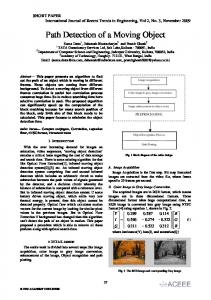
still such a method needs noise removal steps for exact localization of the moving object. Simple image processing tools, like size filters and morphological operators [1][8][12], are proposed after background subtraction and thresholding step. Although they are simple filters, they introduce significant improvement in noise removal and accurate localization. The block diagram of the proposed method is given in Figure 2-1.

Find the Background Image

Figure 2-1

Threshold the Difference Image

Apply Dilation Filtering

Locate the

Apply Size

object

Filtering

Apply Erosion Filtering

Create the Difference Image

Block diagram of IMO detection using background elimination algorithm in stationary camera sequences

Dilation and erosion [1][8] are used consecutively as morphological operators to remove the noise and recover back all the object parts. The pattern of the morphological filters is a 3x3 structure that has a checkerboard pattern as shown in Figure 2-2. This pattern is experimented on thresholded difference images and give satisfactory results.

11

Figure 2-2

The pattern used in dilation and erosion filters

In most cases, there are still some remaining regions after thresholding and morphological operations due to unavoidable noise. Usually, such regions are small and a size filter [1] is used to decrease the false alarm rates due to these noisy regions. In the proposed algorithm, the pixel groups that result in a foreground area that is smaller than 100 pixels are eliminated. The comparative simulation results of this algorithm can be found in Chapter 4.

2.3

Proposed Optical Flow Field-based Method

In this approach, the optical flow field between successive frames is computed and the magnitude field of the motion vectors is thresholded to locate the moving object. A similarity measure filter is added to decrease the false alarm rate. The algorithm is based on the assumption that only the moving objects will create an optical flow field, since the unexpected changes in the scene illumination which may cause optical flow, is minimized due to the small time difference between successive frames. Moreover, the erroneous flow field caused by the camera noise is eliminated by the optical flow estimation itself.

2.3.1 Optical Flow Field Estimation by Pyramidal Kanade Lucas Tracker The most common approach for the analysis of visual motion is based on two phases: Computation of an optical flow field and interpretation of this field [9] The term optical flow field refers both to a velocity field composed of vectors 12

describing the instantaneous velocity of image elements, and a displacement field composed of vectors representing the displacement of image elements from one frame to the next, due to the motion of the camera, the motion of objects in the scene or apparent motion which is a change in the image intensity between frames that mimics object or camera motion. In this section, the computation of the optical flow field and its interpretation to moving object detection in stationary camera sequences are explained. Optical flow field estimation methods are generally based on the minimization of brightness constraint equation [2][13][18][28].

I x ( x , y ) ∗ u ( x , y ) + I y ( x, y ) ∗ v ( x, y ) + I t ( x , y ) = 0

(2-7)

where I x ( x, y ) is the spatial derivative of the image intensity along x-axis, I y ( x, y ) is the spatial derivative of the image intensity along y-axis, I t ( x, y ) is the time derivative of the image intensity between consecutive frames, u ( x, y ) is the horizontal component of the optical flow field and v( x, y ) is the vertical component of the optical flow field. Other constraints, such as smoothness of the neighboring pixels and rigid body motion assumptions [13], are usually introduced to find a solution and also to make the estimation more robust and accurate. Note that the smoothness assumption fails at object boundaries since it is based on the assumption that neighboring pixels will have similar brightness and motion characteristics. There exist algorithms, which try to match some features such as corners, edges, blocks etc. between two or more frames [1][27] to estimate the optical flow. However, the resulting flow field of such algorithms is not dense enough for detection purposes. Apart from these, there are also some methods making use of fitting affine or perspective parameters to motion vectors in a region and estimating the flow field by taking derivatives [13]. The utilized method in this thesis is called Kanade Lucas Tracker [17][18], and it is based on minimization of the brightness constraint equation within a block assuming that the motion vectors remain unchanged over the whole block. The

13

goal of tracking is to find the location of in first image at the second one, such that their intensity differences are minimized, i.e. they are similar. Minimization is achieved within a block to overcome the aperture problem. The resulting optical flow vector is the one which minimizes the constraint function, E (d ) , defined as

E (d ) = E (δx, δy, δt ) =

xi + wx

∑

yi + w y

∑ ( I ( x, y, t ) − I ( x + δx, y + δy, t + δt ))

(2-8)

x = xi − wx y = yi − w y

where I ( x, y, t ) defines the intensity function, ( xi , y i ) defines the point where optical flow estimation is conducted, ( w x , w y ) defines the neighborhood. In this thesis, the minimization is conducted in 5x5 blocks. Accuracy and robustness are two important key points of any tracker [18]. While the accuracy component relates to the local subpixel accuracy attached to tracking, the robustness component relates to sensitivity of tracking with respect to changes of lighting, size of image motion, etc. These two components cannot be introduced at the same time, since one needs small blocksize selection, while the other tends to smooth the images by selecting large block sizes. Hence, there is a natural tradeoff between the robustness and acccuracy components, if one uses traditional methods. In order to overcome this tradeoff, a pyramidal and iterative implementation of the Kanade Lucas Tracker [18][28] is introduced. By applying the pyramidal implementation, the robustness component is satisfied by making the calculations in different resolutions, and the iterative implementation solves the accuracy problem. The pyramidal representation of an image is introduced in a recursive fashion as suggested in [18][28]. The first pyramidal level is the image itself. The second level is computed from the first level by subsampling the first image after applying a lowpass filter to compensate for the anti-aliasing effect [18] ( [1/16 1/4 3/8 1/4 1/16] x [1/16 1/4 3/8 1/4 1/16] is used as the low-pass filter in this implementation). For example, for an image, I, of size 320x240, the consecutive pyramidal image levels I0, I1, I2, I3 are of respective sizes 320x240, 160x120, 80x60 and 40x30.

14

The entire tracking algorithm can be summarized as follows in form of the following pseudo code [18]. Goal : Let p=(x1,y1) be a point on the first image I. Find its corresponding location r=(x2,y2) on the next image J (i.e. J(r,t+δt)=I(p,t) ). I and J are intensity matrices. Build pyramid representations of I and J : {IL}L=0,,Lm {JL}L=0,,Lm

[

g Lm = g xLm

Initialize the pyramidal guess for L = Lm down to 0 with step of

g yLm

] = [0 0] g T

T

-1

Loc. of point p on image IL:

[

p L = px

]

py = p / 2L

L

I L ( x + 1, y ) − I L ( x − 1, y ) I x ( x, y ) = 2

L

I L ( x, y + 1) − I L ( x, y − 1) I y ( x, y ) = 2

Derivative of I wrt x:

Derivative of I wrt y:

Lm

Spatial gradient matrix:

 I x2 ( x, y ) I x ( x, y ) I y ( x , y )  G= ∑   ∑ I y2 ( x, y ) x = p x − wx y = p y − w y    I x ( x, y ) I y ( x, y ) p x + wx

p y + wy

Initialization of iterative tracker:

v 0 = [0 0]

T

for k=1 to K with step of 1 (or until |n| camera is stationary. The algorithm selection procedure directed us to the stationary camera algorithms. At this point, one might use the previously developed approach (background elimination) for IMO detection but since we have the optical flow field, we go on with “the optical flow field approach”. The magnitude field of the optical flow field and its thresholded and morphologically processed version is given in Figure 4-15 . The threshold in this scheme is 0.784. This threshold is computed using mean and standard deviation of the magnitude field, Topt = Mean − 0.2 * Std , as suggested in [15].

58

The statistical parameters, mean and standard deviation, of the resulting vector field are computed for similarity measure calculation. The mean of the motion vectors in x-direction is -7.909 and in y-direction it is 0.0879. The standard deviation of the motion vectors in x-direction is 1.618 and in y-direction it is 0.763. the similarity computed for x and y components are: Similarity of x-component vectors = 0.326 Similarity of y-component vectors = 0.730 Both similarity measures are below the threshold 1. Therefore, the detected objects motion vectors are said to be similar and belong to the same object,

Figure 4-13

Consecutive frames of a sequence taken from a stationary thermal camera

Figure 4-14

A portion of the optical flow field that belong to the IMO

59

(b)

(a)

(c) Figure 4-15

4.4

a) The magnitude field of the optical flow b) Thresholded magnitude field, T=0.784 c) Resulting image after morphological operations

Non-Stationary Camera Results

This section presents the results of IMO detection in non-stationary camera scenes which are mentioned in Chapter 3. Three different schemes for IMO detection in non-stationary camera scenes is presented: Planar scenes, multiplanar scenes and 3D scenes. The results of these different schemes are given separately. The algorithms are applied to artificial and real sequences and the intermediate steps are also presented in order to make more consistent comments on the results. The real data is taken from ‘low resolution thermal camera’ and

60

‘commercial day camera’ sequences and a modified version of the well known ‘flower garden sequence’ is also used during the experiments. The algorithms are applied to the image pairs instead of the whole sequences due to long computation time.

4.4.1 Planar Scene Results Robust recovery of the affine parameters of the dominant plane motion is the most important step in this algorithm. In order to show the accuracy of the affine estimation algorithm, an artificial data is generated by MATLAB. In this data, there exists two planes, which are far away from the camera, but still close to each other. The camera is making translation and rotation. The camera motion parameters are: Tx=0, Ty=0.2, Tz=0.1 ; Ωx=0.05, Ωy=0.05, Ωz=0. The parameters for the first plane are A=18, B=0, C=0, whereas those of the second plane are A=19, B=0, C=0. (Plane equation is Z = A + B X + CY ). The induced and estimated affine parameters of the planes are given in Table 4-1.

Table 4-1

Induced and estimated affines

Plane 1

Plane 2

Estimated Affines

a

-0.05000

-0.05000

-0.054162

b

0.00556

0.00526

0.005411

c

0.00000

0.00000

-0.000048

d

0.06111

0.06053

0.065080

e

0.00000

0.00000

-0.000396

f

0.00556

0.00526

-0.004895

g

-0.05000

-0.05000

-

h

0.05000

0.05000

-

Induced Affine Parameters

61

The algorithm perceived the image as a single plane, since the affine parameters of the planes are very close to each other. The estimated affines are very close to real values , except the 6th parameter, f. Note that, 7th and 8th (g and h) affines are not estimated to make the calculations linear. The results show the effects of linearization on 2D motion field induced by the motion of close planes The detection algorithm is applied to real image pairs taken from a lowresolution thermal camera. At the first step, optical flow field between the image pairs is computed and clustered. Based on the optical flow field characteristics and cluster numbers the camera is identified as non-stationary and the scene is identified as a planar scene. Thus, single 2D parametric registration of the dominant plane process is applied for IMO detection. Figure 4-16 shows two images taken from a rotating thermal camera. The camera is rotating in Y-axis and in clockwise direction. The camera motion is controlled by a two-axis tri-pod.

Figure 4-16

An image pair taken from a moving thermal camera

The integration algorithm is applied to this optical flow field and the result stated that this optical flow field belongs to a non-stationary camera sequence. The related parameters are as follows: Mean of the non-zero motion vectors = 4.585 Magnitude threshold of the motion vectors (0.2 x Mean) = 0.917

62

Number of total pixels = 73040 (332x220) Number of pixels above the threshold = 43248 43248 > %20 of 84480 => camera is non-stationary. Figure 4-17 shows the difference between these two consecutive frames. It is observed that due to the motion of the camera, the difference image is highly cluttered and it is impossible to detect the independently moving car by simple thresholding or by morphological operations.

Figure 4-17

The difference of the image pair given in Figure 4-16

The optical flow field is segmented out and the result is a single plane. The affine parameters of this plane are calculated as follows: a = -4.191942

b = 0.039537

c = -0.161855

d = 0.019666

e = -0.012608

f = 0.015828

Note that the 1st affine parameter dominates the affine parameter space. This is expected, since a = − f c α V x − f c Ω y , meaning that rotation along Y axis directly contributes to 1st affine parameter, a. It is observed that the remaining affine parameters are very small, but still nonzero. This may be due to uncontrolled camera motion (i.e. The camera is not leveled, therefore rotation in Y axis may

63

contribute a small rotation in X axis), measurement noise coming from optical flow field and inherent noise in affine estimation process. Figure 4-18(a) shows the warped state of the second image of Figure 4-17. The warping is achieved according to the estimated affine parameters. Figure 4-18(b) shows the difference between the warped and the first image. It is seen that most of the background is successfully registered. Figure 4-19 shows the thresholded difference image and the result. The threshold is determined as 56 by the Yen algorithm. It is obvious that the result is able to locate the independently moving object.

(a) Figure 4-18

(b) a) Warped second image according to the dominant planes’ affine parameters b) Difference of the warped image and the first image

(a) Figure 4-19

(b)

a) Thresholded difference image, T=56 b) Difference image after morphological operations (erosion and dilation)

64

4.4.2 Multi-Planar Scene Results Reliable clustering of the optical flow field and robust recovery of the affine parameters of each cluster are the most important steps in this scheme, since this method is a modified version of the single parametric registration process. In order to show the accuracy of the clustering and affine estimation algorithms, an artificial data is generated by MATLAB. In this data, there exists three planes, two of them faraway from the camera (planes 2 and 3) but close to each other and the third one (plane 1) close to the camera and two independently moving objects (a truck and a helicopter). Figure 4-20 presents this artificial scene.

3

2

1

Figure 4-20

Artificial scene created at Matlab for ‘MultiLayer Detection Algorithm’ verification

The camera is both translating and rotating. The camera translation creates different 2D image motions for the planes due to their depth difference. The camera motion parameters are selected as: Tx=0 , Ty=0.2 , Tz=0 ; Ωx=0 , Ωy=0.05 , Ωz=0

65

The parameters for the first plane are A=0.5, B=0, C=0, the second planes’ parameters are A=18, B=0, C=0.05 and the third planes parameters are A=18, B=0, C=0.02. (Plane equation is Z = A + B X + CY ) The independently moving objects motion vectors are as follows: Helicopter: u = -0.3 ; v = -0.2

Truck : u = 0.2 ; v = -0.5

The clustering algorithm detected the two planes in the scene and clustered the scene accordingly. The independently moving objects are discarded, since they are small. The third plane is not recognized, since induced motion vectors of 2nd and 3rd planes are very close to each other. Figure 4-21 shows the clustered flow field.

2

1

Figure 4-21

Result of Clustering, white and black indicate two different planes

The induced affine parameters of the planes and the estimated affine parameters are given in Table 4-2.

66

Table 4-2

Induced and estimated affines

Induced Affine Parameters

Estimated Affines

Plane 1

Plane 2

Plane 3

Plane 1

Plane 2

a

-0.05000

-0.05000

-0.05000

-0.051232

-0.054254

b

0.00000

0.00000

0.00000

0.000041

-0.000005

c

0.00000

0.00000

0.00000

-0.000002

-0.000002

d

0.40000

0.01111

0.01053

0.405228

0.012443

e

0.00000

0.00000

0.00021

0.000058

-0.000018

f

0.00000

0.00056

0.00000

-0.000047

0.000026

g

-0.05000

-0.05000

-0.05000

-

-

h

0.00000

0.00000

0.00000

-

-

It is observed that the clustering and affine estimation algorithms are performing quite well and give satisfactory results. Ideally, sequential registration of the planes based on these affines will result for the perfect detection of IMOs. However, in natural sequences clustering of the optical flow field is not perfect, since the estimated optical flow field contains some errors. The exact boundaries of the planes are difficult to detect; in fact the planes may even not have exact boundaries. In addition, the optical flow field is not fully dense. These reasons cause errors in clustering and affine estimation. This fact is illustrated in a typical image sequence. Figure 4-22 shows two consecutive frames taken from the “Flower Garden Sequence”, where the camera is translating to the right. Figure 4-23 shows a down-sampled version of the optical flow field between these consecutive frames. Down sampling is achieved just for illustrative purposes. The planes at different depths have different motion vectors, since the camera is performing translational motion. Figure 4-24 shows the segmented optical flow field. The tree, the flower garden and the sky is segmented almost properly. The improperly segmented parts are due to noise coming from optical flow field calculation, the optimization of the inner parameters of segmentation process.

67

Figure 4-22

Two consecutive frames from “Flower Garden Sequence”

Figure 4-23

Optical Flow Field between the frames given in Figure 4-22

68

Figure 4-24

Result of segmentation. Number of segments is 5.

The same segmentation framework is applied to a multilayer scene for IMO detection. Figure 4-25 shows two consecutive frames taken from a day camera. The camera is translating to the right.

Figure 4-25

Two consecutive frames taken from a day camera

69

Figure 4-26

a) Optical Flow between the frames b) Segmented optical flow field. Number of segments is 3

Figure 4-26 shows the resulting estimated optical flow field between these frames and the result of the segmentation for the optical flow field. The number of segments is determined as 4. Some flow vectors are not processed since none of the affines is able to fit within acceptable error limits. For example, most of the flow vectors belonging to the tree branch at the top right are not processed. The zero and non-reliable flow vectors are painted to white in the resulting segmentation image. The helicopter is not segmented out since it is small. The reliable segments are used in consecutive registration for IMO detection. The affine parameters of these planes are given in Table 4-3.

Table 4-3

Affine parameters of the segments (planes)

Estimated Affine Parameters Plane 1 (foreground)

Plane 2 (background)

Plane 3 (mast)

a

2.990174

0.697773

9.287494

b

-0.000058

-0.009532

0.002393

c

0.044135

-0.001776

0.007251

d

0.053848

0.019301

-0.467732

e

-0.001887

-0.001620

0.000595

f

0.001606

-0.000248

0.006704

70

The difference in the motion characteristics of the planes can easily be observed from the affine parameters. The mast (i.e. the electricity beam) that is very close to the camera has the highest affine parameter set. The foreground and background layers have smaller affine parameters, respectively. The registration starts with the largest plane and continues with the preceding large plane. Figure 4-27 shows the original difference image, the difference after warping the mast as an intermediate step, and the result of the registration process followed by thresholding and morphology.

(b)

(a)

Figure 4-27

a) The difference image between the frames of Figure 4-25 b) The difference image after the warping of the mast

(a)

Figure 4-28

(b)

a) The final thresholded difference image after all the planes are warped. b) The result after morphological operations are applied

71

4.4.3 3D Scene Results 2D parametric registration of the dominant plane and parallax rigidity constraint utilization enable the detection of independently moving objects in the scenes which have dense or sparse parallax motion. In order to show the accuracy of the parallax rigidity constraint algorithm, an artificial data is generated by MATLAB. In this data, there exists 8 planes at different depths and with different surface parameters, since this must be a 3D scene. In addition, there exist two IMOs in the same scene. Application of the parallax rigidity constraint requires three consecutive frames, therefore the camera makes two sets of motions to generate the artificial optical flow fields. The camera is making translation and rotation both. The camera motion parameters are Motion 1 : Tx1 = 0 , Ty1 = 0.2 , Tz1 = 1.5 ; Ωx1 = 0.25 , Ωy1 = 1.5 , Ωz1 = 0 Motion 2 : Tx2 = 0 , Ty2 = 0.2 , Tz2 = 1.5 ; Ωx2 = 0.25 , Ωy2 = 1.5 , Ωz2 = 0 The motion parameters of the independently moving objects are: Helicopter:

u1 = -1.1 ; v1 = -0.2

u2 = -1.1 ; v2 = -0.2

Truck :

u1 = -2 ; v1 = -0.5

u2 = -2 ; v2 = -0.5

For generating the artificial data, the optical flow vectors u and v is computed at every image point using the plane parameters, and camera motion parameters as derived in Chapter 3. The affine parameters for each plane is computed by using the formulas

u = a + b x + c y + g x 2 + h xy , v = d + e x + f y + g xy + h y 2 Figure 4-29 shows the 3D scene generated by MATLAB.

72

7

6 8

4

3 2

5

Figure 4-29

1

3D scene generated by MATLAB

The plane parameters are given in Table 4-4.

Table 4-4

The plane parameters of the 3D scene

A

B

C

Plane 1

0.8

0

0

Plane 2

1.2

0

0

Plane 3

2

0

0

Plane 4

2.5

0

0

Plane 5

2

0.03

0.05

Plane 6

7

0

0

Plane 7

8

0

0

Plane 8

158

0

0

In order to apply the parallax rigidity constraint to this sequence, one of the planes should be parametrically aligned to remove the effects of rotation. Figure 4-30 shows the result of parallax rigidity constraint applied for IMO detection when the 2D parametric registration step skipped. This result is presented to show the effect of registration process. 73

Figure 4-30

Parallax rigidity constraint applied to the artificial data without 2D parametric registration.

The reference point is located at bottom of plane 4. This is a proper choice since it belongs to the static background. The helicopter is detected because moves in the opposite direction. However, the truck cannot be detected, since it does not have an extreme motion characteristic. In addition, plane 3 and plane 4 seem to violate the parallax rigidity constraint. When one registers one of the planes and apply rigidity constraint, the results become much more reliable as shown in Figure 4-31.

Figure 4-31

Parallax rigidity constraint applied to the artificial data after 2D parametric registration

74

The registration is conducted according to the parameters of plane 6 (mountain). The same point on plane 4 is selected as reference. Figure 4-31 implies that the parametric registration removes all the effects of rotation and the rigidity constraint can be perfectly applied. The static background is totally eliminated with this algorithm, although different planes belonging to the static background have different 2D image motions. The same algorithm is applied to a three-frame sequence taken from a day camera. The algorithm makes the reference point selection and plane registration automatically. Figure 4-32 shows these 3 frames. The reference point is selected using the Harris corner detector. Figure 4-33 shows the corner map of the first image. The highest density corner is on top of the right hand-side tree as marked. In this sequence camera only makes Z-translational motion. Therefore, the 2D parametric registration process is useless and is not conducted. Figure 4-34(a) shows the difference image of the first two frames. It is observed that moving objects cannot be identified from the difference image. Figure 4-34(b) shows the parallax rigidity constraint applied to this scenario. The algorithm reliably detected the independently moving objects (cars), since they are violating the rigidity constraint.

75

Figure 4-32

Three consecutive frames taken from a translating camera

Figure 4-33

Corner map of the first frame of Figure 4-32. The highest density corner point is at the middle of the circle.

76

(b)

(a)

Figure 4-34

a) The difference image of the first and second frame.. b) The result of parallax rigidity constraint without 2D parametric registration

In order to show the effect of registration, the algorithm is applied to a sequence where the camera is performing both translation and rotation. The sequence is again taken from a day camera. Figure 4-35 shows three frames taken from this sequence.

Figure 4-35

Three consecutive frames taken from a rotating-translating day camera

77

The optical flow field between these frames is segmented out and 7 different planes are detected. Figure 4-36 shows the result of segmentation. The largest segment (plane) is registered for parallax rigidity constraint application. The reference point is determined on top of the background plane composed of trees as marked in the first image.

Registration plane

Figure 4-36

Result of segmentation. Number of segments is 7.

Figure 4-37

a) Result of Parallax Rigidity before registration b) Result of Parallax Rigidity after registration

78

Figure 4-37 shows results of “Parallax Rigidity Constraint” applied to the sequence before and after registration. The registration process removed the effect of camera rotation and the result became more visible.

79

CHAPTER 5 CONCLUSIONS AND FUTURE WORK

Automatic independently moving object detection is an important goal in video surveillance applications, for guidance of autonomous vehicles, for efficient video compression, for smart tracking, for automatic target recognition (ATR) systems, for terminal phase missile guidance, and for many other applications. In this thesis, independently moving object detection problem is analyzed for different camera motions and scene structures. The detection methodology may vary for different applications. However, the solution for one case can be a preprocessing step for the others. At the first glance, the problem should be separated into two classes: Moving Object Detection in Stationary Camera Sequences and in Non-Stationary Camera Sequences and examined separately. In stationary camera sequences, two solutions were proposed: Background Elimination and Optical Flow Based Method. The background elimination method gives promising results in the controlled environments, when the camera is strictly fixed. The reliability of the background extraction process turns out to be the most important step in this method. The best results can be obtained, when “moving average selectivity method” is used for background extraction. Thresholding and morphological operations steps are also very important for binarization and localization of the detection results. Yen’s method based on histogram entropy is utilized for automatic threshold selection. The experiments show that adaptive selection of the threshold for each image pair gives more promising results than a global threshold selection. The simulations also show that the morphological operations, erosion and dilation, improve results in object localization, although they are very simple. An important property of the tested method beside its

80

reliability, is its simplicity and low computational cost. In a controlled environment, the method can be used for moving object detection even with low-cost hardware. The second method for moving object detection for stationary camera sequences makes use of the optical flow field induced between consecutive frames. Ideally, the optical flow field and the motion field are identical. The optical flow field is determined by a hierarchical version of Kanade Lucas Feature Tracker. The optical flow computation is applied to various kind of frames containing day camera frames, thermal camera frames and artificial frames and the results are quite satisfactory. In stationary camera sequences, the non-zero optical flow field points the moving object, since ideally the static background will not cause any change in scene intensity character. The experiments show that, the magnitude of the optical flow field between two consecutive frames taken from a stationary camera can be used for moving object detection after simple thresholding and morphological operations. The results of this detection scheme are reliable and satisfactory while the computation time is quite high compared to background elimination method. Therefore, using this method in stationary camera sequences can be seen unreasonable at the first glance. However, the optical flow computation is the base step for moving object detection in non-stationary camera sequences as well. Moreover, if the detection is conducted in an uncontrolled environment, where the camera makes various kinds of motions and the scene structure changes frequently within the sequence, the optical flow field should be calculated in any case. This calculation is also necessary for post-processing steps and for model discrimination. Therefore, using the optical flow field for stationary camera sequences should be a part of the algorithm integration process. In non-stationary camera sequences, different algorithms are proposed for different camera motion characteristics and scene structures. For rotating cameras and/or planar scenes, 2D parametric registration of the dominant plane is used for moving object detection. Segmentation of the optical flow field is introduced in this step to distinguish between the multi-layer and single layer scenes. An affine parameters based method was used for optical flow field segmentation. The experiments on artificial and real data indicate that the affine parameter estimation is reliable, if the scene can be segmented properly. Proper segmentation is achieved if the internal parameters of the algorithm are optimized. It is observed

81

that this optimized values vary for different scenes, therefore, it is difficult to find global parameters for these values. However, manual optimization gives satisfactory results in moving object detection framework. In the planar scenes, segmentation process generally results in single planar motion, thus the registration is conducted with the affine parameters of this plane. The experiments indicate that 2D parametric registration is enough for most of the planar scenes to detect moving objects, and for all rotating-only camera scenes. A modified version of the 2D parametric registration process is used for multi planar scenes. When the scene cannot be modeled by a single plane and the camera makes translational motion, the 2D parametric registration of the dominant plane is not sufficient. In this kind of scenes, the segmentation process results in two or three planes. Moving object detection is achieved by sequential registration of these planes. However, if the moving object is large, then it can also be detected as a plane. This scenario is not tested but some methods are proposed in the literature to solve this case. When the depth variation within the scene is high and the scene cannot be modeled by layers, a parallax based approach is proposed for moving object detection. This method is based on the observation that when camera makes translational motion, the planes at different depths induce different 2D motions according to their depth and plane parameters. In addition, the static background move in an organized fashion, named parallax rigidity. The independently moving objects do not obey this parallax rigidity rule; therefore, parallax rigidity constraint is used for independently moving object detection. Before applying parallax rigidity, 2D parametric registration is required to remove the effects of rotation and create a translation-based framework. The experiments on artificial and real data show that the algorithm gives satisfactory results, when 2D registration is properly applied. Moreover, this parallax-based approach is also experimented in sequences where the parallax information is sparse with respect to the independent motion, and the results are still satisfactory. This property makes this algorithm more reliable compared to the classical plane+parallax based approaches where the epipole is used for independent motion detection. The reference point and registration plane selection is achieved automatically, as a difference from the literature.

82

In real image sequences it is possible to face with stationary, nonstationary, rotating-only, translating-only, rotating and translating cameras and planar, multi-planar and dense depth scenes. Therefore, none of the algorithms can be applied to the whole sequence. In order to make the detection problem more useful and applicable, an integration of the algorithms is strictly required. An optical flow and segmentation based unification is proposed in this thesis. The density and variance of the optical flow field is used to discriminate two cases: stationary camera and non-stationary camera. The statement is based on the fact that if the camera is not moving the optical flow field will be zero everywhere other than the moving object areas and if the camera is moving the optical flow field will be non-zero almost at every point. The experiments on real sequences indicate that this is a reliable reasoning and can be used for stationary/non-stationary discrimination. On the other hand, the model discrimination within non-stationary camera sequences is more complex. The optical flow field is segmented into regions and the number of reliable segments give valuable information about the scene and camera motion structure. If the number of reliable segments is 1, then 2D parametric registration approach will be sufficient for moving object detection. If the number of segments is between 2 and 4, then the scene is modeled by plane patches and sequential registration is applied. Finally, if the number of segments is greater than 4, parallax rigidity based approach is applied. This procedure is experimented with real sequences with a limited data set and gave satisfactory results. However, the segmentation process is very critical in this approach and it may require manual interaction for optimization. Therefore, more consistent unification approaches, which include temporal analysis, is required and is left as a future work. The implicit usage of the ego-motion (camera motion) parameters in IMO detection gives us valuable information about navigation characteristics (3D velocity/acceleration and rotation angles) of the platform, where the camera is mounted. Therefore, the approaches mentioned in this thesis can be integrated to commonly-used navigation systems. For example, the integration of this work to ‘Inertial Navigation Systems’. via Kalman Filter, named ‘Image Aided Inertial Navigation via Kalman Filtering’ [29], will be an attractive issue to work on. This integration will be useful for autonomous navigation of mobile robots, long-term

83

navigation and terminal guidance of cruise missiles, sight lining of helicopter or other moving-platform weapon systems. Moreover, the parallax based approach is considered to be an attractive framework for 3D reconstruction and scene analysis.

84

REFERENCES

[1]

Jain, R. , Kasturi, R. , G.Schunk, B. , “Machine Vision”, McGRAW-HILL

International Editions, 1995.

[2]

Klaus, B. , Horn, P. , “Robot Vision”, MIT Press, 1986

[3]

Tzannes, A.P. , Brooks, D.H. , “Point Target Detection in IR Image

Sequence: A Hypothesis-Testing Approach Based on Target and Clutter Temporal Profile Modeling”, Opt. Eng., Vol 39, No. 8, pp. 2270-2278, August 2000

[4]

Soni, T. , Zeidler, J.R. , Walter, H.K. , “Detection of Point Objects in

Spatially Correlated Clutter Using Two Dimensional Adaptive Prediction Filtering”, http://citeseer.ist.psu.edu/21704.html, 1992

[5]

Rosin, P.L. , Ellis, T. , “Image Difference Threshold Strategies and Shadow

Detection”, British Machine Vision Conf., pp. 347-356, 1995

[6]

Irani, M. , Anandan, P. , “A Unified Approach to Moving Object Detection in

2D and 3D Scenes”, IEEE Transactions on Pattern Analysis and Machine Intelligence, Vol. 20, No. 6, June 1998

[7]

Irani, M. , Rousso, B. , Peleg, S. , “Robust Recovery of Egomotion” , Proc.

of CAIP, pp. 371-378, 1993

[8]

Strehl, A. , Aggarwal, J.K. , “MODEEP: a motion-based object detection and

pose estimation method for airborne FLIR sequences”, Machine Vision and Applications, Springer-Verlag, 2000

85

[9]

Adiv, G. , “Determining three-dimensional motion and structure from optical

flow generated by several moving objects”, IEEE Transactions on Pattern Analysis and Machine Intelligence, VOL. PAMI-7, No. 4, July 1985

[10]

Piccardi, M. , “Background Subtraction Techniques: a review”, University of

Technology Sydney, 2004

[11]

Stauffer, C. , Grimson, W.E.L. , “Adaptive Background Mixture Models for

Real-Time Tracking”, Proc. Of CVPR, pp. 246-252, 1999

[12]

Borghys, D. , Verlinde, P., Perneel, C. , Acheroy, M. , “Multi-level Data

Fusion for the Detection of Targets using Multi-Spectral Image Sequences”, Opt. Eng., Vol. 37, No. 2, pp. 477-484, February 1998

[13]

Alatan,

A.

,

“Lecture

Notes

of

Robot

Vision

Class,

EE701”,

Electrical&Electronics Engineering Department, METU, 2002

[14]

Malvika, R. , “Motion Analysis, Course notes for CS558”, School of

Computer Science, McGill University

[15]

Sankur, B. , Sezgin, M. , “A survey over Image Thresholding Techniques

and Quantitative Performance Evaluation”, Journal of Electronic Imaging, Vol. 13, pp. 146-165, January 2004

[16]

Kapur, J.N. , Sahoo, P.K. , Wong, A.K.C. , “A new method for Gray-Level

Picture Thresholding Using the Entropy of the Histogram”, Computer Vision, Graphics and Image Processing 29, 273-285, 1985

[17]

Lucas, B. , Kanade, T. , “An iterative image registration technique with an

application to stereo vision”, Proc. Image Understanding Workshop, 1981

86

[18]

Bouget, J.Y. , “Pyramidal Implementation of the Lucas Kanade Feature

Tracker, Description of the Algorithm”, Intel Corporation, 1999

[19]

Irani, M. , Rousso, B. , Peleg,S. , “Computing Occluding and Transparent

Motions”, Int’l J. of Computer Vision, Vol. 12, p. 5-16, Feb 1994

[20]

Wang, J.Y.A. , Adelson, E.H. , “Representing Moving Images with Layers”,

IEEE Transactions on Image Processing Special Issue: Image Sequence Compression, Vol. 3, No. 5, p. 625-638, September 1994

[21]

Lourakis, M.I.A. , Argyros, A.A., Orphanoudakis, S.C. , “Independent 3D

Motion Detection Using Residual Parallax Normal Flow Fields”, ICCV, pp. 10121017, 1998

[22]

Ben-Ezra, M. , Peleg, S. , Rousso, B. , “Motion Segmentation Using

Convergence Properties”, ARPA Image Understanding Workshop, November 1994

[23]

Irani, M. , Rousso, B. , Peleg, S. , “Recovery of Ego-Motion Using Region

Alignment”, IEEE Transactions on Pattern Analysis and Machine Intelligence, Vol. 19, No. 3, p. 268-272, March 1997

[24]

Irani, M. , Anandan, P. , Cohen, M. , “Direct Recovery of Planar-Parallax

from Multiple Frames”, IEEE Transactions on Pattern Analysis and Machine Intelligence, Vol. 24, No. 11, November 2002

[25]

Harris, C., Stephens, M. , “A combined Corner and Edge Detector”, Plesey

Research Roke Manor, UK, The Plessey Coompany plc. , 1988

[26]

Borshukov, G.D. , Bozdagi, G. , Altunbasak, Y. , Tekalp, M. , “Motion

Segmentation by Multistage Affine Classification”, IEEE Transactions on Image Processing, Vol. 6, No. 11, November 1997

87

[27]

Qian, G. , Chellappa, R. , “Moving Targets Detection using Sequential

Importance Sampling”, Proc. of Int’l Conf. on Computer Vision, Vol 2, pp. 614-621, July 2001

[28]

Irani,

M.

,

Anandan,

P.

,

“All

About

Direct

Methods”,

Vision

Algorithms:Theory&Practice, Springer-Verlag, 1999

[29]

Giebner, M. G. , “Tightly-Coupled Image-Aided Inertial Navigation System

via a Kalman Filter”, AIR FORCE Inst. Of Tech. Wright-Patterson School of Enginerring and Management, Master’s Thesis, March 2003

[30]

Duda, R.O. , Hart, P.E. , “Pattern Classification and Scene Analysis”, John

Wiley, 1973

[31]

http://mmrg.eee.metu.edu.tr/imageutil http://mmrg.eee.metu.edu.tr/videoutil

88