I. INTRODUCTION
Moving Targets Processing in SAR Spatial Domain
PAULO A. C. MARQUES, Member, IEEE Instituto Superior de Engenharia de Lisboa Portugal ´ M. BIOUCAS DIAS, Member, IEEE JOSE Instituto de Telecomunica¸co˜ es Portugal
This paper presents a novel technique to estimate the initial coordinates and velocity vector of moving targets, including those with velocities above the Nyquist limit, using a single synthetic aperture radar (SAR) sensor without increasing the pulse repetition frequency (PRF). The basic reasoning is that, although the returned echoes may be undersampled in the azimuth direction, their phase and amplitude are informative with respect to the moving target trajectory parameters. Therefore, the so-called blind angle ambiguity, inherent to systems using a single SAR sensor, is overcome. The proposed method samples the data in the spatial domain, along the signature curve which depends on the moving target trajectory parameters. The resulting algorithm is a highly efficient (from the computational point of view) 1D matched filter. The effectiveness of the proposed scheme is illustrated using simulated SAR data and real data from the MSTAR public release data set, corresponding to a static SAR scene and a static BTR-60 with simulated motion.
Manuscript received January 30, 2005; revised April 24, 2006; released for publication October 18, 2006. IEEE Log No. T-AES/43/3/908396. Refereeing of this contribution was handled by D. J. Salmond. This work was supported by Projects PDCTE/CPS/49967/2003 and IPL-5828/2004. Authors’ addresses: P. Marques, Instituto Superior de Engenharia de Lisboa and the Instituto de Telecomunica¸co˜ es, R. Conselheiro Emidio Navarro 1, 1959-007 Lisbon, Portugal, E-mail: (
[email protected]); J. Dias, Instituto de Telecomunica¸co˜ es and the Instituto Superior Te´ cnico, Av. Rovisco Pais 1, 1949-001 Lisbon, Portugal.
c 2007 IEEE 0018-9251/07/$25.00 ° 864
The synthetic aperture radar (SAR) community is presently researching, among other topics, the detection and imaging of moving targets for surveillance purposes. Many applications aim at determining the position and the velocity of moving targets. The purpose may be, for example, to find traffic jams [1] or to detect ships in the sea [2]. Other civil applications include oil pollution monitoring and surface currents measurement [3]. Some military applications are also oriented towards detecting and recognizing moving targets [4]. The purpose may be to intercept targets threatening facilities or resources. In other scenarios the purpose may be to keep the moving objects safely apart from each other as they navigate, thus requiring accurate detection, high resolution imaging, and precise kinematics estimation. This paper, which elaborates on ideas presented in [5], addresses the design of a processing scheme aiming at trajectory estimation of multiple moving objects in SAR, using a single sensor. When the data is acquired using a single SAR sensor, it is generally accepted that: 1) the azimuth position uncertainty (also termed blindangle ambiguity) cannot be solved [6, ch. 6], [7], and 2) the maximum unambiguous moving target velocity is bounded by the Nyquist velocity imposed by the pulse repetition frequency (PRF) [7, 8]. Recently, the authors have shown in [9], [10], and [11] that a proper processing of the phase and amplitude of the received signal overcomes the aforementioned limitations. In [10], we have already presented an accurate method to detect and to estimate the initial coordinates and velocity vector (assuming no acceleration and no rotational motion) of moving targets using a single SAR sensor. Herein, we present a novel technique much lighter from the computational point of view, although less accurate, to estimate the initial coordinates and velocity vector of a moving target using data from a single SAR sensor. In fact, the primarily aim of the work presented here is moving target trajectory estimation and not moving target detection. Several methods are published in the recent literature to efficiently deal with the detection problem such as [12]. Nevertheless, we herein adopt a simple technique that works reasonably well, namely, for illustration purposes. The detection and estimation scheme proposed in [10] uses a matched filtering operation, depending on the moving target parameters, that simultaneously copes with range migration and compresses two-dimensional signatures into one-dimensional ones without degrading the slant-range resolution. The resulting methodology simultaneously detects moving targets and estimate their motion parameters. We focus here mainly on the estimation side of the problem, presenting a more efficient technique, from the computational point of view, when compared
IEEE TRANSACTIONS ON AEROSPACE AND ELECTRONIC SYSTEMS VOL. 43, NO. 3
JULY 2007
with the estimation procedure presented in [10]. The algorithm samples the spatial domain and, in contrast with the previous approach, the moving target signature is not straightened. Instead, it processes data along the signature curve that depends on the moving target trajectory parameters. To keep the computational requirements low in the global scheme, the estimation algorithm is guided by a simple moving target detection algorithm as referred above. Therefore, the estimation algorithm only processes data belonging to confined regions of the target area. The detection of the moving targets consists in first applying a high-pass filter in the 2D frequency domain with stop-band adjusted to filter out static targets, and then performing imaging using static ground parameters. The resulting image displays the defocused and misplaced moving targets images, even if their slant-range velocity is a multiple of the Nyquist velocity, as far as their respective 2D spectrum exhibits a nonnegligible skew. The estimation algorithm uses both the phase and the amplitude information of each moving target signature and is able to retrieve all the moving target trajectory parameters using a single SAR sensor. The obtained accuracy is high, provided that the clutter spectra does not overlap completely that of the target. Otherwise, the results are meaningful only if the signal-to-clutter ratio (SCR) is higher than 10 dB. The paper is organized as follows. In Section II we write the received signal, after pulse compression, in the spatial domain, parameterized by the trajectory parameters. By assuming that the moving target signature is immersed in white noise, we derive a maximum likelihood (ML) estimator for the moving target trajectory parameters. In Section III, the proposed moving target trajectory estimation algorithm is described and its computational complexity is analyzed. In Section IV, we present results using simulated SAR data and real data from the MSTAR public release data set, corresponding to a static SAR scene and a static BTR-60 with simulated motion.
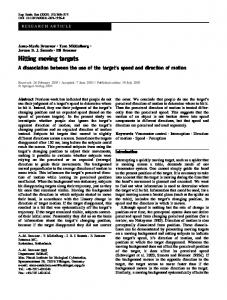
Fig. 1. SAR slant-plane. At cross-range position u0 , radar is broadside to moving target.
target, after quadrature demodulation and pulse compression, is given by s(x, u) ´ a(y0 ¡ ºu)pc [x ¡ r(u)]fm e¡j2k0 r(u)
(1)
where x = ct=2, a(¢) is the two-way antenna radiation pattern, º ´ 1 + b, pc (x) is the compressed transmitted pulse in the slant-range direction, fm is the moving target complex reflectivity, k0 ´ 2¼=¸0 is the wavenumber at wavelength ¸0 , and r(u) is the distance between the platform and the moving target, given by q r(u) ´ (x0 ¡ ¹u)2 + (y0 ¡ ºu)2 : (2) It is assumed that a(u) does not depend2 on x, and that there are no pointing errors of the antenna. Let us define u0 ´ u ¡ u0 such that u0 = 0 corresponds to the position of the radar when the moving target is broadside to it. Therefore, defining r0 (u0 ) ´ r(u0 + u0 ) and noting that y0 ¡ ºu0 = 0, we obtain p r0 (u0 ) = (x0 ¡ ¹u0 )2 + (¡ºu0 )2 : (3) Approximating r0 (u0 ) by a series expansion about u0 = 0 and retaining only the terms through the quadratic, results º2 r0 (u0 ) ¼ x0 ¡¹u0 + 0 u02 | {z2x }
(4)
Ã(u0 )
II. ESTIMATION SCENARIO Fig. 1 illustrates a moving target with slant-range and cross-range coordinates (x0 , y0 ), when the platform is at position u = 0, and velocity (vx , vy ) = (¹vR , bvR ) defined in the slant-plane (x, y); symbol vR denotes the platform speed and (¹, b) is the target relative velocity with respect to the radar.1 Let us define (x0 ´ x0 ¡ ¹u0 , y 0 ´ u0 ) as the moving target coordinates when the radar platform is broadside to the target. When the radar is positioned at coordinate y = u, the corresponding received echo from a moving 1 Velocities
vx and vy are directed opposite to x and y.
valid for ju0 j ¿ x0 . Assume that the range migration Ã(u0 ) is known. We can then acquire data along coordinates s0 (x, u0 ) ´ s[x = x0 + Ã(u0 ), u0 + u0 ], leading to 0 0 s0 (x, u0 ) = a(¡ºu0 )pc (0)fm e¡j2k0 r (u ) : (5) Since pc (³) exhibits high resolution about ³ = 0, then s0 (x, u0 ) becomes clustered about x = x0 + Ã(u0 ), for all u0 in the support of a(¢). Therefore, we can form a vector containing the signature samples echoed by the moving target. 2 As shown in [10, eq. (21)], the range dependence of the antenna pattern can be neglected if the length of the swath is much smaller than the coordinate of the swath center.
MARQUES & DIAS: MOVING TARGETS PROCESSING IN SAR SPATIAL DOMAIN
865
Let us assume that pc (0) = 1 and that the clutter is white in the spatial domain [13]. Let z(x, u0 ) = s0 (x, u0 ) + n(x, u0 ) be the signal plus noise, respectively. Define vectors z ´ [z¡N , : : : , z0 , : : : , zN ]T s ´ [s¡N , : : : , s0 , : : : , sN ]
Parameters u0 , x0 , and y0 are then computed as follows: uˆ 0 = u0 + ˆi0 us
T
where, for i = ¡N, : : : , N, zi = z[x0 + Ã(u0i ), u0i ] 0
0
si = a(¡ºu0i )e¡j2k0 r (ui ) with u0i ´ u0s i, where u0s is the sampling space in the cross-range direction chosen such that the clutter samples exhibit negligible correlation. In fact, if we assume homogeneous clutter, then the autocorrelation of the signal echoed by the ground is Rn (¢u) / F ¡1 [jA(ku )j2 ] as shown in [13], where F ¡1 stands for the inverse Fourier transform and A(ku ) is the antenna radiation pattern in the slow-time frequency domain. If the bandwidth of jA(ku )j is B, then the correlation Rn (¢u) is approximately zero for ¢u = vR =B. The samples are therefore uncorrelated if taken with spacing of ¢u = vR =B. The observation vector z should be formed with data sampled along the curve described by Ã. However, in practical situations, SAR raw-data is available only at discrete values of (x, u0 ). For a fixed u0i , the corresponding slant-range coordinate is x0 + Ã(u0i ), and, in general, this coordinate does not correspond to a multiple of the sampling space in the slant-range direction. Therefore, a resampling or data interpolation should be done in the slant-range dimension. Nevertheless, as illustrated in Section IV, a simple nearest neighbor interpolation method may lead to satisfactory results. Let us assume that the moving target parameters μ ´ (¹, º, x0 , y 0 , u0 ) and the reflectivity fm are known. In this case only the noise term is random. Therefore, the density of vector z conditioned to μ and fm is p(z j fm , μ) » N (¹z , Cz )
(6)
where the mean is ¹z ´ fm s(μ), the covariance is Cz ´ ¾n2 I, and the clutter variance is ¾n2 . Notice that zi = zi (μ). Consequently, the density in (6) is correct only for the true μ. However, for μ ' μ0 , the range migration is known and the data taken to form vector s is acquired along the correct curve, thus leading to z(μ) ' z(μ0 ). Therefore, we still use (6) to compute the ML estimate of μ. After some algebra, we obtain P ¤ j z s (μ)j (7) μˆ ML = arg max P i i i 2 : μ js i i (μ)j We note that u0 is not exactly known. However, assuming that u0 is a multiple of us , i.e., u0 = us is , then an error on u0 corresponds to an integer shift i0 866
on the sequence zi . For this reason, we replace the numerator of (7) by a correlation, obtaining P ¤ ½ ¾ j i zi si¡i (μ)j 0 ˆ ˆ º, ˆ i0 )ML = arg max max P (¹, : (8) 2 i0 (¹,º) i jsi (μ)j
(9)
xˆ 0 = x0 + ¹ˆ uˆ 0
(10)
yˆ 0 = (ºˆ ¡ 1)uˆ 0 :
(11)
Notice that, by using the methodology herein presented, we are able to estimate not only the full velocity vector (¹, º), but also the initial coordinates (x0 , y0 ) of the moving target, thus solving the blind angle ambiguity. III. MOVING TARGET PARAMETER ESTIMATION ALGORITHM Algorithm 1 presents pseudocode for the procedure entitled ProcessMultipleTargets, which aims at the detection and trajectory parameter estimation of multiple moving targets. It starts by searching for all the moving targets in the target area, using function SearchStrongestTargets. Then, for each moving target, the algorithm increases the SCR by digitally spotlighting the moving target area [14]. This process consists of focusing the target area with static ground parameters (recall that the true moving target parameters are unknown) and cropping the region containing the target of interest. Although the moving targets will appear defocused, they span a region that is typically much smaller than the total illuminated scene. Each moving target signature can thus be reasonably separated from the signatures of the other (moving and stationary) targets. The algorithm then resynthesizes the signature of the digitally spotlighted object to the (x, u) spatial domain, via reversing the wavefront reconstruction algorithm steps (see [10] for a brief description of the wavefront algorithm). Function GetParameters, which is described in Algorithm 3, is then used to estimate parameters (x0 , u0 , ¹, º) of each detected moving target. Algorithm 2 describes function SearchStrongestTargets which implements a very simple but efficient scheme (from the computational point of view), to detect all the moving targets in the target area. It takes as input S(!, ku ) = F(t,u) [s(t, u)], i.e., the 2D Fourier transform of s(t, u) and returns Xc , Yc , Nt , and s(X, Y), where Xc , Yc is the array with the estimated positions of the all the detected moving targets, Nt is the number of detected targets, and s(X, Y) is the target area focused with static ground parameters. It should be stressed that the goal here is to present and evaluate a strategy for moving target trajectory parameters estimation and as such
IEEE TRANSACTIONS ON AEROSPACE AND ELECTRONIC SYSTEMS VOL. 43, NO. 3
JULY 2007
ALGORITHM 1 ProcessMultipleTargets 1: [Xc , Yc , Nt , s(X, Y)] := SearchStrongestTargets[S(!, ku )] 2: for i := 1 : Nt do 3: sˆ(x, u) := InverseWaveFront[s(X, Y) ¤ MASK(Xc (i), Yc (i))] ˆ º(i)) ˆ 4: (xˆ 0 (i), yˆ 0 (i), ¹(i), := GetParameters[sˆ(x, u)] 5: end for ALGORITHM 2 Function [Xc , Yc , Nt , s(X, Y)] := SearchStrongestTargets[S(!, ku )] Initialization: ´, Nt = 0, HHPF (!, ku ) := HighPassFilter 1: SF (!, ku ) := S(!, ku )HHPF (!, ku ) fremove static objectsg 2: sF (X, Y) := WaveFront[SF (!, ku ), ® = 1] ffocus moving targets with static ground parametersg 3: repeat ˆ Y, ˆ l) := GetMaxPos[abs(s (X, Y))] 4: (X, F fget position and value of strongest pixelg 5: if l >= ´ then 6: Nt := Nt + 1 ffound another candidateg ˆ Y (N ) := Yˆ fstore its coordinatesg 7: Xc (Nt ) := X, c t ˆ Y) ˆ fand remove itg 8: s (X, Y) := s (X, Y)MASK(X, F
F
9: end if 10: until l < ´ 11: s(X, Y) := WaveFront[S(!, ku ), ® = 1] fand return the data focused with static ground parametersg
ˆ º) ˆ := GetParameters[sˆ (x, u)] ALGORITHM 3 Function (xˆ 0 , yˆ 0 , ¹, M¹ º , fºi gM Initialization: f¹i gi=1 i=1 1: (xˆ 0 , u0 ) := GetSignatureCenter[sˆ(x, u)] 2: u0 := u ¡ u0 3: for i := 1 : M¹ do 4: for j := 1 : Mº do 5: z := s(xˆ 0 + Ã(u0 ), u0 ) fform vector using data extracted along curve given by expression (4) 6: o := Correlation(z, s) fcorrelation (8)g 7: [value, coord] := GetMax(o) 8: if value > max then [found higher objective function value] 9: max := value 10: i0 := coord 11: ¹ˆ := ¹(i) 12: ºˆ := º(j) 13: end if 14: end for 15: end for 16: uˆ 0 := u0 + i0 us 17: yˆ 0 := (ºˆ ¡ 1)uˆ 0 18: xˆ 0 := xˆ 0 + ¹ˆ uˆ 0 it uses, for illustration purposes only, a very simple methodology for moving target detection. Other efficient techniques are published in the literature such as [12]. The scheme implemented by function SearchStrongestTargets is now summarized. The returns from the static ground in the 2D frequency domain are filtered and compressed using the wavefront reconstruction algorithm with static ground parameters (® = 1). The signal that remains after filtering and focusing corresponds to the returns from moving targets with velocities inducing Doppler-shifts and/or scalings on the returned echoes such that, at
least, part of the signature does not overlap with the returns from the static ground on the 2D Fourier domain. This detection scheme will only work if the sensor has excess of bandwidth. The algorithm then searches for all the returns with absolute value (on the compressed data) above a predetermined threshold ´, considering each of them as a return from a moving target. For each moving target detected, the algorithm estimates its coordinates (Xc , Yc ) as the position where the maximum absolute value l occurs. Before proceeding to the next target, the current one is removed from the compressed data. The algorithm is repeated while l >= ´.
MARQUES & DIAS: MOVING TARGETS PROCESSING IN SAR SPATIAL DOMAIN
867
Fig. 2. Schematic summary of proposed method.
Since the clutter returns are filtered in the 2D frequency domain, the electronic noise is the only perturbation that remains, besides the returns from the moving targets. Therefore, the threshold can be chosen to be dependent on the electronic noise power only. Algorithm 3 describes function GetParameters which implements the scheme proposed to estimate parameters (x0 , u0 , ¹, º). It receives the resynthesized signature of the current moving target in the (x, u) domain (compressed in the fast-time domain but uncompressed in the slow-time domain3 ). Then it uses as reference coordinates (xˆ 0 , u0 ), the mass center of the signature. The algorithm then changes the coordinate reference in the slow-time domain according to 3 Herein,
we follow Soumekh’s terminology (see [6, ch. 2]) according to which the cross-range coordinates and the round-trip time are termed slow-time domain and fast-time domain, respectively. This terminology stems from the fact that the motion of the radar platform is much slower than the speed of light at which the transmitted and backscattered pulses propagate.
868
u0 = u ¡ u0 and performs a 2D search in the (¹, º) space. This search can be done via two one-dimensional searches to increase the computational efficiency. We opt now for the two-dimensional search, just for clearness of the exposition. For each (¹, º) pair, the algorithm forms the observation vector z using data extracted along the curve given by (4). In step 6, it computes the correlation (8). Step 7 retrieves the correlation maximum absolute value and the coordinate where it occurs. If the maximum value is the greatest observed until that iteration then it stores the value, position, and the pair (¹, º) for which it occurs. The algorithm finishes with the computation of yˆ 0 and xˆ 0 . Fig. 2 illustrates the overall scheme just described, in a simplified scenario containing a single moving target. On the top right in Fig. 2(a), the moving target indicator (MTI) contour is obtained by imaging the echoed signal after filtering the static ground returns in the 2D frequency domain. The coordinates of the maximum absolute value are estimated as the position (Xc , Yc ) of the defocused moving object. Using
IEEE TRANSACTIONS ON AEROSPACE AND ELECTRONIC SYSTEMS VOL. 43, NO. 3
JULY 2007
this coordinate pair the moving object is digitally spotlighted in the spatial domain and its signature is resynthesized back to the spatial domain as illustrated in Fig. 2(b). After estimating the signature mass center, the likelihood function of the moving target velocity is computed, as shown in Fig. 2(c). Using the resynthesized signature and the previously estimated moving target trajectory parameters, the moving object is then focused and repositioned in the target area as presented in Fig. 2(d). A. Computational Complexity To evaluate the computational complexity of the proposed methodology, we follow a strategy similar to that presented in [15, ch. 12]. The approach consists in estimating the number of complex operations (Cops ) for each major step of the algorithm. A complex operation is defined as one radix-2 fast Fourier transform (FFT) butterfly, which consists of ten floating point operations (four floating point multiplications and six floating point additions). An equal cost for multiplications and additions is assumed. Accordingly to [15, ch. 12.2] and [16, ch. 15], the following Cops are accounted: 1) FFT of size N: Cfft ¼ N=2 log2 N[Cops ]; 2) 2D FFT with dimension of Nx by Ny : Cfft2 ¼ Nx Ny =5 log2 Nx Ny [Cops ]; 3) complex multiplication: Cm ¼ 1[Cops ]; 4) complex-by-real multiplication: Cmr ¼ 0:5[Cops ]; 5) 2D linear interpolation with size of Nx by Ny : Cp ¼ 2Nx Ny [Cops ]. The number of Cops just accounted, slightly overestimates the total number of operations for a given algorithm. In this way we provide a margin for unaccounted machine cycles used in operations such as array index generation and memory access. The strategy herein proposed consists of the following main steps: 1) two runs of the wavefront reconstruction algorithm for a target area with Nx (slant-range) by Ny (cross-range) samples; 2) for each target: 2a) a signature resynthesis from the (X, Y) domain to the (x, u) domain for a spotlight region with Nxs (slant-range) by Nys (cross-range) samples; 2b) computation of correlation (8) for all ¹ and º of interest. By summing the number of Cops associated to each main step of the algorithm, we obtain C ¼ 2N( 25 log2 N + 1) h p + Ntrgts 2Ns ( 25 log2 Ns + 1) + Tm (N¹ + Nº ) Ns ³ ³p ´ ´i £ log2 Ns + 6 [Cops ] (12)
where N ´ Nx £ Ny and Ns ´ Nxs £ Nys ; symbol Ntrgts denotes the number of moving targets to process. To obtain a simpler expression, we also considered Nx = Ny and Nxs = Nys . For step 2b, we assumed an implementation of Algorithm 3 in a multigrid fashion, using Tm depth levels. At each depth level we considered a unidirectional search in ¹ using N¹ discrete values, followed by a unidirectional search in º using Nº discrete values. The multigrid search permits a final resolution, for a given search direction, of ¢ = 2Tm ¡1 Li =N Tm , where Li is the initial search interval length, and N = N¹ or N = Nº , depending of the considered search direction, at a computational cost needed to obtain a much lower resolution given by ¢ = Li =(Tm N). The first term of (12) corresponds mainly to the computational requirements of function SearchStrongestTargets, which is strongly dependent of the algorithm chosen for moving target detection. The second term of (12) corresponds to the proposed strategy for the estimation of the moving target trajectory parameters (steps 2 to 5 of function ProcessMultipleTargets) and is linearly proportional to the number of moving targets detected in the target area. As a numerical example, let us consider a target area of size N = 512 £ 512 pixels, containing Ntrgts = 20 targets and that each digitally spotlighted region is of size Ns = 50 £ 50 pixels. Consider also Tm = 3 and N¹ = Nº = 10. In this situation, the algorithm requires, approximately, 5.2 millions of Cops , which is accomplished in little more than one-tenth of a second by a current desktop computer with a processor running at a clock speed of 1.5 GHz. IV. ESTIMATION RESULTS The scheme developed in the previous section to estimate the moving targets parameters is now evaluated using synthetic and real data. The synthetic data includes both point-like and extended targets. The used MSTAR data corresponds to a static SAR scene and a static BTR-60 with simulated motion. Due to efficiency concerns, the observation vector will not be filled with data sampled along the exact curve described by expression (5). Instead, we use a nearest neighbor approach. The estimation algorithm performs the search in a multigrid fashion using Tm = 3, N¹ = Nº = 20. A. Synthetic Data In this subsection we present results using synthetic data. We use three types of simulated targets: point-like targets, extended homogeneous targets, and extended targets with predominant scatterers. The mission parameters used in the simulations are summarized in Table I.
MARQUES & DIAS: MOVING TARGETS PROCESSING IN SAR SPATIAL DOMAIN
869
TABLE I Mission Parameters used in the Simulation Parameter
Value
Carrier frequency Chirp bandwidth Altitude Velocity Look angle Antenna pattern
5 GHz 100 MHz 12 km 637 km/h 20± Raised Cosine
Fig. 4. Moving object position estimation as function of SCR, for 64 Monte-Carlo runs.
TABLE II Estimation Results for Three Types of Targets (SCR = 20 dB)
Fig. 3. Velocity estimation as function of SCR, for 64 Monte-Carlo runs. Achieved results enable the focusing of moving targets even in low SCR conditions.
Let us start by considering a point-like target moving with slant-range velocity vx = ¡7:959 m/s (exactly 3 times the maximum velocity imposed by the PRF), and cross-range velocity vy = 8 m/s. The target cross-range coordinate is y0 = 209 m, when the platform is at the center of the target area (y = 0 m). Using this point-like moving target, we carried out 64 Monte-Carlo simulations per SCR value.4 Fig. 3 presents the corresponding standard deviation of the velocity estimates as function of the SCR. For SCR ¸ 10 dB, both velocity components are accurately estimated. When the SCR is below this value, and assuming that the target is always detectable, the estimates start to degrade seriously as can be seen in the figure. For an SCR of 20 dB the algorithm is able to solve the azimuth ambiguity with an error of 0.45 m. Fig. 4 plots the standard deviation of the error on the cross-range position estimation as function of the SCR. As can be seen, if the SCR is higher than 10 dB, the algorithm allows repositioning the moving target with enough accuracy for most applications. Our second experiment consists of applying the proposed scheme to an extended moving target with
4 The definition of SCR herein used corresponds the ratio between the peak (squared magnitude) of the correctly focused point-like moving target signal and the covariance of the clutter background.
870
Target type
vx error
vy error
x0 error
y0 error
point-like 7 £ 12 m extended 7 £ 12 m extended (one predominant)
0,005 m/s 0,3 m/s 0,041 m/s
0,0123 m/s 4,2 m/s 0,29 m/s
0,02 0,18 0,07
0,45 m 28,3 m 1,6 m
Note: All targets move with slant-range speed of ¡7:959 m/s and cross-range speed of 8 m/s. Slant-range speed is three times maximum imposed by mission PRF.
homogeneous reflectivity. The velocity parameters are those used on the previous experiment. Although the slant-range velocity is estimated with an error of 0.3 m/s, the cross-range velocity exhibits now an error of 4.2 m/s, which induces a repositioning error of 28.3 m in the cross-range dimension. These estimation results, although enabling the correct focusing of the moving target, do not permit its accurate repositioning. This degradation was expected to occur because all the theory was developed for point-like targets. The last experiment consists of applying the algorithm to an extended moving target exhibiting a predominant scatterer (10 dB above the average reflectivity). The results are expected to improve, as the echo is dominated by the predominant scatterer, thus partially behaving as a point-like target. This is in fact the case: the errors of the slant-range and cross-range velocities are 0.041 m/s and 0.29 m/s, respectively. The repositioning error is 1.6 m. These estimation results enable both the focusing and the accurate repositioning of the moving target. Table II summarizes the estimation results for the three considered targets. As can be seen, if the target is point-like, or, if it has some predominant scatterers, the proposed scheme performs quite well and enables the velocity estimation, focusing, and
IEEE TRANSACTIONS ON AEROSPACE AND ELECTRONIC SYSTEMS VOL. 43, NO. 3
JULY 2007
TABLE III Mission Parameters used with Real Data from MSTAR Parameter
Value
Carrier frequency Chirp bandwidth Altitude Velocity Look angle Antenna radiation pattern Oversampling factor
9.6 GHz 250 MHz 12 km 637 km/h 15± Raised Cosine 2
TABLE IV BTR-60 Trajectory Parameters
Fig. 6. Resynthesized signature. Coordinates (xˆ 0 , u0 ) = (87, 123) m were estimated by algorithm GetSignatureCenter.
BTR-60
x0 [m]
y0 [m]
vx [m/s]
vy [m/s]
vr =vmax
1 2 3
37 90 110
220 122 115
8.63 16.58 11.74
¡10 ¡2 ¡2
6.25 12 8.5
Fig. 7. Likelihood function for speed vector of BTR-60 vehicle. Estimated velocity vector is (vˆ x , vˆ y ) = (16:53, 6:2) m/s.
Fig. 5. Target area focused using wavefront reconstruction algorithm with static ground parameters. As expected, only ground becomes focused. Moving vehicles appear misplaced, blurred, and defocused. If correctly processed they should appear focused at coordinates given by Table IV.
repositioning with accuracy high enough for most applications. B. Real Data We now present results using a BTR-60 vehicle and the background scene from Hunstville, AL, both taken from the MSTAR data. To obtain a smaller dataset a low-pass filtering to the original data and a decimation by a factor of 4 was applied in both directions. The moving targets signatures were generated as explained in [10]. The mission parameters are presented in Table III. The trajectory parameters of the 3 BTR-60 are displayed in Table IV. The SCR is approximately 20 dB. Notice that the slant-range velocities of the moving objects range from 6.25 to 12 times the maximum allowed by the PRF.
Fig. 5 presents the target area focused with static ground parameters. As expected all the vehicles appear misplaced, blurred, and defocused. If correctly processed, they should appear focused at coordinates given by Table IV. After detection, we digitally spotlighted the BTR-60 signatures and resynthesized them. For illustration purposes only, we now concentrate on the processing for the moving object number 2. Fig. 6 displays the resynthesized signature and the estimated (xˆ 0 , u0 ) = (87, 123) m. The estimated velocity is (vˆ x , vˆ y ) = (16:53, 6:2) m/s. The retrieved initial coordinates of the BTR-60 are (xˆ 0 , yˆ 0 ) = (87:6, 129) m. These results permit both the focusing and repositioning of the moving target, as seen next. The likelihood function of (vx , vy ) is shown in Fig. 7. In this figure it is clear that the likelihood function concentration is higher on the slant-range velocity axis than on the cross-range velocity axis. We can therefore expect better estimation results on the slant-range velocity component than on the cross-range velocity component. This is verified in this experiment: the error in the cross-range velocity component is 4.2 m/s whereas the error in the slant-range velocity component is only 0.005 m/s.
MARQUES & DIAS: MOVING TARGETS PROCESSING IN SAR SPATIAL DOMAIN
871
cross-range initial position. Nevertheless, the presented methodology can be used to estimate the velocity and initial coordinates of most man-made targets, since they typically exhibit predominant scatterers. V.
Fig. 8. Focused and repositioned moving vehicles. Notice that by using a single SAR sensor and because moving targets spectrum overlap the clutter spectrum, defocused BTR-60s cannot be completely removed from image.
TABLE V Estimation Results for the Three BTR-60 (SCR = 20 dB) BTR-60 x0 error [m] y0 error [m] vx error [m/s] vy error [m/s] 1 2 3
1,8 2,4 2,2
6,2 5 3,4
0,012 0,005 0,008
4,7 4,2 3,5
Using the estimated velocities and initial coordinates we focused and repositioned the three BTR-60 as shown in Fig. 8. One should note, however, that in real situations the accuracy is expected to be lower since the estimation algorithm assumes that the moving target does not contain acceleration, pitch, or roll. Notice that since we are using a single SAR sensor and because the moving targets spectrum overlaps the clutter spectrum, the defocused BTR-60s cannot be completely removed from the original image. To achieve this goal the moving target spectrum should not overlap the clutter spectrum. Another possibility would be to have data from more than one SAR sensor [17]. The obtained results for the moving objects under study are summarized in Table V. As can be seen, the proposed methodology yields velocity and position estimates accurate enough for focusing and repositioning the three vehicles. From the results presented in this section, we conclude that the suggested strategy works well for point-like targets or extended targets exhibiting some predominant targets. When this is not the case, the algorithm still gives good results for the slant-range velocity. It produces, however, large errors on the cross-range velocity estimation and on the estimated 872
CONCLUSIONS AND FINAL REMARKS
In this paper we presented a spatial-based methodology for the estimation of all the moving target parameters using a single SAR sensor. The main algorithm samples the 2D spatial domain to acquire data along the signature curve defined by the moving target kinematics. To achieve efficiency and simplicity, we derived the ML estimator of the velocity parameters assuming white noise. This assumption led us to a matched filter type solution. The methodology was tested using a combination of simulated and real data. All the moving targets velocities were beyond the Nyquist bound imposed by the mission PRF. In all experiments the targets velocities ranged from 3 to 12 times the Nyquist bound. The technique was shown to provide good results when the objects are point-like targets or extended targets provided they exhibit some predominant scatterers. When this is not the case, the slant-range velocity is estimated with accuracy high enough for most practical applications. However, the algorithm is no longer able to give accurate estimates of the cross-range velocity and of the initial coordinates. The global scheme is very efficient, from the computational point of view. This computational efficiency is mainly due to the simplified moving target detection and to the way that the moving target signature is sampled. The moving target detection consists in applying a high-pass filter in the 2D frequency domain with stop-band adapted to filter out static targets and then focusing using static ground parameters. The moving target signature is sampled along the locus defined by the moving target trajectory parameters. These computational gains come, however, at a cost: if the moving target signature is completely overlapped, in the 2D frequency domain, with the returns from the static ground, then the target is simply ignored. The estimation errors are also larger than those of the estimator presented in [10]. To improve the estimation results we could perform more than one iteration of the algorithm. ACKNOWLEDGMENTS The authors would like to acknowledge the Air Force Research Laboraty (AFRL) and the Defense Advanced Research Projects Agency (DARPA) for the MSTAR data.
IEEE TRANSACTIONS ON AEROSPACE AND ELECTRONIC SYSTEMS VOL. 43, NO. 3
JULY 2007
REFERENCES [1]
[2]
[3]
[4]
[5]
[6]
[7]
[8]
[9]
Eckart, O., et al. Traffic monitoring using along track airborne interferometric SAR systems. In Proceedings of the 7th World Congress on Intelligent Transport Systems, 2000. Chong, J., Zhu, M., and Dong, G. Ship target segmentation of high-resolution SAR images. In Proceedings of the 4th European Conference on Synthetic Aperture Radar (EUSAR’02), 2002, 693—696. Romeiser, R., and Hirsch, O. Accurate measurement of ocean surface currents by airborne along-track interferometric SAR. In Proceedings of the 3rd European Conference on Synthetic Aperture Radar, May 2000, 127—130. Wishner, R., and Fennell, M. Battlefield awareness via synergistic SAR and MTI exploitation. IEEE AES Magazine, 13 (Feb. 1998), 3417—3419. Marques, P., and Dias, J. Moving targets trajectory parameters estimation in the spatial domain. In Proceedings of the 5th European Conference on Synthetic Aperture Radar (EUSAR’04), June 2004, 529—532. Soumekh, M. Synthetic Aperture Radar Signal Processing with MATLAB algorithms. New York: Wiley-Interscience, 1999. Barbarossa, S. Detection and imaging of moving objects with synthetic aperture radar: Part 1. IEE Proceedings-F, 139 (Feb. 1992), 79—88. Legg, J., Bolton, A., and Gray, D. SAR moving target detection using non-uniform PRI. In Proceedings of the 1st European Conference on Synthetic Aperture Radar (EUSAR’96), 1996, 423—426. Marques, P. Moving Objects Imaging and Trajectory Estimation using a Single Synthetic Aperture Radar Sensor. Ph.D. dissertation, Instituto Superior Te´ cnico, Portugal, June 2004.
[10]
[11]
[12]
[13]
[14]
[15]
[16]
[17]
Dias, J., and Marques, P. Multiple moving targets detection and trajectory parameters estimation using a single SAR sensor. IEEE Transactions on Aerospace and Electronic Systems, 39 (Apr. 2003), 604—624. Marques, P., and Dias, J. Velocity estimation of fast moving targets using a single SAR sensor. IEEE Transactions on Aerospace and Electronic Systems, 41 (Jan. 2005), 75—89. Fienup, J. Detecting moving targets in SAR imagery by focusing. IEEE Transactions on Aerospace and Electronic Systems, 37 (July 2001), 794—809. Ender, J. MTI SAR processing. FGAN-FFM, Research Establishment of Applied Science, Germany, SE 2.06, manuscript 8, 1998. Soumekh, M. Reconnaissance with ultra wideband UHF synthetic aperture radar. IEEE Signal Processing Magazine, 12 (July 1995), 21—40. Carrara, W., Goodman, R., and Majewski, R. Spotlight Synthetic Aperture Radar: Signal Processing Algorithms. Norwood, MA: Artech House, 1995. Kay, S. Modern Spectral Estimation. Englewood Cliffs, NJ: Prentice-Hall, 1988. Klemm, R. Introduction to space-time adaptive processing. IEE Electronics & Communication Engineering Journal, 911 (1999), 5—12.
MARQUES & DIAS: MOVING TARGETS PROCESSING IN SAR SPATIAL DOMAIN
873
Paulo A. C. Marques (S’97–M’04) received the B.S. degree in electronics and telecommunications engineering from Instituto Superior de Engenharia de Lisboa (ISEL) in 1990 and the E.E., M.Sc., and Ph.D. degrees in electrical and computer engineering from Instituto Superior Te´ cnico (IST) in 1993, 1997, and 2004, respectively. He is a professor at ISEL, Department of Electronics and Communications Engineering. He is also a researcher with the Communication Theory and Pattern Recognition group at Institute of Telecommunications. His research interests are remote sensing, signal processing, image processing, and communications.
Jose´ M. Bioucas Dias (S’87–M’95) received the E.E., M.Sc., and Ph.D. degrees in electrical and computer engineering, all from Instituto Superior Te´ cnico (IST), Technical University of Lisbon, Portugal, in 1985, 1991, and 1995, respectively. He is currently an assistant professor with the Department of Electrical and Computer Engineering of IST. He is also a senior researcher with the Communication Theory and Pattern Recognition Group of the Institute of Telecommunications. His research interests include signal and image processing, remote sensing, synthetic aperture radar, and pattern recognition. 874
IEEE TRANSACTIONS ON AEROSPACE AND ELECTRONIC SYSTEMS VOL. 43, NO. 3
JULY 2007