MPiSIM: Massively parallel simulation tool for metallic system

Journal of Computer-Aided Materials Design, 8: 185–192, 2001. KLUWER/ESCOM © 2002 Kluwer Academic Publishers. Printed in the Netherlands.

MPiSIM: Massively parallel simulation tool for metallic system ˇ and WILLIAM A. GODDARD III YUE QI, TAHIR ÇAGIN Materials and Process Simulation Center, California Institute of Technology, Pasadena, CA 91125, U.S.A. Received 20 March 2001; Accepted 30 October 2001 Abstract. We report a domain decomposition molecular dynamics (MD) for simulation on metallic systems based on distributed parallel computers. The method is a development of a spatial decomposition in 3-D space with the combination of link-cell and neighbor list techniques for enhanced efficiency. The algorithm has been successfully implemented on the Origin2000, Wolf, HP Examplar etc. various platforms. The scaling performance on these platforms will be discussed and several applications in metallic systems will also be given in the paper. Keywords: Metal, Molecular dynamics, Parallel computations

1. Introduction Molecular dynamics (MD) method is one of the most widely used simulation methods for studying the properties of liquid, solids and molecules [1, 2]. As the computer hardware gets more powerful day by day and accurate interaction potentials are developed, the full physics based modeling of more realistic and complicated systema becomes possible. It is our special interest to study the grain boundaries, dislocations, cracks, extended defects such as voids, vacancies, and other defects in solid to model the structural, thermal and mechanical properties of solids; to study the dynamics properties of condensed matter under high speed impact, and understand the shock wave propagation and phase transition during shock and spallation; to study the deformation of bulk metallic glass, which is well know initiated by shear band, but the formation of shear band and the structural properties are unknown yet. All these problems require to model ever-increasing system sizes, at least millions of atoms, which is beyond the capacity of current computer facilities. While massively parallel (MP) computing hardware got improved in last 10 years, it also requires that the development of new parallel algorithms for simulation methods. G.S. Heffelfinger gave a good review on these efforts [3]. Because MD is inherently parallel [4], parallel MD algorithms were among one of the first parallel algorithms developed on various machines. There are three parallel methods based on decomposition strategy: ‘replicated data’ or ‘atom decomposition’ (each processor is assigned a fixed subset of atoms), ‘systolic loop’ or "force decomposition" (each processor is assigned a fixed subset of forces matrix), and ‘spatial or geometric decomposition’ (each processor is assigned a fixed spatial region). These methods on various systems were reviewed by Heffelfinger and detailed descriptions especially for short-range interactions were presented by Plimpton [5]. Many efforts of parallel algorithm were designed or optimized for the architecture of the supercomputer. However, in our new MPiSIM development, we targeted a general, expandable, flexible and portable simulation tool for short-range interactions system, such as metallic system. MPiSIM used standard C language and MPI (Massage Passing Interface) library to

186 Y. Qi et al. achieve good portability. We also tried to design our algorithm as general and easy to expand as possible, which means it is very convenient to add different potentials and dynamics methods. Currently we have implemented different force field, such as Morse potential [6], a SuttonChen type of many body potential [7], and an EAM potential for tantalum [8]. MPiSIM can simulate periodic boundary condition (PBC) in any direction or no PBC for free surfaces studies. The integration of equation of motions is done by either leap-frog, velocity Verlet or 5th order of Gear predictor-corrector [9]. In terms of simulation methods, it can simulate constant NVE and NVT dynamics, uni-axial strain/compression tests, and sliding boundary for shock wave simulations. In this report, we will describe our implementation of spatial decomposition parallel algorithm in Section 2. In Section 3 we will discuss the efficiency of this method and the scaling performance on different platforms. In Section 4 we will show some applications calculated from MPiSIM. 2. Implementation method 2.1. DATA STRUCTURE Since most of the potentials we consider in this program are short-range interactions, we employ a cutoff, Rc, in our simulation. We construct a neighbor list for each atom with a larger cutoff than Rs, Rs = Rc + δ where δ is called the ‘skin’ of the cutoff sphere. This neighbor list will be updated at intervals. To save time of constructing this neighbor list, we combine link-cell method with neighbor list. In link-cell method, atoms are binned into 3D cells of length of d, where d is equal or slightly larger than Rs, so the neighbors of a given atom are only fall into the 27 bins – the bin where the atom is and the 26 first nearest neighbor cells. This reduces the neighbor searching time to O(N). The atoms are only redistributed into cells once every few time-steps, the time interval of a new neighbor list reconstructed. After the neighbor list is constructed, it will be used for a few time-steps. Based on the neighbor list and link-cell method, the atomic information is designed as an data structure, with atomic number, mass, coordinates, velocity, force, atom type, electrical density (used in EAM potential), pointer to the cell it belongs, and the pointer to the neighbor atoms list. The link-cell array has a 3D integer coordinate for easy neighbor cell finding, and each cell has a link list of pointers, pointing to the atoms inside it. 2.2. S PATIAL DECOMPOSITION METHOD The whole simulation box is decomposed into sub-domains and each of them is attributed to one processor. To take advantage of link-cell method, the unit of the communication is taken as the link-cell. Before a structure is read in, the number of cells in each direction is determined first, according to the dimension of the simulation box and the cutoff. Then the link-cells will be distributed into Np processors. After this, the atomic structure will be either read in from one processor then distributed into each processor according to their physical position, or be generated in each processor, and only atoms physically allocated on the processor will be kept. During the reading or generating the structure, the atoms are distributed into cells at the same time. After this data distribution, the whole simulation cell now is divided into processors, and each processor contains a collection of link-cells and atoms within it. Due to the arbitrary shape of the simulation cell, the processor used on x, y, z directions can be specified by the user, so that the total number of processor Np = P x × P x × P y,

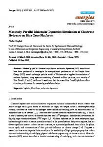
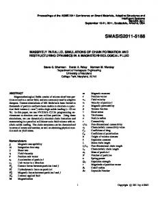
MPiSIM: Massively Parallel simulation tool for metallic system 187 where P x, P y and P z are the number of processors used on each direction. The number of link-cells on each processor is equally divided on each direction, since right now the density of the simulation system is quite uniform. To solve the big problem of spatial decomposition, load balance, we will enable user to specify the number of cells on each processor based on the estimated density distribution for next stage development. But this method still cannot automatically balance the load on each processor if the density changes dramatically during the simulation. Load balance problem is hard to overcome, if the density of simulation system is heterogeneous. 2.3. C OMMUNICATION METHOD Since link-cell is used, each cell should have its nearest 26 neighbor cells to build the neighbor list. For the link-cells on the boundary of each processor, it needs to shear the information of neighbor link-cell and atoms within them from the nearby processor. We will call these cells as sheared information zone, and the duplicated atoms as image atoms. Figure 1 shows communication mechanics in 2D. Let’s define the number of link-cell on each process as ncx , ncy and ncz . First, the communication is made along +x direction (east), means each processor sending atoms within the most east link-cells (ncy × ncz link-cells) into next processor then the communication is made along −x (west) direction. Secondly, the communication is done along y (north) direction, where the number of link-cell in communication is (ncx + 2)ncz , then the next communication is along y direction (south). Thirdly, the last communication is along z (up and down) direction and the number of link-cells in communication is (ncx + 2)(ncy + 2). After the communications along six directions, one cell is added in both directions of each of the three dimensions. As shown in Fig. 1, atom A and B are physically located on processor P0, and atom C is located on processor P1, after the communication, atom C has an image on processor P0 and so is B’s image on processor P1. To achieve periodic boundary condition (PBC), the atoms are shifted along the periodic direction before communication. For example, to apply periodic along x direction, we send the most east atoms in most east processors to the most west processor, after we added a displacement of ‘−Lx’ (Lx is the length of simulation box along x) for these atoms, and the ‘+Lx’ shift for the opposite direction. Periodic boundary condition is applied independently for each direction, to achieve PBC in OD, ID, 2D and 3D for simulations of clusters, wires, thin-films and bulk materials. Each processor is responsible for computing the forces and new positions for the atoms physically located on it. From Fig. 1 we can see that in each processor there two types of atoms, atom A, with its neighbors on the same processor, and atom B, with some of its neighbors located on the other processors, but having images of neighbors on the current processor. Not all of the information of the atoms needed to be communicated in every step. At each step the forces are calculated on each processor, and the position of atoms got updated, then the new positions of atoms in the sheared zone got passed to nearby processors, which means the image atoms position also got updated on each processor, prepared for the calculation at next step. For pair wise potential, like LJ and Morse, it is simple to only compute a force once for each pair of atoms, rather than once for each atom in the pair. EAM potential generally contain a two-body term and an electrical density term, which is also a function of summation of paired interaction between the given atom and its neighbors. Therefore the electrical density term calculation can still be treated it as a pair wise potential, which only need calculating once for

188 Y. Qi et al.

Figure 1. A schematic 2-D representation of the communication of atoms on the boundary of nearby processor and the link-cell neighbor search pattern used in domain decomposition program.

each pair of atoms. So only 13 neighbor cells have to be considered to construct the neighbor list for calculation of the energy and force. One thing special about EAM is that the electrical density term need to be updated in the sheared zone before the total energy and the accurate force on each atom can be calculated. So there are only one position communication in 2-body potential calculation, but two communications for density and position for EAM potential at each time step. D. Brown et al. has proposed a domain decomposition strategy by sending positions of atoms to nearby processors along 3 directions: east, south and above, then sending the force back along west, north and below, after the processor finishes the force calculation [10]. This method is suggested to minimize communication and avoid redundant force calculation. But the communication data of position and force along three directions almost has the same amount data of communicating only position along six directions. Even though the force only calculated on one processor, it needs extra space to accumulate forces for image atoms, and after the forces being send back, the combination of the force contributed from the same processor and nearby processors also takes time. Also a lock is added before all the forces being send back. We don’t know how much time Brown’s method will save, but it is hard to handle many-body force field calculation, where the force is not simply summation of atoms interaction. We think communication along 6 directions is more flexible for different types of potentials. In our design the communication is not based atom to atom, but cell to cell. A collection of atom information will be send together, while only a temporary array is needed for each communication. Only one global lock is added for summation of the total energy. 2.4. ATOMS REDISTRIBUTION To keep the neighbor list and link-cell methods working, we need update the atoms within the link-cell and redistribute the atoms to processor when some atoms diffuse away. We do this update every few timesteps, and assume that some atoms travel more than the skin distance,

MPiSIM: Massively Parallel simulation tool for metallic system 189 but less than the link-cell size. To avoid an all atoms communication between all the processors, we noticed that the only atoms on other processors can move into the current processor are the image atoms, which was in the nearby link-cells, and the only atoms can move out of the current processor are the atoms in the boundary link-cells. Since we kept the image atoms information from last link-cell update, we only need copy the moving in atoms from image atoms, and delete the moving out atoms. This method will save the communications time between nearby processors. 3. Performance test 3.1. E FFICIENCY OF MPiSIM The computation time at each time step contains three parts: the time of calculation of force and energy took place on each processor, which is linear scaled as Np, number of processors; the time cost on communication, which is proportional number of atoms in communication; and the time cost on the double calculation of energy of atoms on the boundary atoms, due to the duplication. If we assume the number of cells on each direction in every processor is equal, Nc, and the number of atoms in each cell is basically uniform, represented by D. We can write the time needed on each processor as T (Np) = T1 /Np + 13(3Nc2 − 3Nc + 8)Dτe + (3Nc2 + 3Nc + 8)Dτc ,

(1)

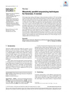
where Np is the number of processors, T1 is the time needed on only 1 processor, τc is the communication time per atom and τe is energy calculation time per atom. T1 scale linearly with the size of the simulation system, N, such that the dynamics time scales as N/Np. The second and third term in Eq. 1, are proportional to Nc2 D, where Nc is proportional to (N/Np)1/3, and D is independent of N and Np, so the communication time and duplication time scale as (N/Np)2/3. We cannot avoid time cost of communication and redundant force calculation, but the more cells on each processor, the more efficient the algorithm. 3.2. P ERFORMANCE ON ACL N IRVANA M ACHINE On ACL Nirvana Machine, we have tested our algorithm up to 512 processors. The first test is a series of 1000 steps EVN dynamics on system sizes range from 4000 to 1 024 000 Ni atoms, described by Sutton-Chen type of potential. In Figure 2-a, we showed the computational time of various sizes on 4 processors. Since we used the combination of link-cell and neighbor list method, the computational time scales O(N). The scaling performance of simulation size agrees well with the ideal linear scaling, represented by the solid line. In Fig. 2-b, we showed the simulation time scaling performance on different sizes of systems, and the dash line is the ideal linear scale of Np for system with 1 024 000 Ni atoms. The linear scale works well until 128 processors, then the computational time increased as processor number larger than 256 processors. Other groups who used the same machine have found the similar scaling behavior, which indicates this is a hardware related problem. The ACL Nirvana Machine consists of 16 SGI Origin 2000s each with 128 processors. The system interconnect is based on the HiPPI800 standard and is currently being upgraded to HiPPI 6400/GSN technology which will result in a bisection bandwidth of 25.6 Gbytes per second bi-directional. Since the communication time within the box is much faster than the communication between boxes, the performance beyond 128 processors is slowed down by the communication between processors in different

190 Y. Qi et al.

Figure 2. Scaling performance on ACL Nirvana Machine. (a) Scaling performance over size of the simulation system. The CPU time is for 1000 steps of NVE dynamics on four processors of Ni systems with Sutton–Chen many-body potential. (b) Scaling performance over Np, the number of processors used. The CPU time is for 1000 steps of NVE dynamics of Ni systems with Sutton–Chen many-body potential.

boxes. The more detailed discussion of communication time is not the focus of this paper. The scaling performance is not related to the potential employed in simulation. A scaling test on Ta, which used an EAM potential, showed the similar behavior. 3.3. P ERFORMANCE ON OTHER PLATFORMS Since we used the standard MPI library for information passing. The efficiency of MPiSIM is dependent of the MPI implementation on different platforms. We have tested MPiSIM on

MPiSIM: Massively Parallel simulation tool for metallic system 191

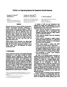
Figure 3. MpiSIM scaling over Np performance on various platforms, including Origin2000, HP Examplar X-classer, and Dell PC Beowulf cluster (wolf).

Origin 2000 (operating system is irix6.2 with MPI3.2 from SGI) machine in MSC, Caltech and NCSA, UIUC up to 16 processors, a Dell PC Beowulf cluster (operating system is Red Hat Linux 6.2 with LamMPI 6.3.2 from U. of Notre Dame) up to 12 processors, and HP Examplar X-class supercomputer (operating system is SPP-UX 5.3 with MPI from HP) in CACR, Caltech up to 16 processors. Due to the available resource we only test on these platforms up to maximum 16 processors. From our comparison in Fig. 3, the Origin 2000 gave the best linear scaling of Np. 4. Application The MPiSIM has been applied to various materials properties studies. At nano-scale simulations, we studied melting and crystallizations for Ni clusters range from hundreds to 8000 atoms, while two ranges have been captured. We also studied the dissociation, core energy, core structure, annihilation processes of screw dislocations in Ni. Other studies such as shock wave propagation in Ta and shear band formation in CuAg are carried on as well. 5. Summary MPiSIM, the massively paralleled simulation tool for metallic systems with various potentials have been developed and used on different applications. The portability on other machines can be easily done without modifying the code, due to the usage of MPI for parallelisation. But the best scaling results are on SGI origin 2000 based machines. In the near future the NPT dynamics and non-equilibrium MD (NEMD) will be implemented and more visualization tools and other utilities will be developed for analyzing the simulation results.

192 Y. Qi et al. Acknowledgements The author would thank E. F. Van de Velde for teaching ‘parallel scientific computation’, G. Wang and A. Strachan for implementing EAM potential for Ta, A. Strachan and D. Mainz for testing the code in LANL machines. This research was founded by a grant from DOE-ASCIASAP. The simulations were done in MSC, CACR, NCSA and ACL. The facilities of the MSC are also supported by grants from NSF (MRI CHE 99), ARO (MURI), ARO (DURIP), NASA, BP Amoco, Exxon, Dow Chemical, Seiko Epson, Avery Dennision, Chevron Corp., Asahi Chemical, GM, 3M and Beckman Institute. References 1. 2. 3. 4. 5. 6. 7. 8. 9. 10. 11. 12.

Abraham, F.F., Adv. Phys., 35 (1986) 1. Allen, M.P. and Tildesley, D.J., Computer Simulation of Liquids, Oxford, 1987. Heffelfinger, G.S., Comput. Phys. Commun., 128 (2000) 219. Boghosian, B.M., Comput. Phys. (1990) Computational Physics on the Connection Machines’. Plimpton, S., J. comput. Phys., 117 (1995) 1. Milstein, F., J. Appl. Phys., 44 (1973) 3825. Sutton, A.P. and Chen, J., Phil. Mag. Lett., 61 (1990) 139. Strachan, A., Cagin, T., Gulseren, O., Mukherjee, J., Cohen, K.E. and Goddard, W.A., III, Phys. Submitted, Rev. B. Gear, C.W., Numerical Initial Value Problems in Ordinary Differential Equations, Prentice-Hall, Englewood Cliffs, NJ, 1971. Brown, D. et al., Compt. Phys. Commun., 74 (1993) 67. Qi, Y., Cagin, T., Johnson, W.L. and Goddard, W.A., J. Chem. Phys., 115 (2001) 385. Qi, Y., Strachan, A., Cagin, T. and Goddard, W.A. III, Mat. Sci. Eng., 309–310 (2001) 156.