Computational Tool
MSMBuilder: Statistical Models for Biomolecular Dynamics Matthew P. Harrigan,1 Mohammad M. Sultan,1 Carlos X. Herna´ndez,2 Brooke E. Husic,1 Peter Eastman,1 Christian R. Schwantes,1 Kyle A. Beauchamp,3 Robert T. McGibbon,1,* and Vijay S. Pande1,2,4,5,* 1 Department of Chemistry and 2Program in Biophysics, Stanford University, Stanford, California; 3Memorial Sloan Kettering Cancer Center, New York, New York; and 4Department of Computer Science and 5Department of Structural Biology, Stanford University, Stanford, California
ABSTRACT MSMBuilder is a software package for building statistical models of high-dimensional time-series data. It is designed with a particular focus on the analysis of atomistic simulations of biomolecular dynamics such as protein folding and conformational change. MSMBuilder is named for its ability to construct Markov state models (MSMs), a class of models that has gained favor among computational biophysicists. In addition to both well-established and newer MSM methods, the package includes complementary algorithms for understanding time-series data such as hidden Markov models and time-structure based independent component analysis. MSMBuilder boasts an easy to use command-line interface, as well as clear and consistent abstractions through its Python application programming interface. MSMBuilder was developed with careful consideration for compatibility with the broader machine learning community by following the design of scikit-learn. The package is used primarily by practitioners of molecular dynamics, but is just as applicable to other computational or experimental time-series measurements.
INTRODUCTION Molecular dynamics (MD) is a powerful probe into atomistic dynamics. Recent advances in technology (e.g., specialized hardware (1) and commodity graphics-processing units (2)) and strategies (e.g., massively distributed architectures (3–5)) are enabling simulations to reach larger sizes and longer timescales. Increasing quantities of raw data require novel and sophisticated analysis techniques (6). Markov state models (MSMs) have gained favor for enabling researchers to draw interpretable conclusions from time-series data (6–9). Briefly, MSMs model dynamic systems using a set of discrete states and pairwise transition rates. From these models, the researcher can compute observables of interest and make predictions. These models are statistically rigorous and easy to interpret. Furthermore, MSMs are able to stitch together many independent simulation runs, allowing researchers to fully exploit distributed computing. Submitted July 29, 2016, and accepted for publication October 27, 2016. *Correspondence:
[email protected] or pande@ stanford.edu Kyle A. Beauchamp’s present address is Counsyl, Inc., South San Francisco, California. Robert T. McGibbon’s present address is D.E. Shaw Research, New York, New York. Editor: Bert de Groot. http://dx.doi.org/10.1016/j.bpj.2016.10.042 Ó 2017 Biophysical Society.
10 Biophysical Journal 112, 10–15, January 10, 2017
The idea of describing a system by its states and rates is natural for chemists and biologists, but the estimation of states and rates from finite data (perhaps MD) is not obvious. Since the introduction of MSMs to the biophysics community, algorithmic improvements for constructing MSMs and computing observables have been the focus of intense study. The practical implementation of these algorithms has spawned several historical packages for MSM construction (10–12). Each of these packages was tied strongly to the best practices in MSM construction at the time. Due to the fast-moving research involving MSMs, software rewrites were common (13,14). Here, we introduce MSMBuilder 3, a community-driven, open-source software package for constructing MSMs. MSMBuilder offers a curated selection of MSM construction algorithms based on modern advances in the field. MSMBuilder is implemented in the Python programming language with performance-critical components written in C. It employs an extensible application programming interface (API) modeled after that of scikit-learn. The modular design ensures that MSMBuilder 3 will be adaptable to future improvements in MSM construction. The package can be invoked directly from Python or via the command line. Through two instructive examples, we showcase the capabilities of MSMBuilder. In the first, we use MSMBuilder to analyze a biological system of interest from a data set
MSMBuilder
composed of more than 20,000 trajectories. This example builds a single MSM using methods that were unavailable in previous tools. Due to rapid advances in MSM methods, a variety of modeling choices are now available to researchers. In the second example, we demonstrate how MSMBuilder’s implementation of scoring functionals can be used to choose among these methods.
Instructive examples Constructing an MSM
MSMBuilder allows rapid analysis of large MD data sets. In this example, we construct an MSM of a kinase molecule. Kinases are critical enzymes that control cellular pathways. Malfunctions of kinases have been linked to many different cancers (15). Here, we use MSMBuilder to study the c-Src kinase, a regulator of cellular growth (16), and demonstrate that the resulting MSM can capture activation dynamics. Understanding the activation process provides atomistic, kinetic, and thermodynamic insights into the protein’s conformational heterogeneity, which can aid in the design of better therapeutics. Broadly, the procedure for constructing an MSM is to define a set of states and then estimate transition rates among those states. Before beginning model construction, researchers must obtain time-series data they wish to model. Usually, these data are the output of an MD engine (MSMBuilder supports nearly every MD trajectory file format (17)), but they could also be experimental time-series measurements. For this example, we use a previously generated MD data set for the c-Src kinase, publicly available from the Stanford Digital Repository (https://goo.gl/ LLchMT; for simulation details, see Shukla et al. (16)). The first step of model construction is to transform the raw Cartesian coordinates into vector features that are invariant to translation and rotation (Fig. 1, step 1). Here, we project our trajectory frames onto the dihedral angles created by each set of four consecutive a carbons (a angles) (18). This reduces the dimensionality of the data from 12,693 Cartesian coordinates to 518 features. The appropriate featurization depends on the particular system under study (see ‘‘Selecting hyperparameters’’ below). MSMBuilder offers a collection of featurization strategies with a unified interface. Popular features include backbone and side-chain dihedrals (through the DihedralFeaturizer class), heavy atom or Ca contact distances (ContactFeaturizer), the distance of reciprocal interatomic distances (DRIDFeaturizer) (19), and the root mean-square deviation of a set of structures (RMSDFeaturizer). There are additional utilities for concatenation of multiple choices of features and feature scaling. The second step in MSM construction projects structural features onto a lower-dimensional subspace (Fig. 1, step 2). This improves the statistical qualities of subsequent steps, but may discard important information if the projection is
FIGURE 1 Data transformations and their dimensionality. MSMs partition dynamical data into a set of states and estimate rates between them. A typical pipeline for state definition consists of a series of transformations (indexed by circled numbers) between representations of the data. Each step projects a higher-dimensional representation onto a lower-dimensional representation. The approximate dimension of each representation is reported below the representation name. Although it is not traditionally thought of as a dimensionality reduction, clustering (step 3) reduces each frame to a single integer cluster label. To see this figure in color, go online.
not carefully chosen. Time-structure based independent component analysis (tICA) finds a set of slow (high autocorrelation) coordinates. In practice, this dimensionality reduction has proven to be very useful for capturing slow, biophysical conformational changes (20,21). In this example, we reduce the dimensionality of our kinase data from 518 dihedrals to five tICA coordinates. MSMBuilder includes support for similar algorithms (e.g., SparseTICA (22)) as well as general manifold learning algorithms such as principal component analysis (PCA), SparsePCA, and MiniBatchSparsePCA. Before 2013, this step was not available for model construction. Accordingly, the software available at the time could not easily be extended to accommodate tICA intermediate processing. The design of MSMBuilder 3 permits arbitrary addition, subtraction, and reordering of data transformation steps. Next, we define the states of our MSM by grouping conformations that interconvert rapidly (Fig. 1, step 3). For the c-Src kinase, we employ the MiniBatchKMeans (23) clustering algorithm to partition our data into 200 microstates. We note that our data has been reduced from five tICA coordinates to one integer cluster label per frame. The prior dimensionality reduction permits the use of off-theshelf clustering algorithms. Accordingly, MSMBuilder supports K-means-like clustering algorithms (e.g., KCenters, KMedoids, and MiniBatchKMedoids) and hierarchical clustering. With our states defined, we proceed to estimate the rates among them. As the final model construction step, we learn a continuous-time MSM (24) from our labeled trajectories. We have chosen to use a continuous-time MSM to directly
Biophysical Journal 112, 10–15, January 10, 2017 11
Harrigan et al.
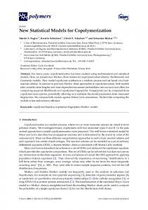
estimate transition rates; alternatively, we could have built a traditional MSM (to estimate transition probabilities) or a hidden Markov model (HMM). We direct interested readers to a more thorough application of HMM modeling to the c-Src data set in Ref. (25). The relevant Python code for constructing this MSM is shown in Fig. 2. Complete, executable code is available as Supporting Data in the Supporting Material as an IPython (26) notebook. To draw interpretable conclusions from our data via Markov modeling, we query the model. For c-Src, we use MSMBuilder to relate the model behavior to the biological function. In Fig. 3 a, we present a log-scaled, two-dimensional histogram of the trajectories projected onto the two dominant slow processes, or tICs, from our tICA model. We sampled the centroids of states (shown as pink and black stars) in low-free-energy regions to visualize representative configurations in three dimensions (27) (Fig. 3, c and d). The dominant tIC (x axis) highly correlates with the activation of the kinase. Kinase activation requires the unfolding of the activation loop (red) and an inward swing of the catalytic helix (C-helix). The inward rotation of the helix coincides with switching of the hydrogen-bonding pair from Glu-Arg to Glu-Lys (licorice). We investigated the dynamics among the active, inactive, and intermediate macrostates by applying robust Perron clustering analysis (PCCAþ) to our MSM. PCCAþ is a spectral clustering method that lumps MSM states into an arbitrary number of metastable macrostates, facilitating qualitative analysis
FIGURE 2 Sample MSM code. MSMBuilder balances a powerful API with ease of use. A sample workflow is shown here using the Python API. Following the successful model of the broadly applicable scikit-learn package, each modeling step is represented by an estimator object that operates on the data. Here, the AlphaAngleFeaturizer transforms raw coordinates into a angles. The output of this transformation is fed into the tICA dimensionality reduction, the MiniBatchKMeans clustering algorithm, and finally the ContinuousTimeMSM model. MSMBuilder provides a litany of utility functions for dealing with large MD data sets for input and output. Although this example shows the Python API, MSMBuilder is fully functional from the command line with an intuitive one-to-one correspondence between Python estimator objects and command-line commands. To see this figure in color, go online.
12 Biophysical Journal 112, 10–15, January 10, 2017
of rates and populations among biologically relevant macrostates (28). The rates among the three macrostates are shown by the thickness of arrows in Fig. 3 b. Further options for querying the model (not shown here, but available in MSMBuilder) include computation of relaxation timescales, transition path theory analysis (29–31), and generation of synthetic trajectories for visual inspection. The assortment of modeling options, such as the choice of featurizer, the use of dimensionality reduction, and the selection of the clustering algorithm, along with any associated internal parameter choices, presents the modeler with a motley of modeling decisions and tunable parameters. In the next section, we show how a scoring metric for MSMs can provide the modeler with an unbiased protocol for determining which parameters are suitable given a set of MD trajectories. Selecting hyperparameters Historically, the heuristic choice of hyperparameters (choices of protocol) rendered MSM construction as much of an art as a science. It is clear from the above section that an abundance of algorithms are available in MSMBuilder. In this instructive example, we use a scoring functional to select the best models. N€uske et al. (32) introduced a variational principle that formalized the definition of a good MSM. In keeping with inspiration from the broader machine learning community, MSMBuilder extends this formalism in the context of cross-validation through the work of McGibbon and Pande (33). The resulting generalized matrix Rayleigh quotient (GMRQ) score offers an objective way to pick the best model (i.e., the appropriate modeling choices) from the given data. Briefly, the GMRQ measures the ability of a model to capture the slowest dynamics of a system. According to the variational principle, approximating the full phase space by discrete states will always yield dynamics that are too fast. The GMRQ score is a summation of the leading eigenvalues of the model and therefore provides a measure of slowness. A higher score means the model is closer to the variational bound and therefore should be preferred over lower-scoring models. In this example, we use the GMRQ score under crossvalidation to evaluate the relative merit of enumerated hyperparameter values when constructing a model for the Fs peptide (34). The relevant code in Fig. 4 sets up a choice between two structural features (dihedral angles or contact distances) and a choice among tICA lag times. We perform shuffle-split cross-validation by randomly assigning the 28 trajectories to either the training set or the test set. The MSM is learned on the training set and scored on the test set. By concealing the training data during scoring, cross-validation guards against overfitting (overconfidence in excessively complex models). The trajectories are reshuffled and this process is repeated to compute an average
MSMBuilder
FIGURE 3 c-Src kinase MSM. MSMBuilder constructs interpretable models from large data sets. (a) This figure shows a two-dimensional histogram for the Src kinase from a tICA-MSM analysis projected onto the dominant modes of a tICA model. (b) A simple macrostate model of the dynamics shows the presence of an intermediate state, I1, connecting the inactive and active states. The arrow thickness corresponds to the rate of transition. The model indicates that the active state (red) is the most stable state, followed by the inactive (gray) and intermediate (blue) states. The analysis discovers a coordinate (the first tIC) between the known active and inactive conformations. Representative structures are selected from MSM states and show the conformational differences between the two basins. (c and d) The unfolding of the activation loop (red helix) forms a catalytically active Src that is capable of initiating and regulating downstream signaling pathways. To see this figure in color, go online.
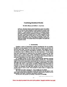
score for a given set of hyperparameters. The scores for each of the 50 cross-validation splits are plotted in a box plot in Fig. 5. The dihedral angle featurization with a lag time of four steps gives the best model in this search space. A
FIGURE 4 Sample GMRQ code. MSMBuilder seamlessly interoperates with the broader Python ecosystem. In this code sample, we use scikit-learn for algorithm-agnostic data processing and MSMBuilder for biophysicsoriented time-series algorithms with the goal of selecting model hyperparameters. Our analysis pipeline is similar to that described in ‘‘Constructing an MSM’’ but with a choice of features (between dihedrals and contact distances) and tICA lag times (among 1, 4, 16, and 64 steps). The ShuffleSplit cross-validation scheme runs 50 iterations of equal partitioning of the 28 trajectories between train and test sets, and we perform a full grid-search over parameter choices. We can plot the distribution of scores versus parameters as in Fig. 5. To see this figure in color, go online.
simple grid search as performed in this example can become intractable as the number of hyperparameters (i.e., the dimension of the search space) increases. We direct interested users to Osprey (35), a tool for hyperparameter optimization that includes a variety of search strategies and support for parallel computation. Osprey interoperates with any scikit-learn estimator, including those in MSMBuilder. This example leverages the Pipeline, ShuffleSplit, and GridSearchCV machinery from scikit-learn. Additionally, MSMBuilder uses this library internally for generic machine learning algorithms such as clustering and PCA. We note that such general algorithms do not need to be reinvented and reprogrammed by the biophysics community. By taking advantage of this widely used machine learning library, we ensure that the development of MSMBuilder is focused on biophysical algorithms and considerations. This will enable rapid adoption of the latest algorithms that have demonstrated an improved ability to build MSMs (e.g., (33)) and a larger community for code maintenance and longevity.
CONCLUSION MSMBuilder 3 is a powerful and accessible software package for drawing interpretable conclusions from time-series data. We use two examples to demonstrate how MSMBuilder
Biophysical Journal 112, 10–15, January 10, 2017 13
Harrigan et al.
FIGURE 5 GMRQ parameter selection. MSMBuilder offers robust machinery for selecting hyperparameters that cannot a priori be learned from the data. Here, we perform shuffle-split cross-validation over choices of featurization and tICA lag time. Historically, these parameters were chosen heuristically. With the advent of the GMRQ score and its implementation in MSMBuilder, we can choose these parameters in a statistically rigorous way. Here, we plot the distribution of scores for each set of model parameters. Note that a higher score is generally an indication of a more predictive model. In this example, we find that featurization with dihedral angles at a lag time of four steps has the highest median score, and recommend this hyperparameter set to be chosen for the final model. To see this figure in color, go online.
can make sense of an MD data set consisting of thousands of trajectories in a highly automated and statistically robust way. In the first example, we construct a ‘‘vanilla’’ MSM and show how MSMBuilder enables the construction of interpretable models that expose the connection between biological function and structural dynamics. We highlight the breadth of relevant algorithmic choices for featurization, normalization, dimensionality reduction, clustering, and MSM modeling. In the second instructive example, we acknowledge that the explosion of choices in parameters and protocol can be overwhelming. We use the GMRQ score and off-the-shelf cross-validation machinery to do a simple grid search over tunable parameters to evaluate the relative merit of many MSMs built on the same MD data set of a small protein. Since cross-validation is not a technique unique to biophysics, we leverage the greater Python machine learning ecosystem for this example. More broadly, MSMBuilder’s power and clarity are derived from its integration with the machine learning community at large. Our ability to focus on developing methods specifically designed for biophysics and time-series analyses comes from exploiting general-purpose algorithms implemented by respective experts. The clarity of MSMBuilder’s API is due in large part to the massive amount of effort and skill put into the design of scikit-learn’s API. As distributed computing and Markov modeling continue to become more prominent, MSMBuilder will offer a sustainable, extensible, powerful, and easy-to-use set of Python and command-line tools to help researchers draw meaningful conclusions from their data.
14 Biophysical Journal 112, 10–15, January 10, 2017
MSMBuilder documentation and installation are available at http://msmbuilder.org. The source code is available under the open-source LGPL2.1 license and is accessible at http://github.com/msmbuilder/msmbuilder. The current release at the time of this writing is version 3.5 (36). Complete examples can be found as IPython notebooks in the Supporting Data and at http://github.com/msmbuilder/ paper. SUPPORTING MATERIAL Supporting Data are available at http://www.biophysj.org/biophysj/ supplemental/S0006-3495(16)31048-7.
AUTHOR CONTRIBUTIONS M.P.H., M.M.S., C.X.H., and B.E.H. wrote the manuscript. M.P.H., M.M.S., C.X.H., B.E.H., P.E., C.R.S., K.A.B., R.T.M., and V.S.P. edited the manuscript. M.P.H., M.M.S., C.X.H., B.E.H., P.E., C.R.S., K.A.B., and R.T.M. wrote the software. V.S.P. supervised the project.
ACKNOWLEDGMENTS We thank all of our contributors, including Stephen Liu, Patrick Riley, Steven Kearnes, Joshua Adelman, and Gert Kiss. We also thank members of the Chodera, Pande, and Noe´ labs for helpful discussions, and Ariana Peck for invaluable feedback on the manuscript. This work was supported by National Institutes of Health grants U19 AI109662 and 2R01GM062868. M.M.S. received support from National Science Foundation grant MCB-0954714. C.X.H. received support from the National Science Foundation Graduate Research Fellowship Program
MSMBuilder (DGE-114747). K.A.B. received support from National Institutes of Health grant P30CA008747, the Sloan Kettering Institute, and Starr Foundation grant I8-A8-058. K.A.B. is currently an employee of Counsyl, Inc. R.T.M. is currently an employee of D.E. Shaw Research, LLC. V.S.P. is a consultant and SAB member of Schrodinger, LLC and Globavir, sits on the Board of Directors of Omada Health, and is a General Partner at Andreessen Horowitz.
17. McGibbon, R. T., K. A. Beauchamp, ., V. S. Pande. 2015. MDTraj: a modern open library for the analysis of molecular dynamics trajectories. Biophys. J. 109:1528–1532.
REFERENCES
20. Schwantes, C. R., and V. S. Pande. 2013. Improvements in Markov state model construction reveal many non-native interactions in the folding of NTL9. J. Chem. Theory Comput. 9:2000–2009.
1. Shaw, D. E., M. M. Deneroff, ., S. C. Wang. 2008. Anton, a specialpurpose machine for molecular dynamics simulation. Commun. ACM. 51:91. 2. Friedrichs, M. S., P. Eastman, ., V. S. Pande. 2009. Accelerating molecular dynamic simulation on graphics processing units. J. Comput. Chem. 30:864–872. 3. Shirts, M., and V. S. Pande. 2000. COMPUTING: screen savers of the world unite! Science. 290:1903–1904. 4. Buch, I., M. J. Harvey, ., G. De Fabritiis. 2010. High-throughput allatom molecular dynamics simulations using distributed computing. J. Chem. Inf. Model. 50:397–403. 5. Kohlhoff, K. J., D. Shukla, ., V. S. Pande. 2014. Cloud-based simulations on Google Exacycle reveal ligand modulation of GPCR activation pathways. Nat. Chem. 6:15–21. 6. Schwantes, C. R., R. T. McGibbon, and V. S. Pande. 2014. Perspective: Markov models for long-timescale biomolecular dynamics. J. Chem. Phys. 141:090901. 7. Pande, V. S., K. Beauchamp, and G. R. Bowman. 2010. Everything you wanted to know about Markov state models but were afraid to ask. Methods. 52:99–105. 8. Chodera, J. D., and F. Noe´. 2014. Markov state models of biomolecular conformational dynamics. Curr. Opin. Struct. Biol. 25:135–144. 9. G. R. Bowman, V. S. Pande, and F. Noe´, editors 2014. An Introduction to Markov State Models and Their Application to Long Timescale Molecular Simulation. Springer, New York. 10. Bowman, G. R., X. Huang, and V. S. Pande. 2009. Using generalized ensemble simulations and Markov state models to identify conformational states. Methods. 49:197–201. 11. Beauchamp, K. A., G. R. Bowman, ., V. S. Pande. 2011. MSMBuilder2: modeling conformational dynamics at the picosecond to millisecond scale. J. Chem. Theory Comput. 7:3412–3419. 12. Senne, M., B. Trendelkamp-Schroer, ., F. Noe´. 2012. EMMA: a software package for Markov model building and analysis. J. Chem. Theory Comput. 8:2223–2238. 13. Scherer, M. K., B. Trendelkamp-Schroer, ., F. Noe´. 2015. PyEMMA 2: a software package for estimation, validation, and analysis of Markov models. J. Chem. Theory Comput. 11:5525–5542. 14. Doerr, S., M. J. Harvey, ., G. De Fabritiis. 2016. HTMD: highthroughput molecular dynamics for molecular discovery. J. Chem. Theory Comput. 12:1845–1852.
18. Flocco, M. M., and S. L. Mowbray. 1995. C alpha-based torsion angles: a simple tool to analyze protein conformational changes. Protein Sci. 4:2118–2122. 19. Zhou, T., and A. Caflisch. 2012. Distribution of reciprocal of interatomic distances: a fast structural metric. J. Chem. Theory Comput. 8:2930–2937.
21. Pe´rez-Herna´ndez, G., F. Paul, ., F. Noe´. 2013. Identification of slow molecular order parameters for Markov model construction. J. Chem. Phys. 139:015102. 22. McGibbon, R. T., and V. S. Pande. 2016. Identification of simple reaction coordinates from complex dynamics. arXiv:1602.08776. 23. Sculley, D. 2010. Web-scale K-means clustering. Proc.19th Int. Conf. World Wide Web. Association for Computing Machinery. 24. McGibbon, R. T., and V. S. Pande. 2015. Efficient maximum likelihood parameterization of continuous-time Markov processes. J. Chem. Phys. 143:034109. 25. McGibbon, R. T., B. Ramsundar, ., V. S. Pande. 2014. Understanding protein dynamics with L1-regularized reversible hidden Markov models. Proc. 31st Int. Conf. Machine Learning. 1197–1205. 26. Pe´rez, F., and B. E. Granger. 2007. IPython: a system for interactive scientific computing. Comput. Sci. Eng. 9:21. 27. Humphrey, W., A. Dalke, and K. Schulten. 1996. VMD: visual molecular dynamics. J. Mol. Graph. 14:33–38, 27–28. 28. Deuflhard, P., and M. Weber. 2005. Robust Perron cluster analysis in conformation dynamics. Linear Algebra Appl. 398:161–184. 29. Metzner, P., C. Sch€utte, and E. Vanden-Eijnden. 2009. Transition path theory for Markov jump processes. Multiscale Model. Simul. 7:1192– 1219. 30. Berezhkovskii, A., G. Hummer, and A. Szabo. 2009. Reactive flux and folding pathways in network models of coarse-grained protein dynamics. J. Chem. Phys. 130:205102. 31. Noe´, F., C. Sch€utte, ., T. R. Weikl. 2009. Constructing the equilibrium ensemble of folding pathways from short off-equilibrium simulations. Proc. Natl. Acad. Sci. USA. 106:19011–19016. 32. N€uske, F., B. G. Keller, ., F. Noe´. 2014. Variational approach to molecular kinetics. J. Chem. Theory Comput. 10:1739–1752. 33. McGibbon, R. T., and V. S. Pande. 2015. Variational cross-validation of slow dynamical modes in molecular kinetics. J. Chem. Phys. 142:124105. 34. McGibbon, R. T. 2014. Fs MD trajectories. https://figshare. com/articles/Fs_MD_Trajectories/1030363. http://dx.doi.org/10.6084/ m9.figshare.1030363.v1.
15. Taylor, S. S., and A. P. Kornev. 2011. Protein kinases: evolution of dynamic regulatory proteins. Trends Biochem. Sci. 36:65–77.
35. McGibbon, R. T., C. X. Herna´ndez, ., V. S. Pande. 2016. Osprey 1.0.0. https://zenodo.org/record/56251. http://dx.doi.org/10. 5281/zenodo.56251.
16. Shukla, D., Y. Meng, ., V. S. Pande. 2014. Activation pathway of Src kinase reveals intermediate states as targets for drug design. Nat. Commun. 5:3397.
36. McGibbon, R. T., M. Harrigan, ., G. Kiss. 2016. MSMBuilder 3.5. https://zenodo.org/record/55601. http://dx.doi.org/10.5281/zenodo. 55601.
Biophysical Journal 112, 10–15, January 10, 2017 15