Multi-Attribute Decision Making Using Hypothetical ... - CiteSeerX

Multi-Attribute Decision Making Using Hypothetical Equivalents and Inequivalents

Tung-King See Graduate Research Assistant e-mail: [email protected]

Ashwin Gurnani Graduate Research Assistant e-mail: [email protected]

Kemper Lewis

In this paper, the problem of selecting from among a set of alternatives using multiple, potentially conflicting criteria is discussed. A number of approaches are commonly used to make these types of decisions in engineering design, including pairwise comparisons, ranking methods, rating methods, weighted sum approaches, and strength of preference methods. In this paper, we first demonstrate the theoretical and practical flaws with a number of these commonly employed methods. We demonstrate the strengths and weaknesses of the various decision-making approaches using an aircraft selection problem. We then present a method based on the concept of hypothetical equivalents and expand the method to include hypothetical inequivalents. Visualization techniques, coupled with an indifference point analysis, are then used to understand the robustness of the solution obtained and determine the appropriate additional constraints necessary to identify a single robust optimal alternative. The same aircraft example is used to demonstrate the method of hypothetical equivalents and inequivalents. 关DOI: 10.1115/1.1814389兴

1

Associate Professor e-mail: [email protected] Department of Mechanical and Aerospace Engineering, University of Buffalo, 1010 Furnas Hall, Buffalo NY 14260

1

Introduction

There are always trade-offs in decision making. We have to pay more for better quality, carry around a heavier laptop if we want a larger display, or wait longer in a line for increased airport security. More specifically, in engineering design, we can be certain that there is no one alternative that is best in every dimension. Therefore, how to make the ‘‘best’’ decision when choosing from among a set of alternatives in a design process has been a common problem in research and application in engineering design. When the decision is multiattribute in nature, common challenges include aggregating the criteria, rating of the alternatives, weighting of the attributes, and modeling strength of preferences in the attributes. In recent years, decision-based design has proposed that decisions such as these are a fundamental construct engineering design 关1–3兴. In general, the multiattribute decision problem can be formulated as follows: Choose an alternative i, n

maximize

兺wr

(1)

兺 w ⫽1

(2)

V i⫽

j ij

j⫽1

n

subject to

j⫽1

j

where V is the value function for alternative i, w is the weight for attribute j, and r is the normalized score for alternative i on attribute j. There are many ways to implement and solve this formulation. Most methods focus on formulating the attribute weights w j and/or the alternative scores r i j indirectly or directly from the decision maker’s preferences. In new product development, a common challenge in a design process is how to capture the preferences of the end-users while also reflecting the interests of the designer共s兲 and producer共s兲. Typically, preferences of endusers are multidimensional and multiattribute in nature. If companies fail to satisfy the preferences of the end-user, the product’s potential in the marketplace will be severely limited. For example, the Ford Motor Company selected and introduced the Edsel and 1 To whom correspondence should be addressed. Contributed by the Design Automation Committee for publication in the JOURNAL OF MECHANICAL DESIGN. Manuscript received April 3, 2003; revised March 17, 2004. Associate Editor: J. Renaud.

950 Õ Vol. 126, NOVEMBER 2004

lost more than $100 million. General Motors was forced to abandon its Wankel Rotary Engine after over $100 million had been invested in the project 关4兴. At some point in Ford’s and GM’s design process, the decision of selecting these concepts was deemed to be sound and effective. However, good decisions have also been made that are successful. For example, Southwest Airlines’ decision to only select the 737 aircraft for the entire fleet was excellent, as it lowered the maintenance and training costs. While the specific process used by these companies to make these selection decisions is not in the scope of this paper, we hypothesize that perhaps the process being used to make selection decisions impacts the outcome more than the information used in the decision. In fact, studies have shown this to be true, as when the number of alternatives approaches seven, the process used to make the decision influences the outcome 97% of the time 关5兴. In addition, it is difficult to evaluate the value of a decision based on the outcome itself. Rather, the process being used should be used as the evaluation and validation standard 关6兴. In this paper, we attempt to demonstrate the effect of a decision process on the outcome and present a method that facilitates the practical selection from among a set of alternatives using theoretically sound decision theory principles. In the next sections, we use a simple example to present the strengths and weaknesses of common decision-making processes: pairwise comparison, ranking, rating/normalization, strength of preferences, and the weighted sum method. We then present the method of hypothetical equivalents and inequivalents 共HEIM兲. In the latter half of the paper, we present an investigation of the aircraft case study using HEIM.

2

Multiattribute Decision Methods

In this section, a number of common approaches are used to solve the following multiattribute decision problem. For illustration purposes, suppose a fictional airline carrier, Jetair, is planning to establish an air fleet to serve the routes on major cites among Asia Pacific countries and the United States. Jetair has decided to purchase only one type of aircraft for its entire fleet to reduce operating cost, similar to the strategy used by Southwest Airlines and Jetblue Airway 关7兴. At this point, Jetair has identified four possible choices that meet Jetair’s requirements and budget constraints: Boeing 777-200 共long range兲, Boeing 747-200, Airbus 330-200, and Airbus 340-200. After reflecting upon the appeal of each of the four aircraft, Jetair has identified three key attributes:

Copyright © 2004 by ASME

Transactions of the ASME

Table 1 Attribute data for aircraft alternatives

Table 2 Results of ranking procedure

Attribute Aircraft B777-200 共long range兲 B747-200 A330-200 A340-200

Attribute

Speed 共Mach兲

Max. cruise range 共nmi兲

No. of passengers

0.84

8820

301

0.85 0.85 0.86

6900 6650 8000

366 253 239

1. The number of passengers the plane can hold, which obviously reflects revenue for each flight. 2. The cruise range, where a longer cruise range will provide passengers with nonstop service. 3. The cruise speed, where a faster cruise speed means shorter times needed for each flight. Potentially, this could increase the frequency of turnaround times. In Table 1, the data of the three attributes for the four aircraft 关8,9兴 are given. This problem is simplistic and is not meant to be realistic of how airliners choose which aircraft to purchase. It is meant to illustrate the practical and theoretical advantages and disadvantages when using common decision-making methods to make selection decisions from among a set of alternatives in a multicriteria environment. 2.1 Pairwise Comparisons. Jetair first uses a pairwise comparison to make their decision, first comparing B777 with B747 attribute by attribute, and then choosing the aircraft that ‘‘wins’’ on the most attributes. This process is repeated taking the ‘‘winner’’ of the previous comparison and comparing with the next alternative. This process is similar to any kind of tournament approach to determine the winner from among many competitors. More generally, the pairwise comparison method takes two alternatives at a time and compares them to each other. A pairwise approach is used in the analytic hierarchy process 共AHP兲 to find relative importances among attributes 关10兴. Adaptations of AHP and other pairwise methods are widely used to obtain relative attribute importances 关11兴, to select from competing alternatives 关12兴, and to aggregate individual preferences 关13,14兴. Ordinal-scale comparison is used in this problem. Thus, the B747 is better than the B777 because the B747 has a higher maximum speed and a greater passenger capacity. Next, the B747 is then compared to the A330 and is preferred because of a longer cruise range and greater passenger capacity. However, the A340 is preferred over the B747 because of the greater speed and cruise range. Thus, Jetair concludes that the A340 is the superior aircraft for its needs. However, if Jetair compares the A340 with the B777, B777 is the preferred aircraft. Thus, Jetair’s decision process will produce the following rankings, where ‘‘Ɑ’’ indicates ‘‘preferred to’’: B747ⱭB777ⱭA340ⱭB747 which is a set of intransitive preferences that will lead to decision cycling 关15兴. There are two fundamental flaws in this method: • It ignores strength of preference: suppose aircraft E is just a little better than aircraft F on two out of three attributes, but much worse on the third attribute. Clearly, most airliners would disregard aircraft E, but pairwise comparisons ignore this information. • This procedure ignores the relative important of the attributes: in AHP, pairwise comparisons are used to find relative importances, but then the problems with pairwise comparisons to choose among alternatives only increase. Journal of Mechanical Design

Aircraft

Speed 共Mach兲

Max. range 共nmi兲

No. of passengers

Total score

B777-200 B747-200 A330-200 A340-200

1 2.5 2.5 4

4 2 1 3

3 4 2 1

8 8.5 5.5 8

Further details regarding the theoretical problems with pairwise comparisons can be found in Refs. 关5, 16, 17兴. In the next section, a ranking method is used to make the same decision. 2.2 Ranking of Alternatives. Rankings are commonly used to rank order a set of alternatives. U.S. News and World Report annually ranks colleges based upon a number of attributes 关18兴. The NCAA athletic polls are based on a ranking system. Compared to pairwise methods, ranking methods are slightly more elaborate. However, ranking methods still make limiting assumptions and are limited in applicability in engineering design. Suppose Jetair uses the data from Table 1 and ranks the alternatives with respect to each attribute. Jetair assigns four points for the top ranked alternative for a given attribute, three points for second, two points for third, and one point for the worst. For a tie, Jetair averages the points. Table 2 shows the results of this procedure. The preferred aircraft using this method is B747 with 8.5 points; while B777 and A340 follow closely behind it with 8 points. A330 is clearly a noncontender. Noncontenders are alternatives that are equal to or worse than at least one other alternative with respect to every attribute. Therefore, the A330 alternative can be dropped from consideration, since it should never be picked. Making the rational decision to drop the A330 from contention, the resulting rankings are shown in Table 3. As shown in Table 3, all three alternatives are tied. There is no clear preferred aircraft. This outcome has demonstrated that the ranking procedure has violated the independence of irrelevant alternatives 共IIA兲 principle, which states that the option chosen should not be influenced by irrelevant alternatives or clear noncontenders 关19兴. If a noncontender exists, it would never be rational to choose this alternative. Further, although it is not shown here, noncontenders can be included to make any of the alternatives 共except A330兲 win. Ranking methods, while violating the IIA principle, also assume linear preference strengths. That is, the difference between first and second place is the same as the difference between fourth and fifth and so on. In the next section, a rating procedure is used for the same problem. 2.3 Normalization Rating. When aggregating attributes that have different units of measure, normalization is a common way to eliminate dimensions from the problem. Since in the problem of Table 1, the dimensions for all three attributes are different, normalization could certainly convert these attributes into a dimensionless scale, so they can be aggregated. Assume a simple linear method to normalize the aircraft attribute data on a scale from 0 to 100 where 0 is assigned to the Table 3 Rankings without the A330 Attribute Aircraft

Speed 共Mach兲

Max. range 共nmi兲

No. of passengers

Total score

B777-200 B747-200 A340-200

1 2 3

3 1 2

2 3 1

6 6 6

NOVEMBER 2004, Vol. 126 Õ 951

Table 4 Normalized alternative scores

Table 5 Strength of preference assessments

Attribute

Attribute

Aircraft

Speed 共Mach兲

Max. range 共nmi兲

No. of passengers

Total score

Aircraft

Speed 共Mach兲

Max. range 共nmi兲

No. of passengers

Total score

B777-200 B747-200 A330-200 A340-200

0 50 50 100

100 11.5 0 62.2

48.8 100 11 0

148.8 161.5 61.0 162.2

B777-200 B747-200 A330-200 A340-200

0 35 35 100

100 50 0 80

35 100 5 0

135 185 40 180

worst value and 100 to the best value, is used as shown in the following: Speed 共Mach兲: Range 共nmi兲: No. of passengers:

0.84⫽0 points 0.86⫽100 points 6650⫽0 points 8820⫽100 points 239 passengers⫽0 points 366 passengers⫽100 points

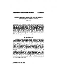
The intermediate values for each attribute are calculated using linear interpolation. Table 4 shows the normalized scale for the example. We can now sum the individual ratings for each alternative since all the attributes are on the same scale. By doing this, the A340 is determined to be the preferred aircraft. As opposed to a ranking procedure 共Section 2.2兲, normalized ratings do satisfy the independence of irrelevant alternatives principle because the noncontenders do not affect the relative scores. However, these normalized values depend on the relative position of the attributes value within the range of values. The lack of a rigorous method to determine the normalizing range leads to paradoxes 关3兴. Further, this procedure still neglects the strength of preference within each attribute. Ignoring the strength of preferences can lead to a result that does not reflect the decision maker共s兲 preferences. In addition, relative importances of the attributes are not used. While weights could certainly be assigned to each attribute 共in Table 4 it is assumed that all the weights are equal兲 and then used to determine the final score, this creates further complications as shown in the next section. 2.4 Strength of Preferences and Weighted Sums. Using a linear preference scale may not truly reflect a decision maker’s preferences. Jetair would be better off using a nonlinear strength of preference representation, better reflecting their true preferences. In this paper, simple assumptions are made for illustration purposes. For the cruise speed, assume that an increase from 0.85 to 0.86 is preferred to an increase from 0.84 to 0.85. For the aircraft range, assume an increase from 6500 to 7000 nmi is more preferred than an increase from 8000 to 9000 nmi 共because if the cruise range is less than 7000 nmi, the aircraft may have to make multiple stops for refueling兲. For the number of passengers assume that an increase from 290 to 340 is slightly preferred over an increase from 240 to 290. There are a number of ways to assess

the strength of preferences, including utility theory methods 关3,20,21兴. These strength of preferences are shown, respectively, in Figs. 1共a兲, 共b兲, and 共c兲. Table 5 shows the numerical values for each attribute according to these strength of preference functions as well as the aggregation of scores for each alternative. Here, B747 is the winner with 185 points and is followed closely by A340 with 180 points. Even though using strength of preferences more accurately represents decision makers’ preferences and does not violate the IIA principle, determining the relative importance of the attributes is largely an arbitrary process. This arbitrary process can create a number of complications in multiattribute decision making and optimization 关22–25兴, some of which are discussed here. First, suppose that Jetair has decided that cruise range is the most important attribute, followed by the numbers of passengers and then the speed. Therefore, Jetair has decided to use the weights, 0.1, 0.6, and 0.3, respectively, for speed, range, and passengers. Using these weights and Eq. 共1兲, the B777 aircraft is determined to be the winner, as shown in Table 6. Note that the preference strengths shown in Table 5 are also used here. Suppose that some time later 共maybe even after the first decision has been made兲, Jetair has decided that the number of passengers is the most important attribute and not the cruise range, or decided to use a moderate set of weights. Undeniably, a different set of weights leads to a different preferred aircraft as shown in Table 7. As shown in Tables 6 and 7, different sets of weight can lead to very different results. This dependence on a largely arbitrary assessment of weights that can fluctuate is the primary drawback of using any method where weights are not chosen using strict decision theory principles 关26兴. In the next section, a more rigorous method, called hypothetical equivalents, to find a theoretically correct set of weights based upon a decision maker’s stated preferences is discussed. This method is applied to the aircraft selection problem. 2.5 Hypothetical Equivalents. The hypothetical equivalents approach determines the attribute weights using a set of preferences rather than selecting weights arbitrarily based on intuition or experience. While first encountered in the management literature 关27兴, in this paper it is developed and expanded for design decisions. The approach is based on developing a set of hypothetical alternatives that the decision maker is indifferent between. In other words, it is based on identifying hypothetical alternatives

Fig. 1 Strength of preference for cruise speed, range, and number of passengers

952 Õ Vol. 126, NOVEMBER 2004

Transactions of the ASME

Table 6 Results for weights of †0.1,0.6,0.3‡

Table 10 Results using hypothetical equivalents

Attribute and weights

Attribute and weights

Aircraft

0.1 Speed 共Mach兲

0.6 Max. range 共nmi兲

0.3 No. of passengers

Value

B777-200 B747-200 A330-200 A340-200

0 35 35 100

100 50 0 80

35 100 5 0

70.5 63.5 5 58

that have equal value to the decision maker. These indifference points are then used to analytically solve for the theoretically correct set of attribute weights. The approach is best illustrated through use of an example. Suppose that Jetair felt uncomfortable assessing weights directly, and therefore, started by considering a number of hypothetical choices. These hypothetical choices can be developed by the decision maker in order to meet the indifference requirement and are shown in Table 8 for this problem. Assume that Jetair is indifferent between aircraft A and B. That is both aircraft are equivalent to them and it would not matter which one they chose. Based on the strength of preferences that are used in Section 2.4, aircraft A is at the bottom of the range on both speed and range, but at the top in terms of number of passengers. Aircraft B is at the bottom on range and number of passengers, but at the top in terms of speed. Therefore, by saying they are indifferent between aircraft A and aircraft B, the total value 共represented by the total score in Table 9兲 must be equal, which gives Eq. 共3兲: w 1 ⫽w 3

(3)

Since there are three attributes, three weights must be solved for. This requires three equations, Eq. 共3兲 being one of them. Another equation is generated from the fact that the weights are normalized and sum to one:

Table 7 Results for various weight combinations Attribute weights 共speed, range, no. of passengers兲

Preferred aircraft

共0.2,0.2,0.6兲 共0.3,0.4,0.3兲

B747 A340

Table 8 Hypothetical aircraft choices Attribute and weights

Aircraft Aircraft Aircraft Aircraft Aircraft

A B C D

w1 Speed 共Mach兲

w2 Max. range 共nmi兲

w3 No. of passengers

0.84 0.86 0.84 0.86

6650 6650 8820 6900

300 250 250 300

Table 9 Normalized scores for hypothetical aircraft Attribute and weights w1 w2 w3 Speed Max. range No. of 共Mach兲 共nmi兲 passengers

Aircraft Aircraft Aircraft Aircraft Aircraft

A B C D

0 100 0 100

0 0 100 50

Journal of Mechanical Design

100 0 0 100

Value 100W3 100W1 100W 2 100W 1 ⫹50W 2 ⫹100W 3

Aircraft

1/6 Speed 共Mach兲

2/3 Max. range 共nmi兲

1/6 No. of passengers

Value

B777-200 B747-200 A330-200 A340-200

0 35 35 100

100 50 0 80

35 100 5 0

72.5 55.8 6.7 70.0

w 1 ⫹w 2 ⫹w 3 ⫽1

(4)

Therefore, one more indifference point must be found in order to generate the third equation. Assume that Jetair is indifferent between aircraft C and aircraft D. Using the strength of preferences in Sec. 2.4, the total scores for each aircraft are shown in Table 9. This indifference point results in the following equation: 100w 1 ⫹50w 2 ⫹100w 3 ⫽100w 2 or 2 共 w 1 ⫹w 3 兲 ⫽w 2

(5)

Together, solving Eqs. 共3兲, 共4兲, and 共5兲 give w 1 ⫽1/6 w 2 ⫽2/3 w 3 ⫽1/6 With these attribute weights, a weighted sum result using the strength of preferences from Sec. 2.4 is shown in Table 10. The preferred aircraft is B777. The concept of indifferent points is also used in other decisionmaking contexts. In utility theory, one method to construct utility functions queries a decision maker for their indifference point between whether or not to accept a guaranteed payoff or play a lottery for a chance at a potentially larger or smaller payoff 关28兴. In Ref. 关29兴 indifference relationships are used to determine preferences that are then used to solve for weights and compensation strategies. While other work on indifference points uses lottery probabilities or preferences to find relative importances among attributes, hypothetical alternatives utilize product alternatives and their attributes directly. However, finding hypothetical equivalents that are exactly of equivalent value to a decision maker, or ‘‘indifference points,’’ can be a challenging and time-consuming task 关30兴, specifically in the context of constructing utility functions. Therefore, the hypothetical equivalents method is expanded to a more general approach that is easier to apply to complex decisions, called the hypothetical equivalents and inequivalents method 共HEIM兲, which is explained in the next section.

3 An Appoach to Decision Making Using Hypothetical Equivalents and Inequivalents The hypothetical equivalents and inequivalents method 共HEIM兲 has been developed to elicit stated preferences from a decision maker regarding a set of hypothetical alternatives in order to assess attribute importances, and determine the weights directly from a decision maker’s stated preferences 关31兴. While integrating the concept of hypothetical equivalents, HEIM also accommodates inequivalents in the form of stated preferences such as ‘‘I prefer hypothetical alternative A over B.’’ When a preference is stated, by either equivalence or inequivalence, a constraint is formulated and an optimization problem is constructed to solve for the attribute weights. The weights are solved by formulating the following optimization problem, NOVEMBER 2004, Vol. 126 Õ 953

Minimize

冉

n

f 共 x 兲 ⫽ 1⫺

兺

i⫽1

wi

冊

h 共 x 兲 ⫽0

subject to

Table 11 Hypothetical alternative assessments

2

(6)

g 共 x 兲 ⭐0 where, the objective function ensures that the sum of the weights is equal to one. X is the vector of attribute weights, n is the number of attributes, and w i is the weight of attribute i. The constraints are based on a set of stated preferences from the decision maker. The equality constraints are developed based on the stated preference of ‘‘I prefer alternatives A and B equally.’’ In other words, the value of these alternatives is equal, giving the following equation, V 共 A 兲 ⫽V 共 B 兲 or V 共 A 兲 ⫺V 共 B 兲 ⫽0

(7)

The value of an alternative 共alternative A in this case兲 is given as n

V共 A 兲⫽

兺 wr i⫽1

i Ai

(8)

where r Ai is the rating of alternative A on attribute i. The inequality constraints are developed based on the stated preference of ‘‘I prefer A over B.’’ In other words, the value of alternative A is more than alternative B, as shown in the following equations: V 共 A 兲 ⬎V 共 B 兲 or V 共 B 兲 ⫺V 共 A 兲 ⫹ ␦ ⭐0

(9)

where ␦ is a small positive number to ensure the inequality of the values in Eq. 共9兲. The value of an alternative is given by Eq. 共1兲 as mentioned earlier. In concept, the HEIM approach to decision making is similar to the method described in Ref. 关32兴, which is based on a leastdistance approximation using pairwise preference information. However, in HEIM, the constraints are formed solely based on stated preferences from a decision maker. The normalization constraint that requires the sum of the weights to be equal to one is converted into the objective function in Eq. 共6兲. This allows the generation of multiple equivalent feasible solutions that are in turn used to refine the decision maker’s preferences to ensure a single, robust winning alternative. In HEIM, the distance or ‘‘slack’’ variables introduced in Ref. 关32兴 are not utilized, simplifying the problem formulation and its solution. The formulation given in Ref. 关32兴 is also generated for problems where a set of pairwise preferences is not transitive. In this work, we focus on transitive sets of preferences. Future work includes investigating the formulation from Ref. 关32兴 into HEIM for group decision making, which would definitely include intransitive preference pairs. Also, note that even though an additive model as shown in Eq. 共8兲 is used in this paper, more general utility functions models can also be used in HEIM. While HEIM has been shown to avoid the theoretical pitfalls of the common decision-making processes as discussed in Section 2, there are still significant research issues associated with applying the method to many types of multiattribute decisions in design. In the next sections, we systematically demonstrate how HEIM is used to solve a multiattribute decision problem by using the same aircraft example from Section 2. In Section 4, we study the uniqueness and robustness of the solution. 3.1 Identify the Attributes. The first step is to identify the attributes that are relevant and important in the decision problem. This is because HEIM is not able to identify the absence of an important attribute. Techniques such as factor analysis 关4兴 or value-focused thinking 关33兴 can be used to identify the important/ key attributes, reduce the attribute space, or eliminate unimportant or irrelevant variables/attributes. If an unimportant attribute is included in the process, HEIM will indicate the attribute’s limited role with a low weighting factor through the sequence of stated preferences over the hypothetical alternatives 共e.g., the hypotheti954 Õ Vol. 126, NOVEMBER 2004

Alternative

Speed

Range

Passengers

A B C D E F G H I

0.84 0.85 0.86 0.84 0.85 0.86 0.84 0.85 0.86

6650 6900 8820 6900 8820 6650 8820 6650 6900

235 366 320 320 235 366 366 320 235

cal alternatives that score well in important attributes will be preferred over those alternatives that score well in unimportant attributes兲. Also, by having unimportant attributes in the problem, the computational time of the method will increase. Therefore, identifying the key attributes is important to reduce the computational effort. Section 2 has identified the three attributes to be speed, maximum cruise range, and number of passengers. 3.2 Determine the Strength of Preference Within Each Attribute. As discussed in Section 2.4, assessing a decision maker’s true strength of preferences with respect to a given attribute is necessary to develop accurate decision models and make effective decisions. These strength of preference functions are based on the ranges of each attribute in the decision problem. If another alternative is added to the decision problem that has an attribute value outside of the current range of attribute values, then the strength of preference functions must be formulated and normalized again. For instance, in Fig. 1共b兲, the lowest and highest cruise ranges, 6650 and 8820 nmi, are used to formulate the preference score. If another alternative with a cruise range lower than 6650 nmi or higher than 8820 nmi is added to the decision problem, the strength of preference function must be reformulated using the new upper and lower cruise ranges. In this section, we use the strength of preferences as shown in Fig. 1. 3.3 Set Up Hypothetical Alternatives. In order to use HEIM, setting up the hypothetical alternatives is the next important step. The purpose of this step is to establish a set of hypothetical alternatives that a designer feels indifferent between or that a designer can differentiate if one alternative is preferred over the other. This is done so that the preference structure can be modeled using not only equality equations, but also inequality equations. Therefore, the set of preference weights 共design variables兲 can then be solved by using optimization techniques. In Ref. 关31兴, the hypothetical alternatives were developed by simply mixing the upper and lower bounds of each attribute in different combinations. However, a more systematic approach is needed to develop the hypothetical alternative so as to efficiently sample the design space. In this paper, we use a fractional factorial experimental design 关34兴. Other effective experimental designs such as Central Composite Design 关34兴 and D-Optimal 关35兴 designs could also be used. A 3 3-1 fractional factorial design is used with three levels for each of the three attributes 共the 0, 50, and 100 score levels from the strength of preference curves in Fig. 1兲. Table 11 shows the resulting experimental design and hypothetical alternatives with their corresponding attribute values. 3.4 Normalize the Scale and Calculate the Value for Each Alternative. Normalization is required to eliminate the dimensions from the problem. However, normalization can be carried out only after the preference strengths have been determined in order to avoid the flaws of assuming a linear preference structure. In addition, the values of each alternative as a function of the attribute weights are also calculated and are used in the optimization problem in the next section. The normalized scores and value equations for the hypothetical alternatives are shown in Table 12. Transactions of the ASME

Table 12 Normalized score for hypothetical alternatives

Table 14 New hypothetical alternatives for robustness

Attribute and weights

Alternative A B C D E F G H I

Alternative J K

Speed (w 1 )

Max. range (w 2 )

No. of passengers (w 3 )

Total values

0 0.5 1 0 0.5 1 0 0.5 1

0 0.5 1 0.5 1 0 1 0 0.5

0 1 0.5 0.5 0 1 1 0.5 0

0 0.5w 1 ⫹0.5w 2 ⫹w 3 w 1 ⫹w 2 ⫹0.5w 3 0.5w 2 ⫹0.5w 3 0.5w 1 ⫹w 2 w 1 ⫹w 3 w 2 ⫹w 3 0.5w 1 ⫹0.5w 3 w 1 ⫹0.5w 2

3.5 Formulate the Preference Structure as an Optimization Problem. To apply optimization techniques in HEIM, the preference structure is formulated into an optimization problem. The preference structure is identified based on the hypothetical alternatives in Table 11. Assume that Jetair feels rating nine alternatives at once is difficult and therefore, they rate three alternatives at a time. For the first three alternatives, Jetair has the preference structure as C ⱭBⱭA, where Ɑ indicates ‘‘preferred to.’’ From this first set of preferences, two nonredundant constraints can be generated, C ⱭB and BⱭA. By using the values shown in Table 12, the constraints can be written as G 1 ⫽⫺0.5w 1 ⫺0.5w 2 ⫹0.5w 3 ⫹ ␦ ⭐0

(10)

G 2 ⫽⫺0.5w 1 ⫺0.5w 2 ⫺w 3 ⫹ ␦ ⭐0

where ␦ is 0.001, to ensure the inequality of the two values. For the remaining two sets of alternatives, the preference structures by Jetair are FⱭEⱭD and GⱭIⱭH. Therefore, the complete optimization problem for this example is shown in Eq. 共11兲. Min F⫽ 关 1⫺ 共 w 1 ⫹w 2 ⫹w 3 兲兴 2 subject to

G 1 ⫽⫺0.5w 1 ⫺0.5w 2 ⫹0.5w 3 ⫹ ␦ ⭐0

G 2 ⫽⫺0.5w 1 ⫺0.5w 2 ⫺w 3 ⫹ ␦ ⭐0 G 3 ⫽⫺0.5w 1 ⫹w 2 ⫺w 3 ⫹ ␦ ⭐0

(11)

G 4 ⫽⫺0.5w 1 ⫺0.5w 2 ⫹0.5w 3 ⫹ ␦ ⭐0 G 5 ⫽w 1 ⫺0.5w 2 ⫺w 3 ⫹ ␦ ⭐0

Side constraints:

0⭐w i ⭐1

Note that G 4 and G 6 are redundant constraints 共they are the same as G 1 ). In the computational stage, these two redundant constraints are not included. 3.6 Solve for the Preference Weights. The solution for the preference weights can be obtained using any optimization technique. However, since the constraints are linear, sequential linear

Range

Passengers

0.847 0.86

7620 8820

366 235

programming 共SLP兲 or generalized reduced gradient 共GRG兲 methods work well 关36兴. Using SLP, and given a single starting point, one feasible solution set of weights is 关0.33,0.33,0.33兴. 3.7 Make a Decision. With the attribute weights from the preceding section, 关0.33,0.33,0.33兴, a weighted sum result is shown in the first value column of Table 13. The preferred aircraft is B747. Since it is assumed that a linear combination of attributes represents the value of an alternative 关Eq. 共1兲兴, and because the domain of choices is discrete, many of the noted pitfalls of weighted-sum approaches are avoided 关22–25兴. In other words, new alternatives are not searched for and developed outside of those in Table 14. However, the sensitivity of the best alternative to changes in the weights is important, as the following discussion illustrates. Because the weights were found using their sum as an objective function, there may be many possible sets of weights whose sum equals one and that satisfy the constraints from the stated preferences. Using another starting point to solve the optimization problem using SLP, a different set of weights is found 关0.4,0.3,0.3兴. The modified weighted sum results for this set of weights is also shown in the second value column of Table 13. As seen in Table 13, the A340 aircraft is now the winning alternative with the highest score. This indicates that using the preference structure and resulting constraints shown in Eq. 共11兲, more than one winning alternative can be found. This is obviously not a desirable state. Since the winning alternative is not robust 共it can change depending on the starting point of the optimization problem solution兲, it would indicate a need to investigate the presence of multiple solutions of Eq. 共11兲. In fact, it would indicate that Eq. 共11兲 is an under constrained problem. If more constraints were added, perhaps the robustness of the solution would increase and the winning alternative would not change across multiple sets of feasible weights. This is precisely the issue that we investigate in the next section using visualization techniques and indifference point analyses.

4

G 6 ⫽⫺0.5w 1 ⫺0.5w 2 ⫹0.5w 3 ⫹ ␦ ⭐0

Speed

Determination of a Single Robust Solution

In the preceding section, it is seen that using a different starting point to the optimization problem, different weight values were obtained that were both optimal 共sum to one兲 and feasible 共satisfy the preference constraints兲. Additionally, different weight values resulted in different alternatives emerging as the overall choice, indicating a need to investigate the issue of the robustness of the winning alternative with respect to changes in the weight values. As it is possible for multiple alternatives to be the preferred solution to the selection problem, it is desirable that the HEIM method be able to identify one, robust solution. The classical defi-

Table 13 Different results using HEIM Attribute and weights

Aircraft

Speed (w 1 )

Max. range (w 2 )

No. of passengers (w 3 )

Value with (w 1 ,w 2 ,w 3 ) ⫽共0.33,0.33,0.33兲

Value with (w 1 ,w 2 ,w 3 ) ⫽共0.4,0.3,0.3兲

B777-200 B747-200 A330-200 A340-200

0 35 35 100

100 50 0 80

35 100 5 0

44.6 61.1 13.2 59.4

40.5 59.0 15.5 64.0

Journal of Mechanical Design

NOVEMBER 2004, Vol. 126 Õ 955

against the ideology of HEIM. Therefore, using Eq. 共12兲, two new hypothetical alternatives are constructed over which the decision maker can then state his or her preferences. To create new hypothetical alternatives, the terms in Eq. 共12兲 are rearranged and the preference curves of Fig. 1 are used to unnormalize the normalized attribute ratings. Rearranging Eq. 共12兲, we get 0.35w 1 ⫹0.7w 2 ⫹w 3 ⫽w 1 ⫹w 2

Fig. 2 Final feasible space including all constraints specified in Eq. „6…

nition of ‘‘robust’’ is a solution that is insensitive to variations in control and noise factors 关37兴. The term ‘‘robust’’ in the context of this paper refers to a preferred alternative that is insensitive to different sets of feasible weights. From Table 13 of Section 3.7, it is obvious that the winning alternative is not robust since a change in the weight values changes the winning alternative. Since the aircraft example has only three attributes, the design space can be represented by the three weights and visualized using the OpenGL Programming API 关38兴. The different attribute weights are represented along the three axes, using the normalized attribute scale. Next, a large number of weight sets that satisfy the various constraints and sum to one are randomly generated and plotted in Fig. 3. The different winning alternatives corresponding to the different weight values are shown in different colors along with the plane representing the sum of weights equal to one. The region where the B747 wins is shown with gray points, while the region where the A340 aircraft wins is shown in black. The points corresponding to the weights given in Table 13 are also shown on the figure. It is obvious that the problem can result in any one of the two alternatives emerging as the winner, based on the chosen starting point for the solution of the optimization problem. From Fig. 2, it is concluded that the feasible region would require more constraints to have a single winning alternative region. In order to determine the additional constraints necessary, we first need to determine the line separating the region of gray and black points in Fig. 2. If a mathematical representation of this line can be determined and converted into a preference constraint, then one side of the line could be deemed infeasible, eliminating either the gray or black regions from consideration. This dividing line is the line of indifference between the gray and black regions because any combination of weight values on this line will give the same overall score for both alternatives. In order to determine the indifference line equation, the value functions for B747 and A340 aircrafts from Table 13 are equated. The value functions for the two alternatives are V 共 B747兲 ⫽0.35w 1 ⫹0.5w 2 ⫹w 3 V 共 A340兲 ⫽w 1 ⫹0.8w 2 Therefore, V 共 B747兲 ⫽V 共 A340兲 0.35w 1 ⫹0.5w 2 ⫹w 3 ⫽w 1 ⫹0.8w 2 ⫽0.65w 1 ⫺0.3w 2 ⫹w 3 ⫽0

(12)

As mentioned earlier, hypothetical alternatives are used to elicit stated preferences without biasing the decision maker towards one particular alternative. Having the decision maker state his or her preferences directly over the actual winning alternatives goes 956 Õ Vol. 126, NOVEMBER 2004

(13)

It is important to note that Eq. 共13兲 is just one possible rearrangement. The right and left hand side of Eq. 共13兲 are two value functions that correspond to two different hypothetical alternatives. Using the strength of preference curves of Fig. 1, the two hypothetical alternatives are unnormalized and presented in Table 14. Now, in order to achieve a robust winning alternative, the decision maker states his or her preference over the hypothetical alternatives J and K. If the decision maker states a preference of J over K, then Alternative J⬎Alternative K

(14)

0.35w 1 ⫹0.7w 2 ⫹w 3 ⬎w 1 ⫹w 2 Equation 共14兲 provides the extra constraint needed to achieve a single robust winner. This constraint is incorporated into the design space, and the result is shown in Fig. 3共a兲. As seen in Fig. 3共a兲, the feasible region is now only populated with gray points, representing the B747 aircraft as being the robust winning alternative. On the other hand, if the decision maker reversed his or her preferences over the new hypothetical alternatives, then Alternative J⬍Alternative K

(15)

0.35w 1 ⫹0.7w 2 ⫹w 3 ⬍w 1 ⫹w 2 and the feasible space is populated solely with black points as shown in Fig. 3共b兲, representing the A340 aircraft as being the robust winning alternative. Thus, a single winning alternative is obtained in either case, even though multiple weight values result from the solution of the initial optimization problem of HEIM. A more formal presentation of this extension to HEIM is presented in Ref. 关39兴, where the necessary steps are outlined to ensure a robust winning alternative for problems with any number of attributes.

5

Conclusions

In this paper, an approach for decision making using the concepts of hypothetical equivalents and inequivalents is presented. The method is mathematically rigorous in that it assesses the true decision maker’s stated preferences on a number of hypothetical alternative choices and solves for a set of attribute weights that accurately represent the preferences. If only hypothetical equivalents are used, the solution is found by solving a set of simultaneous equations. If hypothetical inequivalents are used with or without equivalents, then optimization techniques are used to solve for the attribute weights. The set of attribute weights accurately represent the stated preferences of the decision maker, and are more theoretically sound and practically representative of actual preferences than methods that simply assign weights, try various weight combinations, or use a standard default of assuming all weights to be equal. We have also investigated the presence of multiple solutions in HEIM and their impact on the alternative chosen. We formulated an approach to determine a single robust winning alternative by generating hypothetical alternatives based on equating the value functions of multiple winning alternatives. This approach ensures that enough preference constraints are elicited to identify one preferred alternative across the entire feasible region. The developments presented in this paper are generally applicable to decision situations where one decision maker is making the decision. If more than one decision maker is involved, they Transactions of the ASME

Fig. 3 New feasible regions

may have different preference structures and indifference points. Group decision making adds another layer of complexity to this problem, as issues in group preference aggregation become challenging 关15,40兴. In addition, in engineering design, it should be the customers preferences that engineers are trying to design to meet. While customers will rarely agree on indifference points, engineers should be aware whose preferences they are designing to meet. Current work includes expanding the approaches presented here to group decision making, whether the group consists of designers or customers. In addition, of interest is the case where the alternatives have an unequal number or different attributes. Also, it may be the case that a designer’s stated preferences could result in intransitive preference structures. Expanding the method to account for this is a subject of current work. This work is part of research aimed at a more complete synthesis of engineering, marketing, and decision theory principles in order to produce more effective product design methods.

Acknowledgments We would like to thank the National Science Foundation, Grant No. DMII-9875706, for their support of this research.

References 关1兴 Chen, W., Lewis, K. E., and Schmidt, L., 2000, ‘‘Decision-Based Design: An Emerging Design Perspective,’’ Engineering Valuation & Cost Analysis, Special Edition on ‘‘Decision Based Design: Status & Promise,’’ 3共1兲, pp. 57– 66. 关2兴 Hazelrigg, G. A., 1998, ‘‘A Framework for Decision-Based Engineering Design,’’ ASME J. Mech. Des., 120, pp. 653– 658. 关3兴 Wassenaar, H. J., and Chen, W., 2003, ‘‘An Approach to Decision-Based Design With Discrete Choice Analysis for Demand Modeling,’’ ASME J. Mech. Des., 125共3兲, pp. 490– 497. 关4兴 Urban, G. L., and Hauser, J. R., 1993, Design and Marketing of New Products, 2nd ed., Prentice-Hall, Englewood Cliffs, NJ. 关5兴 Saari, D. G., 2000, ‘‘Mathematical Structure of Voting Paradoxes. I; Pair-Wise Vote. II; Positional Voting,’’ Economic Theory, 15, pp. 1–103. 关6兴 Matheson, D., and Matheson, J., 1998, The Smart Organization, Harvard Business School Press, Boston, MA. 关7兴 Jetblue Airway, 2001, http://www.jetblue.com 关8兴 Airbus, 2001, ‘‘A330/A340 Family,’’ http://www.airbus.com 关9兴 Boeing, 2001, ‘‘Commercial Airplane Info,’’ http://www.boeing.com/ commercial/flash.html 关10兴 Saaty, T. L., 1980, The Analytic Hierarchy Process, McGraw-Hill, New York. 关11兴 Fukuda, S., and Matsura, Y., 1993, ‘‘Prioritizing the Customer’s Requirements by AHP for Concurrent Design,’’ Design for Manufacturability, ASME, 52, pp. 13–19. 关12兴 Davis, L., and Williams, G., 1994, ‘‘Evaluating and Selecting Simulation Software Using the Analytic Hierarchy Process,’’ Integrated Manufacturing Systems, 5共1兲, pp. 23–32. 关13兴 Basak, I., and Saaty, T. L., 1993, ‘‘Group Decision Making Using the Analytic Hierarchy Process,’’ Math. Comput. Modell., 17共4 –5兲, pp. 101–110.

Journal of Mechanical Design

关14兴 Hamalainen, R. P., and Ganesh, L. S., 1994, ‘‘Group Preference Aggregration Methods Employed in AHP: An Evaluation and an Intrinsic Process for Deriving Members’ Weightages,’’ European Journal of Operational Research, 79共2兲, pp. 249–265. 关15兴 Arrow, K. J., 1951, Social Choice and Individual Values, Wiley, New York. 关16兴 Barzilai, J., Cook, W. D., and Golany, B., 1992, ‘‘The Analytic Hierarchy Process: Structure of the Problem and Its Solutions,’’ in Systems and Management Science by Extremal Methods, F. Y. Phillips and J. J. Rousseau, eds., Kluwer Academic, Boston, MA, pp. 361–371. 关17兴 Barzilai, J., and Golany, B., 1990, ‘‘Deriving Weights From Pairwise Comparison Matrices: The Additive Case,’’ Operations Research Letters, 96, pp. 407– 410. 关18兴 US News and World Report, 2003, ‘‘Graduate School Rankings,’’ http:// www.usnews.com/usnews/edu/grad/rankings/rankindex.htm 关19兴 Peter, H., and Wakker, P., 1991, ‘‘Independence of Irrelevant Alternatives and Revealed Group Preferences,’’ Econom. J., 59共6兲, pp. 1787–1801. 关20兴 Callaghan, A., and Lewis, K., 2000, ‘‘A 2-Phase Aspiration-Level and Utility Theory Approach to Large Scale Design,’’ ASME Design Automation Conference, Baltimore, MD, DETC00/DTM-14569. 关21兴 Thurston, D. L., 1991, ‘‘A Formal Method for Subjective Design Evaluation With Multiple Attributes, Research in Engineering Design,’’ Res. Eng. Des., 3, pp. 105–122. 关22兴 Messac, A., Sundararaj, J. G., Tappeta, R. V., and Renaud, J. E., 2000, ‘‘Ability of Objective Functions to Generate Points on Non-Convex Pareto Frontiers,’’ AIAA J., 38共6兲, pp. 1084 –1091. 关23兴 Chen, W., Wiecek, M., and Zhang, J., 1999, ‘‘Quality Utility: A Compromise Programming Approach to Robust Design,’’ ASME J. Mech. Des., 121共2兲, pp. 179–187. 关24兴 Dennis, J. E., and Das, I., 1997, ‘‘A Closer Look at Drawbacks of Minimizing Weighted Sums of Objective for Pareto Set Generation in Multicriteria Optimization Problems,’’ Struct. Optim., 14共1兲, pp. 63– 69. 关25兴 Zhang, J., Chen, W., and Wiecek, M., 2000, ‘‘Local Approximation of the Efficient Frontier in Robust Design,’’ ASME J. Mech. Des., 122共2兲, pp. 232–236. 关26兴 Watson, S. R., and Freeling, A. N. S., 1982, ‘‘Assessing Attribute Weights,’’ Omega, 10共6兲, pp. 582–583. 关27兴 Wu, G., 1996, ‘‘Exercises on Tradeoffs and Conflicting Objectives,’’ Harvard Business School Case Studies, 9-396-307. 关28兴 Keeney, R. L., and Raiffa, H., 1993, Decisions With Multiple Objectives: Preferences and Value Tradeoffs, Cambridge University Press, Cambridge, UK. 关29兴 Scott, M. J., and Antonsson, E. K., 2000, ‘‘Using Indifference Points in Engineering Decisions,’’ in 12th ASME Design Theory and Methodology Conference, DETC2000/DTM-14559. 关30兴 Thurston, D. L., 2001, ‘‘Real and Misconceived Limitations to Decision Based Design With Utility Analysis,’’ ASME J. Mech. Des., 123共2兲, pp. 176 –182. 关31兴 See, T. K., and Lewis, K., 2002, ‘‘Multi-Attribute Decision Making Using Hypothetical Equivalents,’’ ASME Design Technical Conferences, Design Automation Conference, DETC02/DAC-02030. 关32兴 Yu, P.-L., 1985, Multiple-Criteria Decision Making: Concepts, Techniques and Extensions, Plenum Press, New York, Chap. 6, pp. 113–161. 关33兴 Keeney, R. L., 1996, Value-Focused Thinking: A Path to Creative Decision Making, Harvard University Press, Cambridge, MA. 关34兴 Montgomery, D. C., 1997, Design and Analysis of Experiments, 4th ed., Wiley, New York. 关35兴 Atkinson, A. C., and Donev, A. N., 1992, Optimum Experimental Designs, Oxford University Press, New York. 关36兴 Vanderplaats, G. N., 1999, Numerical Optimization Techniques for Engineer-

NOVEMBER 2004, Vol. 126 Õ 957

ing Design, 3rd ed., Vanderplaats Research & Development, Inc., Colorado Springs, CO. 关37兴 Phadke, M. S., 1989, Quality Engineering Using Robust Design, Prentice-Hall, Englewood Cliffs, NJ. 关38兴 Neider, J., Davis, T., and Woo, M., 1994, OpenGL Programming Guide, Release 1, Addison-Wesley, Reading MA.

958 Õ Vol. 126, NOVEMBER 2004

关39兴 Gurnani, A. P., See, T. K., and Lewis, K., 2003, ‘‘An Approach to Robust Multi-Attribute Concept Selection,’’ ASME Design Technical Conferences, Design Automation Conference, DETC03/DAC-48707. 关40兴 Keeney, R. L., 1976, ‘‘A Group Preference Axiomatization With Cardinal Utility,’’ Manage. Sci., 23共2兲, pp. 140–145.

Transactions of the ASME