Multi-Biomarker Panel Selection on a GPU Jake Y. Chen
David Johnson, Brandon Shafer, Jaehwan John Lee
Indiana Center for Systems Biology and Personalized Medicine Department of Electrical and Computer Engineering Indiana University School of Informatics Purdue University School of Engineering and Technology Indiana University Purdue University Indianapolis Indiana University Purdue University Indianapolis Indianapolis, IN, USA Indianapolis, IN, USA
[email protected] [email protected]
Abstract—Liquid chromatography-based tandem mass spectrometry (LC-MS) technique allows for identification and quantification of thousands of proteins in parallel. This technique coupled with a feed-forward artificial neural network provides a technique to analyze and select protein panels for use in multibiomarker panel discovery applications. In this study, we enhance this technique by utilizing massively parallel computation enabled by a high-end Graphics Processing Unit (GPU). We utilize a GPUbased back-propagation feed-forward artificial neural network to help select an optimal panel of protein biomarkers for breast cancer diagnosis. By exploiting the GPU particularly for accelerating optimal biomarker panel discovery, we achieved a computation speedup of 32.2X over a comparable sequential program implemented on a CPU. GPUs have become a cost-effective alternative, offering end-user high-performance computing alternative to computer cluster or cloud computing. We showed how to achieve substantial improvement in computation using domain-specific parallel computing on a GPU. This approach can be generalized to other bioinformatics problems. Index Terms—biomarker panel discovery; GPU; CUDA; neural network, back-propagation
I. I NTRODUCTION There is a paradigm shift for biomarker discovery research in recent years. Traditionally, researchers tried to develop molecular diagnostic tests based on single molecule measurements, which turned out to be quite challenging for polygenic diseases such as cardiovascular disease and cancer. In post-genome biomedical research, multiple molecules have been proposed to be developed collectively on a biomarker panel to serve as surrogates of clinical end points, thereby potentially significantly improving biomarker accuracy. However, processing and mining the data necessary to identify promising panels is a computational challenge due to the size and complexity of the data [1], a challenge that soft computing techniques such as artificial intelligence may be well suited for [2]. Computational intelligence has been recognized as a key technique in biomarker research to help identify and predict early onset, progression, staging, and treatment differentiation of many complications, including Funding provided by the Undergraduate Research Opportunity Program (UROP), and the Developing Diverse Researchers with InVestigative Expertise (DRIVE) program at IUPUI
cardiovascular events [3][4], prostate cancer [2], and breast cancer [5]. The biomedical experimental platform that we used to identify panels of candidate protein biomarkers is proteomics. Relying on liquid chromatography tandem mass spectrometry (LC-MS/MS) [6], experimental biomedical researchers can identify and quantify thousands of proteins in parallel using mass spectrometers in biological samples [5][7]. Such highthroughput protein expression measurement technique can be coupled with artificial intelligence techniques to derive optimal candidate protein biomarkers of any specified panel sizes between cancer and control conditions. Because the problem requires parallel decomposition of the search methods into randomized panel of a given size (e.g., n=5 for a biomarker panel of 5 proteins) and each LC-MS/MS experiment may generate thousands of differentially expressed proteins between cancer and normal samples, a Graphics Processing Unit (GPU) may offer an effective solution. We want to exploit GPU parallel processing power to examine whether significant computational performance gain may be achieved with GPU-based neural network analysis of proteomics data, and compare such experimental performance with those achieved with CPUs with comparable memory and processing speed. In principle, a GPU can perform a few basic calculations on hundreds of cores simultaneously, while a CPU can do a large number of complex (in terms of functions, controlflow, and data-dependency) computations, but only a few at once. Fig. 1 shows the differences between how CPUs and GPUs allocate approximately the same number of transistors.
Fig. 1.
978-1-4673-0818-2/12/$31.00 ©2012 IEEE
Comparison of CPU and GPU [8].
As the figure shows, the primary difference is that a GPU has significantly more Arithmetic Logic Units (ALUs) but little read-only cache with which to accelerate repeated accesses to Dynamic Random-Access Memory (DRAM). In this project, we use Compute Unified Device Architecture (CUDA [9]) which is NVIDIAs parallel computing architecture used on NVIDIA GPUs that can be accessed via an extension to the C programming language called CUDA C. In CUDA, a C function that is executed on a GPU as parallel threads is referred to as a kernel. Before attempting to parallelize a problem, it is important to understand the architecture and constraints of NVIDIA GPUs.
II. M ETHODS A. Our Feed-Forward Neural Network Approach At present, there is a shift in biomarker research from searching for single molecule, ideal biomarkers for disease diagnoses to searching for panels of molecules that can provide marked improvements in diagnostic accuracy. While processing the data necessary to identify promising panels is a computationally challenging task, computational intelligence provides tools to overcome this challenge [2]. Computational Intelligence is often used in biomarker research for identification of biomarkers for diagnoses and/or predictors of medical conditions such as cardiovascular events [4], prostate cancer [2], and breast cancer [5].
As shown in Fig. 2, NVIDIA GPUs are divided into Streaming Multiprocessors (SMs) that have their own onchip shared memory, which is very limited. Since there is limited cache on the GPU and it is read-only (see Fig. 1 and 2), it is important to conform to the granularity of the architecture and the memory constraints in order to exploit the computational power of the GPU most effectively. A thread block, a group of threads that is limited to run on one of the SMs, must divide available shared memory between all blocks running on the SM. If a problem requires too much shared memory, it could reduce the number of blocks that can run on an SM at a time, reducing the SM utilization and parallelism. NVIDIA GPUs group threads into units of 32, called a warp, where all 32 threads will perform the same calculation at the same time but on different data. This is the so-called Single Instruction Multiple Thread (SIMT) model that CUDA programs must adhere to, lest the calculation be made sequential. Also, like all parallel computers, there is overhead associated with synchronization, so if it can be avoided, it should be.
Our study takes advantage of neural networks to develop computational intelligence towards the diagnosis of breast cancer with protein biomarker panels. An artificial neural network is a computational model that links a set of inputs to a set of outputs through layers of processing elements and weights [10]. As shown in Fig. 3, input data is first stored in the nodes of the input layer (Qi ). The nodes of the hidden layer (Rj ) are then updated according to the bias (θj ) and weights (Vij ) along the paths from the input layer. Finally, the nodes of the output layer (Tk ) are updated according to the weights (Wjk ) along the path from the hidden layer and the bias (τk ). A neural network is typically propagated with random weights and then the weights are adjusted, or trained, using data with known outputs, by comparing the actual outputs with the expected outputs.
Fig. 3.
Fig. 2.
Feed-forward artificial neural network.
There are a few different methods to train a neural network, and one of which is back-propagation, a training method where the weights are adjusted by the Back-Propagation Formula trying to minimize the error of the outputs (hence the name, because the error adjustments propagate back through the network). The error is minimized over many iterations. Once a neural network is trained, the weights stay constant, and it can be used to classify new data whose output is
NVIDIA’s Compute Unified Device Architecture (CUDA)
2
Fig. 4.
Biomarker data and panel selection (each square is a single person’s biomarker).
the resulting sensitivity and specificity of the network. Then, we measured the AUC for each combination of panels using the testing set. Lastly, the optimal combination C* was determined by Equation (1).
unknown. At this point training is no longer needed, and the neural network becomes like a black box where data is entered and a classification result comes out at the output. For this kind of problem, a neural network with a single hidden layer is commonly used since this type of network is excellent at capturing non-linear relationships [11] without being needlessly cumbersome. Accordingly, Zhang and Chen [5] used a single hidden layer with an input layer size of five, a hidden layer size of seven, and an output layer size of two, and we have also used the same parameters for our study. Zhang and Chen were able to identify 1331 distinct proteins, of which 60 were selected for the purposes of their project. For our study, 34 of those 60 proteins were provided, and a representation of this data is shown in Fig. 4. After collecting plasma samples from 80 individuals (half of which were breast cancer patients and half were healthy volunteers who served as controls), 20 healthy and 20 cancer samples were used for neural network training, and the other 20 healthy and 20 cancer samples were used for network testing.
C ∗ = arg min AU C(N ETc , P ), c
(1)
where AUC is the area under the ROC curve of the neural networks prediction result, NET is the trained neural network, C is a combination of picking five out of the 34 proteins, and P is the testing set. B. Feed-Forward Calculation and Error Back-Propagation Calculation Within a neural network, an activation function is applied at each node to transform its input into a normalized output. In this project, we use the logistic function as the activation function, shown below, for two reasons: its sigmoid shape satisfies the activation function requirements of a neural network, and its easily calculable derivative makes calculating the back-propagation error simple. The function and its derivative are shown below.
For this neural network, the output data had to be transformed into binary or numerical data. Thus, we used a two-variable digital output encoding scheme as follows: healthy=(0,1) and cancer=(1,0). Note that, in this scheme, it is theoretically possible to have (1,1) or (0,0) as outcomes although extremely rare. To find an optimal classifier and to characterize the effectiveness of the trained neural network in this testing, we used the method of measuring the Area Under the Curve (AUC) for Receiver Operating Characteristic (ROC) [12]. The AUC for ROC is a graphical plot of the sensitivity (the true positive rate) versus the specificity (the false positive rate) and can be calculated by the trapezoidal rule [13][14]. A back-propagation feed-forward artificial neural network [10] was trained with the training set on panels of five of these proteins (for 34 choose 5 panels total or 278,256), measuring
f (x) =
1 1 + e−x
f 0 (x) = f (x)(1 − f (x))
(2) (3)
The weights between the input/hidden and hidden/output layers, including the biasing terms θj and τk , are initialized to a uniform random number between (-X,X) where X is inversely proportional to the number of nodes in the input layer and hidden layer. The input data is normalized to the range of (-1,1) so that the activation function does not need to be applied to it. Half of the patient/control data is used to train the network until an error of no more than ε = 0.001 is achieved for each neural network output for 3
every patient/control in the training set. The second half of the patient/control data is then tested with the trained neural network. Since the number of possible protein panels is very large, training and testing neural networks on each panel is an extraordinarily time-consuming task. To alleviate this computational burden, this project leverages commodity hardware, namely a Graphics Processing Unit (GPU), making such a computation possible without having to resort to using cluster or cloud computing techniques.
τknew
θjnew = θjold −
N
Eh =
(5)
Uhk = f (Thk ) =
1 1 + e−Thk
(6)
Qhi × Vij
(7)
∂Eh D = −(Uhk − Uhk )Uhk (1 − Uhk )Shj ∂Wjk
Thk = τk +
(14)
N X ∂Eh D = −( (Uhk −Uhk )Uhk (1−Uhk )Wjk )Shj (1−Shj )Qhi ∂Vij k (15) ∂Eh D = −(Uhk − Uhk )Uhk (1 − Uhk ) (16) ∂τk N
X ∂Eh D (Uhk − Uhk )Uhk (1 − Uhk )Wjk Shj (1 − Shj ) =− ∂θj k (17) 2) Formulae Simplification and Pseudo Code: a) Definitions: float inputToHidden[L][M], hiddenToOutput[M][N], theta[M], tau[N]; float input[P][L], hidden[P][M], output[P][N]; float hiddenError[P][M], outputError[P][N]; b) Feed-Forward: L P
inputToHidden[i][j] *
i
output[h][k] = f ( tau[k] +
M P hiddenToOutput[j][k] * j
hidden[h][j]); c) Back-Propagation: outputError[h][k] = output[h][k] * (1 output[h][k]) * (outputD[h][k] output[h][k]); hiddenError[h][j] = hidden[h][k] * (1 hidden[h][k]) * N P outputError[h][k] * hiddenToOutput[j][k]; k
i M X
(13)
k
b) Feed-Forward: L X
1X D (Uhk − Uhk )2 2
input[h][i]);
1 1 + e−Rhj
(12)
∂θj
d) Error Calculation:
(4)
Shj = f (Rhj ) =
(11)
∂τk
P X ∂Eh h
hidden[h][j] = f ( theta[j] +
1) Formulae Derivation: a) Activation: Qhi = Qhi
−
P X ∂Eh h
For the derivation of the feed-forward and back-propagation calculations, the following terminology is used. The derivation is written assuming that the hth patient/control data (1 ≤ h ≤ P ) is being fed through the neural network, with P total patterns available for training, where for our purposes, P is 40 (i.e., 20 patients and 20 controls). For each patient/control data, there are L inputs, where each input is labeled Qhi (1 ≤ i ≤ L = 5). The weights Vij between the input and hidden layers and the biasing terms θj are combined to form the input to the hidden layer Rhj (1 ≤ j ≤ M = 7). The activation function f (x) is applied to Rhj to get the output of the hidden layer Shj = f (Rhj ). Likewise, the weights Wjk between the hidden and output layers and the biasing terms ?k are combined to form the input to the output layer Thk (1 ≤ k ≤ N = 2). The activation function is again applied to Thk to get the output of the output layer Uhk = f (Thk ). This output Uhk is compared with the desired D output Uhk and the error Eh is calculated. The network continues in this cycle of feed-forward and back-propagation until 100,000 iterations are completed or the minimal error is D −Uhk | < ε|∀h, k). achieved for the entire training set (i.e |Uhk
Rhj = θj +
=
τkold
tau[k] = tau[k] + Shj × Wjk
P P outputError[h][k]; h
(8)
theta[j] = theta[j] +
j
P P hiddenError[h][j]; h
hiddenToOutput[j][k] = hiddenToOutput[j][k] + P P hidden[h][k] * outputError[h][k];
c) Back-Propagation Correction: Vijnew = Vijold −
P X ∂Eh ∂Vij
h
(9)
h
new old Wjk = Wjk −
P X h
∂Eh ∂Wjk
inputToHidden[i][j] = inputToHidden[i][j] + hiddenError[h][j]; (10)
4
P P h
input[h][i] *
of the ROC curve for each network.
C. GPU Parallelization This problem can be parallelized into several levels. First, there are many neural networks that must be trained and tested (one for each panel of biomarkers), each of which is completely independent of the others. Second, there are 40 patterns that are used to train a network and their feed-forward and back-propagation calculations are independent except for the end when their errors are summed before updating the network weights. Third, during the feed-forward calculation of each layer, each node in the layer is independent of all other nodes in the same layer, but each layer depends on the previous layer in its entirety. The same is also true for the back-propagation calculation, except the layers depend on the next layer instead.
The GPU will run up to eight blocks of threads per SM simultaneously and there are approximately dozens of blocks total, depending on the GPU. There are 40 threads per block, one for each training patient/control. Each block first determines the panel that it will need to work on. Then the block loads the initialization data from global memory into shared memory before training the network. Training involves the feed-forward and back-propagation calculations being done in parallel with no synchronization. Then, the threads perform a parallel reduction on the errors in the back-propagation correction in order to update the network weights. After a specified number of iterations or reaching the minimum error, the block copies the trained network weights back into global memory. Then the block moves onto the next panel until a network has been trained for every panel that it is responsible for.
Because the timeframe of the GPU execution for this problem is in terms of hours instead of days and weeks, it is not effective to launch many thousands of kernels onto the GPU due to associated kernel launch overhead and only up to 16 kernels being allowed to run concurrently [8]. Instead, one kernel is launched, which then runs a number of thread blocks. For the first level of parallelization, each neural network is trained by its own thread block because there are no efficient solutions for synchronizing across blocks in the GPU. In this way, the GPU trains up to eight neural networks per SM at a time. For the second level, each thread in a block is responsible for one of the patient/control sets of data that is used to train the network. As a result, the thread can avoid all synchronization during each iteration of training, except at the end when it must perform a parallel reduction (sum operation) with all of the other threads in the block. Within a thread block, there is a fairly fast thread synchronization command so this is not an unreasonable parallelization. The third level of parallelization is not exploited because there are only five nodes in the input layer, seven nodes in the hidden layer, and two nodes in the output layer. These numbers are never going to increase and are far less than the warp size of 32, so it would be very inefficient to parallelize across them.
IV. R ESULTS We implemented our method on a computer with the following specifications: NVIDIA CUDA version 3.2, Microsoft Visual Studio 2008, an AMD Phenom II Quadcore 965B 3.4Ghz CPU, an EVGA GTX465SC GPU card, Corsair DDR3-1600C9 8GB memory, an MSI NF980-G65 motherboard with onboard DVI, a Corsair 750W power supply, a Dynatron G950 CPU cooler, a Western Digital Black 1TB hard drive plus a Blue 1TB backup. Using the GTX 465 GPU from NVIDIA on this machine, we achieve a speedup factor of 32.2X over using the CPU. As shown in Fig. 5, the average training time per network is significantly shorter than the other implementations. The total time for training all networks would be over 30 days on the CPU, 104.3 hours using the authors original MATLAB implementation, and 22.5 hours on the GPU. It should be noted that to establish a fair comparison, a fixed number of iterations were used when training the networks. V. D ISCUSSION AND C ONCLUSIONS
III. OVERALL I NTEGRATION The CPU and GPU are each responsible for different tasks. First, the CPU will read in and parse the biomarker data from a file. Second, the CPU will allocate all of the data structures that the GPU will need for communication with the CPU. Third, the CPU will generate all of the random numbers necessary for initializing the neural networks. This is because there is no pseudo random number generator on the GPU. Furthermore, random number generation only has to be done once, and the CPU version is faster than a GPU version. Fourth, the CPU will copy the biomarker data and neural network initialization to the GPU. Fifth, the CPU will launch a kernel onto the GPU that will then perform the time-consuming calculation of training all of the neural networks. The CPU will wait until the kernel has finished before it will copy the data back and then calculate the area
Kernel execution was examined using Parallel nSight and it was learned that very little of the program was being serialized (i.e., the warps (parallel threads) were well maintained). In addition, the maximum number of blocks was executed and almost all shared memory was utilized. The GPU achieved approximately 50% occupancy, and according to NVIDIA, Typically, once an occupancy of 50 percent has been reached, additional increases in occupancy do not translate into improved performance [15], there was little need to try increasing occupancy. Despite being an awkward problem to fit into the SIMT model with the third level of parallelization (see in section II-C), a near optimally fast solution was programmed. This demonstrates that the computation of parallelizable problems in bioinformatics can be enhanced with general-purpose computation on a GPU. 5
Fig. 5.
AUTHORS ’
Biomarker data and panel selection (each square is a single person’s biomarker).
CONTRIBUTIONS
JL and JC conceived the idea. JL acted as advisor and directed all the steps of the research. JL also guided and helped draft and revise the manuscript. JC acted as advisor, helped revise the manuscript, and provided data sets and original C and Matlab source code. DJ developed and ran the GPU code, and wrote a project report. BS drafted, revised, and submitted the manuscript. All authors read and approved the final manuscript.
[5]
[6] [7] [8] [9]
R EFERENCES [10] [1] J. Chen and S. Lonardi, Biological Data Mining. Boca Raton, FL: Chapman & Hall/CRC, 2010. [2] A. Floares, O. Balacescu, C. Floares, L. Balacescu, T. Popa, and O. Vermesan, “Mining knowledge and data to discover intelligent molecular biomarkers: Prostate cancer i-biomarkers,” 4th International Workshop on Soft Computing Applications (SOFA), pp. 113–118, 2010. [3] M. Wang and J. Y. Chen, “A GMM-IG framework for selecting genes as expression panel biomarkers,” Artificial Intelligence in Medicine, vol. 48, no. 2-3, pp. 75–82, 2010. [4] Z. Xiaobo, W. Honghui, W. Jun, H. Gerard, A. Joseph, B. Marie-Luise, L. H. Stanley, L. King, and T. C. W. Stephen, “Biomarker discovery for risk stratification of cardiovascular events using an improved genetic al-
[11] [12] [13] [14] [15]
6
gorithm,” Life Science Systems and Applications Workshop. IEEE/NLM, pp. 1–2, 2006. Z. Fan and J. Y. Chen, “A neural network approach to multi-biomarker panel development based on LC/MS/MS proteomics profiles: A case study in breast cancer,” 22nd IEEE International Symposium on Computer-Based Medical Systems, pp. 1–6, 2009. Wikipedia, “Liquid chromatography-mass spectrometry.” [Online]. Available: http://en.wikipedia.org/wiki/Liquid chromatographymass spectrometry K. Christian W, “Review coupling of capillary electrochromatography to mass spectrometry,” Journal of Chromatography A, vol. 1044, no. 12, pp. 131–144, 2004. NVIDIA, CUDA C Best Practices Guide, 2011. NVIDIA , “CUDA.” [Online]. Available: http://www.nvidia.com/object/ cuda home new.html R. C. Eberhart and Y. Shi, Computational Intelligence: Concepts to Implementations. Amsterdam; Boston: Elsevier/Morgan Kaufmann Publishers, 2007. K. Hornik, M. Stinchcombe, and H. White, “Multilayer feedforward networks are universal approximators,” Neural Networks, vol. 2, no. 5, pp. 359–366, 1989. Wikipedia, “Receiver operating characteristic.” [Online]. Available: http://en.wikipedia.org/wiki/Receiver operating characteristic C. E. Metz, “Basic principles of roc analysis,” Seminars in Nuclear Medicine, vol. 8, no. 4, pp. 283–298, 1978. W. H. Press, Numerical Recipes: The Art of Scientific Computing, 3rd ed. Cambridge, UK; New York: Cambridge University Press, 2007. NVIDIA, NVIDIA CUDA C Programming Guide Version 4.0, 2011.