MITSUBISHI ELECTRIC RESEARCH LABORATORIES http://www.merl.com
Multi-Class Active Learning for Image Classification
Ajay Joshi, Fatih Porikli, Nikolaos Papanikolopoulos
TR2009-034
July 2009
Abstract One of the principal bottlenecks in applying learning techniques to classification problems is the large amount of labeled training data required. Especially for image and video, providing training data is very expensive in terms of human time and effort. In this paper we propose an active learning approach to tackle the problem. Instead of passively accepting random training examples, the active learning algorithm iteratively selects unlabeled examples for the user to label, so that human effort is focused on labeling the most u¨ seful¨examples. Our method relies on the idea of uncertainty sampling, in which the algorithm selects unlabeled examples that it finds hardest to classify. Specifically, we propose an uncertainty measure that generalizes marginbased uncertainty to the multi-class case and is easy to compute, so that active learning can handle a large number of classes and large data sizes efficiently. We demonstrate results for letter and digit recognition on datasets from the UCI repository, object recognition results on the Caltech-101 dataset, and scene categorization results on a dataset of 13 natural scene categories. The proposed method gives large reductions in the number of training examples required over random selection to achieve similar classification accuracy, with little computational overhead. CVPR 2009
This work may not be copied or reproduced in whole or in part for any commercial purpose. Permission to copy in whole or in part without payment of fee is granted for nonprofit educational and research purposes provided that all such whole or partial copies include the following: a notice that such copying is by permission of Mitsubishi Electric Research Laboratories, Inc.; an acknowledgment of the authors and individual contributions to the work; and all applicable portions of the copyright notice. Copying, reproduction, or republishing for any other purpose shall require a license with payment of fee to Mitsubishi Electric Research Laboratories, Inc. All rights reserved. c Mitsubishi Electric Research Laboratories, Inc., 2009 Copyright 201 Broadway, Cambridge, Massachusetts 02139
MERLCoverPageSide2
Multi-Class Active Learning for Image Classification Ajay J. Joshi∗ University of Minnesota Twin Cities
Fatih Porikli Mitsubishi Electric Research Laboratories
Nikolaos Papanikolopoulos University of Minnesota Twin Cities
[email protected]
[email protected]
[email protected]
Abstract
results require strict assumptions and are applicable to binary classification, they serve as a motivation to develop active learning algorithms for multi-class problems. The principal idea in active learning is that not all examples are of equal value to a classifier, especially for classifiers that have sparse solutions. For example, consider a Support Vector Machine trained on some training examples. The classification surface remains the same if all data except the support vectors are omitted from the training set. Thus, only a few examples define the separating surface and all the other examples are redundant to the classifier. We wish to exploit this aspect in order to actively select examples that are useful for classification. The primary contribution of this paper is an active learning method that i) can easily handle multi-class problems, ii) works without knowledge of the number of classes (so that this number may increase with time), and iii) is computationally and interactively efficient, allowing application to large datasets with little human time consumed. For better clarity, comparisons of our method to previous work are made in a later section after describing our approach in detail.
One of the principal bottlenecks in applying learning techniques to classification problems is the large amount of labeled training data required. Especially for images and video, providing training data is very expensive in terms of human time and effort. In this paper we propose an active learning approach to tackle the problem. Instead of passively accepting random training examples, the active learning algorithm iteratively selects unlabeled examples for the user to label, so that human effort is focused on labeling the most “useful” examples. Our method relies on the idea of uncertainty sampling, in which the algorithm selects unlabeled examples that it finds hardest to classify. Specifically, we propose an uncertainty measure that generalizes margin-based uncertainty to the multi-class case and is easy to compute, so that active learning can handle a large number of classes and large data sizes efficiently. We demonstrate results for letter and digit recognition on datasets from the UCI repository, object recognition results on the Caltech-101 dataset, and scene categorization results on a dataset of 13 natural scene categories. The proposed method gives large reductions in the number of training examples required over random selection to achieve similar classification accuracy, with little computational overhead.
Pool-based learning setup Here we describe pool-based learning, which is a very common setup for active learning. We consider that a classifier is trained using a small number of randomly selected labeled examples called the seed set. The active learning algorithm can then select examples to query the user (for labels) from a pool of unlabeled examples referred to as the active pool. The actively selected examples along with user-provided labels are then added to the training set. This querying process is iterative such that after each iteration of user feedback, the classifier is retrained. Finally, performance evaluation is done on a separate test set different from the seed set and the active learning pool. In this work, we use Support Vector Machines (SVM) as the primary classifier for evaluation, however, other classification techniques could potentially be employed.
1. Introduction Most methods for image classification use statistical models that are learned from labeled training data. In the typical setting, a learning algorithm passively accepts randomly provided training examples. However, providing labeled examples is costly in terms of human time and effort. Further, small training sizes can lead to poor future classification performance. In this paper, we propose an active learning approach for minimizing the number of training examples required, and achieving good classification at the same time. In active learning, the learning algorithm selects “useful” examples for the user to label, instead of passively accepting data. Theoretical results show that active selection can significantly reduce the number of examples required compared to random selection for achieving similar classification accuracy (cf. [4] and references therein). Even though most of these ∗ Work
2. Multi-class active learning Our approach follows the idea of uncertainty sampling [2, 7], wherein examples on which the current classifier is uncertain are selected to query the user. Distance from
performed in part during an internship at MERL.
1
the hyperplane for margin-based classifiers has been used as a notion of uncertainty in previous work. However, this does not easily extend to multi-class classification due to the presence of multiple hyperplanes. We use a different notion of uncertainty that is easily applicable to a large number of classes. The uncertainty can be obtained from the class membership probability estimates for the unlabeled examples as output by the multi-class classifier. In the case of a probabilistic model, these values are directly available. For other classifiers such as SVM, we need to first estimate class membership probabilities of the unlabeled examples. In the following, we outline our approach for estimating the probability values for multi-class SVM. However, such an approach for estimating probabilities can be used with many other non-probabilistic classification techniques also.
2.1. Probability estimation Our uncertainty sampling method relies on probability estimates of class membership for all the examples in the active pool. In order to obtain these estimates, we follow the approach proposed by [13], which is a modified version of Platt’s method to extract probabilistic outputs from SVM [16]. The basic idea is to approximate the class probability using a sigmoid function. Suppose that xi ∈ Rn are the feature vectors, yi ∈ {−1, 1} are their corresponding labels, and f (x) is the decision function of the SVM which can be used to find the class prediction by thresholding. The conditional probability of class membership P (y = 1|x) can be approximated using p(y = 1|x) =
1 , 1 + exp(Af (x) + B)
(1)
where A and B are parameters to be estimated. Maximum likelihood estimation is used to solve for the parameters: min (A,B)
−
l X (ti log(pi ) + (1 − ti ) log(1 − pi )),
(2)
i=i
where, 1 pi = , 1 + exp(Af (xi ) + B) ( Np +1 if yi = 1 ; Np +2 ti = 1 if yi = −1. Nn +2 Np and Nn are the number of examples belonging to the positive and the negative class respectively in the training set. Newton’s method with backtracking line search can be used to solve the above optimization problem to obtain the probability estimates [13]. The primary SVM classifier considered above is binary. We use the one-versus-one approach (a classifier trained for each pair of classes) for multi-class classification. The one-versus-one method for SVM is computationally efficient and shows good classification performance [10]. Probability estimates for the multi-class case can be obtained through a method such as pairwise coupling [20].
In order to estimate these probabilities, we first need binary probability estimates which can be obtained from the method described above. Assume that rij are the binary probability estimates of P (y = i|y = i or j, x), obtained from the method above. In the multi-class case, denote the probability estimate for class i to be pi . Using pairwise coupling the problem can be formulated as Pk P minp 21 i=1 j,j6=i (rji pi − rij pj )2 , Pk subject to i=1 pi = 1, pi ≥ 0, ∀i, where k denotes the number of classes. The above optimization problem can be shown to be convex and thereby admits a unique global minimum. It can be solved using a direct method such as Gaussian elimination, or a simple iterative algorithm. We use the toolbox LIBSVM [3] that implements the methods described above for classification and probability estimation in the multiclass problem. In the following, we propose two methods for uncertainty sampling based active learning using class membership probability estimates.
2.2. Entropy measure (EP) Each labeled training example belongs to a certain class denoted by y ∈ {1, . . . , k}. However, we do not know true class labels for examples in the active pool. For each unlabeled example, we can consider the class membership variable to be a random variable denoted by Y . We have a distribution p for Y of estimated class membership probabilities computed in the way described above. Entropy is a measure of uncertainty of a random variable. Since we are looking for measures that indicate uncertainty in class membership Y, its discrete entropy is a natural choice. The discrete entropy of Y can be estimated by Pk H(Y ) = − i=1 pi log(pi ). Higher values of entropy imply more uncertainty in the distribution; this can be used as an indicator of uncertainty of an example. If an example has a distribution with high entropy, the classifier is uncertain about its class membership. The algorithm proceeds in the following way. At each round of active learning, we compute class membership probabilities for all examples in the active pool. Examples with the highest estimated value of discrete entropy are selected to query the user. User labels are obtained and the corresponding examples are incorporated in the training set and the classifier is retrained. As will be seen in Section 3, active learning through entropy (EP)-based selection outperforms random selection in some cases.
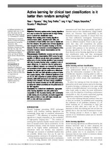
2.3. Best-versus-Second Best (BvSB) Even though EP-based active learning is often better than random selection, it has a drawback. A problem of the EP measure is that its value is heavily influenced by probability values of unimportant classes. See Figure 1 for a simple illustration. The figure shows estimated probability values for two examples on a 10-class problem. The example on the left has a smaller entropy than the one on the right.
However, from a classification perspective, the classifier is more confused about about the former since it assigns close probability values to two classes. For the example in Figure 1(b), small probability values of unimportant classes contribute to the high entropy score, even though the classifier is much more confident about the classification of the example. This problem becomes even more acute when a large number of classes are present. Although entropy is a true indicator of uncertainty of a random variable, we are interested in a more specific type of uncertainty relating only to classification amongst the most confused classes (the example is virtually guaranteed to not belong to classes having a small probability estimate). Instead of relying on the entropy score, we take a more greedy approach to account for the problem mentioned. We consider the difference between the probability values of the two classes having the highest estimated probability value as a measure of uncertainty. Since it is a comparison of the best guess and the second best guess, we refer to it as the Best-versus-Second-Best (BvSB) approach. Such a measure is a more direct way of estimating confusion about class membership from a classification standpoint. Using the BvSB measure, the example on the left in Figure 1 will be selected to query the user. As mentioned Discrete entropy = 1.69 0.5
0.4
0.45
Estimated probability
Estimated probability
Discrete entropy = 1.34 0.45
0.35 0.3 0.25 0.2 0.15 0.1 0.05 0
0.4 0.35 0.3 0.25 0.2 0.15 0.1 0.05
1 2 3 4 5 6 7 8 9 10
Class
(a)
0
1 2 3 4 5 6 7 8 9 10
Class
(b)
Figure 1. An illustration of why entropy can be a poor estimate of classification uncertainty. The plots show estimated probability distributions for two unlabeled examples in a 10 class problem. In (a), the classifier is highly confused between classes 4 and 5. In (b), the classifier is relatively more confident that the example belongs to class 4, but is assigned higher entropy. The entropy measure is influenced by probability values of unimportant classes.
previously, confidence estimates are reliable in the sense that classes assigned low probabilities are very rarely the true classes of the examples. However, this is only true if the initial training set size is large enough for good probability estimation. In our experiments, we start from as few as 2 examples for training in a 100 class problem. In such cases, initially the probability estimates are not very reliable, and random example selection gives similar results. As the number of examples in the training set grows, active learning through BvSB quickly dominates random selection by a significant margin. Note that most methods that do not use margins rely on some kind of model on the data. Therefore, probability estimation with very few examples presents a problem to most active learning methods. Overcoming this issue is an important area for future work.
2,3
1,4
1,2
1,3 3,4
Class 2
2,4
Class 3 Class 1 Class 4 2,4 3,4 1,3 2,3
1,4
1,2
Figure 2. Illustration of one-vs-one classification (classes that each classifier separates are noted). Assuming that the estimated distribution for the unlabeled example (shown as a blue circle) peaks at ‘Class 4’, the set of classifiers in contention is shown as red lines. BvSB estimates the highest uncertainty in this set – uncertainty of other classifiers is irrelevant.
2.3.1 Another perspective One way to see why active selection works is to consider the BvSB measure as a greedy approximation to entropy for estimating classification uncertainty. We describe another perspective that explains why selecting examples in this way is beneficial. The understanding crucially relies on our use of one-versus-one approach for multiclass classification. Suppose that we wish to estimate the value of a certain example for active selection. Say its true class label is l (note that this is unknown when selecting the example). We wish to find whether the example is informative, i.e., if it will modify the classification boundary of any of the classifiers, once its label is known. Since its true label is l, it can only modify the boundary of the classifiers that separate class l from the other classes. We call these classifiers as those in contention, and denote them by Cl = {C(l,i) | i = 1, . . . , k, i 6= l}, where C(i,j) indicates the binary classifier that separates class i from class j. Furthermore, in order to be informative at all, the selected example needs to modify the current boundary (be a good candidate for a new support vector – as indicated by its uncertainty). Therefore, one way to look at multiclass active selection for one-versus-one SVMs is the task of finding an example that is likely to be a support vector for one of the classifiers in contention, without knowing which classifiers are in contention. See Figure 2 for an illustration. Say that our estimated probability distribution for a certain example is denoted by p, where pi denotes the membership probability for class i. Also suppose that the distribution p has a maximum value for class h. Based on current knowledge, the most likely set of classifiers in contention is Ch . The classification confidence for the classifiers in this set is indicated by the difference in the estimated class probability values, ph − pi . This difference is an indicator of how informative the particular example is to a certain classifier. Minimizing the difference ph − pi , or equivalently, maximizing the confusion (uncertainty), we obtain the BvSB measure. This perspective shows that our intuition behind choosing the difference in the top two probability values of the estimated distribution has a valid underlying interpretation – it is a measure of uncertainty for the most likely classifier in contention. Also, the BvSB measure can then be considered to be an efficient approximation for selecting examples that are likely to be informative, in terms of changing classification boundaries.
2.3.2
Binary classification
For binary classification problems, our method reduces to selecting examples closest to the classification boundary, i.e., examples having the smallest margin. In binary problems, the BvSB measure finds the difference in class membership probability estimates between the two classes. The probabilities are estimated using Equation 1, that relies on the function value f (x) of each unlabeled example. Furthermore, the sigmoid fit is monotonic with the function value – the difference in class probability estimates is larger for examples away from the margin. Therefore, our active learning method can be considered to be a generalization of binary active learning schemes that select examples having the smallest margin.
2.4. Computational cost There are two aspects to the cost of active selection. One is the cost of training the SVM on the training set at each iteration. Second is probability estimation on the active pool, and selecting examples with the highest BvSB score. SVM training is by far the most computationally intensive component of the entire process. However, the essence of active learning is to minimize training set sizes through intelligent example selection. Therefore, it is more important to consider the cost of probability estimation and example selection on the relatively much larger active pool. The first cost comes from probability estimation in binary SVM classifiers. The estimation is efficient since it is performed using Newton’s method with backtracking line search that guarantees quadratic rate of convergence. Given class probability values for binary SVMs, multiclass probability estimates can be obtained in O(k) time per example [20], where k is the number of classes. Due to the linear relationship, the algorithm is scalable to problems having a large number of classes, unlike most previous methods. In the experiments, we also demonstrate empirical observations indicating linear time relationship with the active pool size. We were easily able to perform experiments with seed set sizes varying from 2 to 500 examples, active pool sizes of up to 10000 examples, and a up to 102-class classification problems. A typical run with seed set of 50 examples, active pool of 5000 examples, and a 10-class problem took about 22 seconds for 20 active learning rounds with 5 examples added at each round. The machine used had a 1.87 Ghz single core processor with 2 Gb of memory. All the active selection code was written in Matlab, and SVM implementation was done using LIBSVM (written in C) interfaced with Matlab. The total time includes the time taken to train the SVM, to produce binary probability values, and to estimate multiclass probability distribution for each example in the active pool at each round.
2.5. Previous work Tong and Chang [18] propose active learning for SVM in a relevance feedback framework for image retrieval. Their approach relies on the margins for unlabeled examples for binary classification. Tong et al. [19] use an active learning
method to minimize the version space1 at each iteration. However, both these approaches target binary classification. Gaussian processes (GP) have been used for object categorization by Kapoor et al. [11]. They demonstrate an active learning approach through uncertainty estimation based on GP regression, which requires O(N 3 ) computations, cubic in the number of training examples. They use one-versus-all SVM formulation for multi-class classification, and select one example per classifier at each iteration of active learning. In our work, we use the one-versus-one SVM formulation, and allow the addition of a variable number of examples at each iteration. Holub et al. [9] recently proposed a multi-class active learning method. Their methods selects examples from the active pool, whose addition to the training set minimizes the expected entropy of the system. In essence, it is an information-based approach. Note that our method computes the uncertainty through probability estimates of class membership, which is an uncertainty sampling approach. The entropy-based approach proposed in [9] requires O(k 3 N 3 ) computations, where N is the number of examples in the active pool and k is the number of classes. Qi et al. [17] demonstrate a multi-label active learning approach. Their method employs active selection along two dimensions – examples and their labels. Label correlations are exploited for selecting the examples and labels to query the user. For handling multiple image selection at each iteration, Hoi et al. [8] introduced batch mode active learning with SVMs. Since their method is targeted towards image retrieval, the primary classification task is binary; to determine whether an image belongs to the class of the query image. Active learning with uncertainty sampling has been demonstrated by Li and Sethi [12], in which they use conditional error as a metric of uncertainty, and work with binary classification. In summary, compared to previous work, our active learning method handles the multi-class case efficiently, allowing application to huge datasets with a large number of categories.
3. Experimental results This section reports experimental results of our active selection algorithm compared to random example selection. We demonstrate results on standard image datasets available from the UCI repository [1], the Caltech-101 dataset of object categories, and a dataset of 13 natural scene categories. All the results show significant improvement owing to active example selection.
3.1. Standard datasets We choose three datasets that are relevant to image classification tasks. The chosen datasets and their properties are summarized in Table 1 along with seed set, active pool, and test set sizes used in our experiments. We also report the kernel chosen for the SVM classifier. For choosing the 1 Version space is the subset consisting of all hypotheses that are consistent with the training data [14].
Dataset Pendigits USPS Letter
# classes 10 10 26
Feature dimension 16 256 16
Seed set size 100 100 100
Active pool size 5000 7000 7000
Test set size 2000 2000 5000
Kernel Linear RBF (σ = 256) RBF (σ = 16)
Table 1. Dataset properties and the corresponding sizes used. Pendigits: Pen-based Recognition of handwritten digits. USPS: Optical recognition of
94 92 90 EP BvSB Random
88 86 84 82 0
10
20
30
40
Active learning rounds
50
Examples selected per round = 5 70 60 50 EP BvSB Random
40 30 20 0
10
20
30
40
50
Active learning rounds
(a)
Classification accuracy (%)
Examples selected per round = 5 96
Classification accuracy (%)
Classification accuracy (%)
handwritten digits originally from the US Postal Service. Letter: Letter recognition dataset. All obtained from UCI [1]. Examples selected per round = 5 95 90 85 EP BvSB Random
80 75 70 0
10
20
30
40
50
Active learning rounds
(b)
(c)
Figure 3. Classification accuracy on (a) Pendigits, (b) Letter, and (c) USPS datasets. Note the improvement in accuracy obtained by BvSB approach over random selection. For similar accuracy, the active learning method requires far fewer training examples. In (b), EP-based selection performs poorly due to the larger number of classes.
kernel, we ran experiments using the linear, polynomial, and Radial Basis Function (RBF) kernels on a randomly chosen training set, and picked the kernel that gave the best classification accuracy averaging over multiple runs. Figure 3(a) shows classification results on the pendigits dataset2 . The three methods compared are EP-based selection, BvSB-based selection, and random example selection. All three methods start with the same seed set of 100 examples. At each round of active learning, we select n = 5 examples to query the user for labels. BvSB selects useful examples for learning, and gradually dominates both the other approaches. Given the same size of training data, as indicated by the same point on the x-axis, BvSB gives significantly improved classification accuracy. From another perspective, for achieving the same value of classification accuracy on the test data (same point on the y-axis), our active learning method needs far fewer training examples than random selection. The result indicates that the method selects useful examples at each iteration, so that user input can be effectively utilized on the most relevant examples. Note that EP-based selection does marginally better than random. The difference can be attributed to the fact that entropy is a somewhat indicative measure of classification uncertainty. However, as pointed out in Section 2.3, the entropy value has problems of high dependence on unlikely classes. The BvSB measure performs better by greedily focusing on the confusion in class membership between the most likely classes instead. This difference between the two active selection methods becomes more clear when we look at the results on a 26 class problem. Figure 3(b) shows classification accuracy plots on the Letter dataset, which has 26 classes. EP-based selection performs even worse on this problem due to the
larger number of classes, i.e., the entropy value is skewed due to the presence of more unlikely classes. Entropy is a bad indicator of classification uncertainty in this case, and it gives close to random performance. Even with a larger number of classes, the figure shows that BvSB-based selection outperforms random selection. After 50 rounds of active learning, the improvement in classification accuracy is about 7%, which is significant for data having 26 classes. In Figure 3(c), we show results on the USPS dataset, a dataset consisting of handwritten digits from the US Postal Service. The performance of all methods is similar to that obtained on the Pendigits dataset shown in Figure 3(a). Active selection needs far fewer training examples compared to random selection to achieve similar accuracy.
2 All results best viewed in color. All results in the paper reported by averaging over 10 runs with seed set chosen randomly at each run.
In this section, we perform experiments to quantify the reduction in the number of training examples required for
3.1.1
Reduction in training required BvSB selection rounds 3 4 5 6 7 8 9 10 11 12 13
Random selection rounds 6 10 13 19 28 29 43 44 43 48 50
% Reduction in # training examples 11.53 20 24.24 33.33 43.75 42.85 53.96 53.12 50.79 52.94 52.85
Table 2. Percentage reduction in the number of training examples provided to the active learning algorithm to achieve classification accuracy equal to or more than random example selection on the USPS dataset.
Examples selected per round = 10
accuracy between active selection and random selection starts decreasing after about 70 rounds of learning. This can be attributed to the relatively limited size of the active pool; after 70 learning rounds, about half the active pool has been exhausted. Intuitively, the larger the active pool size, the higher the benefit of using active learning, since it is more unlikely for random selection to query useful images. In real-world image classification problems, the size of the active pool is usually extremely large, often including thousands of images available on the web. Therefore, the dependence on active pool sizes is not a limitation in most cases.
3.2. Object recognition
3.3. Time dependence on pool size
3 From Figure 3(b), it seems that the reduction in training size is not as much for the Letter dataset. This is because the none of the methods have reached near-optimal performance. Experiments with more training rounds indicated that reduction was about 50% even for this dataset. 4 http://www.robots.ox.ac.uk/ vgg/research/ ˜ caltech/index.html
80
60
40 EP BvSB Random
20
0 0
20
40
60
80
100
Active learning rounds Figure 4. Active learning on the Caltech-101 dataset.
USPS dataset: seed set 100 examples
BvSB example selection time (sec)
In Figure 4, we demonstrate results on the Caltech-101 dataset of object categories [6]. As image features, we use the precomputed kernel matrices obtained from the Visual Geometry group at Oxford4 . These features give stateof-the-art performance on the Caltech dataset. The data is divided into 15 training and 15 test images per class, forming a total of 1530 images in the training and test sets each (102 classes including the ‘background’ class). We start with a seed set of only 2 images randomly selected out of the 1530 training images. We start with an extremely small seed set to simulate real-world scenarios. The remaining 1528 images in the training set form the active pool. After each round of active learning, classification accuracy values are computed on the separate test set of 1530 images. Note that in our experiments, the training set at each round of active learning is not necessarily balanced across classes, since the images are chosen by the algorithm itself. Such an experiment is closer to a realistic setting in which balanced training sets are usually not available (indeed, since providing balanced training sets needs human annotation, defeating our purpose). From Figure 4, we can see that active learning through BvSB-based selection outperforms random example selection in this 102 class problem. Interestingly, the difference in classification
Classification accuracy (%)
BvSB to obtain similar classification accuracy as random example selection. Consider a plot like Figure 3(c) above. For each round of active learning, we find the number of rounds of random selection to achieve the same classification accuracy. In other words, fixing a value on the y-axis, we measure the difference in the training set size of both methods and report the corresponding training rounds in Table 2. The table shows that active learning achieves a reduction of about 50% in the number of training examples required, i.e., it can reach near optimal performance with 50% fewer training examples. Table 2 reports results for the USPS dataset, however, similar results were obtained for the Pendigits dataset and the Letter dataset3 .The results show that even for problems having up to 26 classes, active learning achieves significant reduction in the amount of training required. An important point to note from Table 2 is that active learning does not provide a large benefit in the initial rounds. One reason for this is that all methods start with the same seed set initially. In the first few rounds, the number of examples actively selected are far fewer compared to the seed set size (100 examples). Actively selected examples thus form a small fraction of the total training examples, explaining the small difference in classification accuracy of both methods in the initial rounds. As the number of rounds increase, the importance of active selection becomes clear, explained by the reduction in the amount of training required to reach near-optimal performance.
1.5
y = 0.00018*x - 0.035 1
0.5
0 0
Actual time Linear fit
1000 2000 3000 4000 5000 6000 7000
Active pool size Figure 5. Example selection time as a function of active pool size. The relationship is linear over a large range with the equation shown in the figure. This demonstrates that the method is scalable to large active pool sizes that are common in real applications.
From another perspective, the necessity of large active pool sizes points to the importance of computational efficiency in real-world learning scenarios. In order for the methods to be practical, the learning algorithm must be able to select useful images from a huge pool in reasonable time. Empirical data reported in Figure 5 suggests that our method requires time varying linearly with active pool size. The method is therefore scalable to huge active pool sizes common in real applications.
Examples selected per round = 20
Classification accuracy
3.4. Exploring the space Exploration - seeing new classes
# classes explored
120 100 80 EP BvSB Random
60
60 50 40 30 EP BvSB Random
20 10 0 0
10
20
30
40
50
Active learning rounds % Accuracy improvement per class
40 MITstreet MIThighway
20
MITcoast MITinsidecity
0 0
20
40
60
80
CALsuburb
100
Active learning rounds
livingroom bedroom MITforest
Figure 6. Space exploration of active selection – BvSB-based selection is almost as good as random exploration, while the former achieves much higher classification accuracy than random.
MITopencountry MITtallbuilding MITmountain PARoffice kitchen
In many applications, the number of categories to be classified is extremely large, and we start with only a few labeled images. In such scenarios, active learning has to balance two often conflicting objectives – exploration and exploitation. Exploration in this context means the the ability to obtain labeled images from classes not seen before. Exploitation refers to classification accuracy on the classes seen so far. Exploitation can conflict with exploration, since in order to achieve high classification accuracy on the seen classes, more training images from those classes might be required, while sacrificing labeled images from new classes. In the results so far, we show classification accuracy on the entire test data consisting of all classes – thus good performance requires a good balance between exploration and exploitation. Here we explicitly demonstrate how the different example selection mechanisms explore the space for the Caltech-101 dataset that has 102 categories. Figure 6 shows that the BvSB measure finds newer classes almost as fast as random selection, while achieving significantly higher classification accuracy than random selection. Fast exploration of BvSB implies that learning can be started with labeled images from very few classes and the selection mechanism will soon obtain images from the unseen classes. Interestingly, EP-based selection explores the space poorly.
3.5. Scene recognition Further, we performed experiments for the application of classifying natural scene categories on the 13 scene categories dataset [5]. GIST image features [15] that provide a global representation were used. Results are shown in Figure 7. The lower figure shows accuracy improvement per class after 30 BvSB-based active learning rounds. Note that although we do not explicitly minimize redundancy amongst images, active selection leads to significant improvements even when as many as 20 images are selected at each active learning round.
-4
-2
0
2
4
6
8
10
Active selection acc. - Random selection acc.
Figure 7. Active learning on the 13 natural scene categories dataset. EPbased selection performs well possibly due to a smaller number of classes and 20 (a large number of) examples selected at each iteration.
3.6. Which examples are selected?
0
8
9
5
3
5
7
1
9
0
7
1
Figure 8. Top row shows images on which the classifier is uncertain using the BvSB score. Bottom row shows images on which the classifier is confident. True labels are noted below the corresponding images. We can see that the top row has more confusing images, indicating that the active learning method chooses harder examples.
In Figure 8, we show example images from the USPS dataset and their true labels. The top row images were confusing for the classifier (indicated by their BvSB score) and were therefore selected for active learning at a certain iteration. The bottom row shows images on which the classifier was most confident. The top row has more confusing images even for the human eye, and ones that do not represent their true label well. We noticed that the most confident images (bottom row) consisted mainly of the digits ‘1’ and ‘7’, which were clearly drawn. The results indicate that the active learning method selects hard examples for query. One of the reasons active learning algorithms perform well is the imbalanced selection of examples across classes.
# examples correctly classified
Caltech-101 dataset
is to incorporate diversity when actively selecting multiple images at each iteration, so that redundancy amongst the selected images is minimized. Notably, Holub et al. [9] can implicitly handle multiple example selection through their information-based framework. However, a big research challenge is to make such approaches computationally tractable. Another direction for future research is active learning in multi-label problems (cf. [17]), wherein each image can belong to multiple categories simultaneously.
15
10
5
0 2
4
6
8
10
12
14
# examples actively selected
Figure 9. Y-axis: # examples correctly classified by random example selection for a given class. X-axis: # examples of the corresponding class chosen by active selection. The negative correlation shows that active learning chooses more examples from harder classes.
In our case, the method chooses more examples for the classes which are hard to classify (based on how the random example selection algorithm performs on them). Figure 9 demonstrates the imbalanced example selection across different classes on the Caltech-101 dataset. On the y-axis, we plot the number of examples correctly classified by the random example selection algorithm for each class, as an indicator of hardness of the class. Note that the test set used in this case is balanced with 15 images per class. On the xaxis, we plot the number of examples selected by the active selection algorithm for the corresponding class from the active pool. The data shows a distinct negative correlation, indicating that more examples are selected from the harder classes, confirming our intuition. Notice the empty region on the bottom left of the figure, showing that active learning selected more images from all classes that were hard to classify. Next, we computed the variance in the number of examples selected per class across the 102 classes. With random selection, we expect low variance across classes owing to uniform sampling and balanced class distribution in the active pool. Random example selection gave a variance of 3.63, while active selection had a variance of 6.40. The difference in the variance reinforces our claim that the benefit to be obtained by active learning indeed relies on imbalanced selection of examples across classes. We therefore expect active learning to be particularly useful when harder classes have fewer examples so that random selection is unlikely to sample them. In real applications, it is often true that interesting images/video snippets form a rather small fraction of all the available data. We believe that active learning can be very effective in such scenarios.
4. Conclusions In this paper, we have proposed a simple active learning method for multi-class image classification. The proposed method achieves significant reduction in training required, along with efficient scaling to a large number of categories and huge data sizes. There are many interesting future work directions. One
Acknowledgment This material is based upon work supported in part by the U.S. Army Research Laboratory and the U.S. Army Research Office under contract #911NF-08-1-0463 (Proposal 55111- CI), and the National Science Foundation through Grants #CNS-0324864, #CNS-0420836, #IIP0443945, #IIP-0726109, and #CNS-0708344.
References [1] A. Asuncion and D. J. Newman. UCI machine learning repository. University of California, Irvine, School of Information and Computer Sciences, 2007. Available at http://archive.ics.uci. edu/ml/datasets.html. [2] C. Campbell, N. Cristianini, and A. J. Smola. Query learning with large margin classifiers. In ICML, 2000. [3] C.-C. Chang and C.-J. Lin. LIBSVM: a library for support vector machines, 2001. Software available at http://www.csie.ntu. edu.tw/˜cjlin/libsvm. [4] S. Dasgupta. Coarse sample complexity bounds for active learning. In NIPS. MIT Press, 2006. [5] L. Fei-Fei and P. Perona. A bayesian hierarchical model for learning natural scene categories. In CVPR, 2005. [6] L. Fei-Fei, P. Perona, and R. Fergus. One-shot learning of object categories. IEEE Trans. PAMI, 2006. [7] Y. Freund, H. S. Seung, E. Shamir, and N. Tishby. Selective sampling using the query by committee algorithm. Machine Learning, 1997. [8] S. C. Hoi, R. Jin, J. Zhu, and M. R. Lyu. Semi-supervised SVM batch mode active learning for image retrieval. In CVPR, 2008. [9] A. Holub, P. Perona, and M. Burl. Entropy-based active learning for object recognition. In CVPR, Workshop on Online Learning for Classification, 2008. [10] C.-W. Hsu and C.-J. Lin. A comparison of methods for multi-class support vector machines. IEEE Transactions on Neural Networks, 2002. [11] A. Kapoor, K. Grauman, R. Urtasun, and T. Darrell. Active learning with Gaussian Processes for object categorization. In ICCV, 2007. [12] M. Li and I. Sethi. Confidence-based active learning. IEEE Trans. PAMI, 2006. [13] H.-T. Lin, C.-J. Lin, and R. C. Weng. A note on Platt’s probabilistic outputs for support vector machines. Machine Learning, 2007. [14] T. Mitchell. Machine Learning. Boston: McGraw-Hill, 1997. [15] A. Oliva and A. Torralba. Modeling the shape of the scene: a holistic representation of the spatial envelope. IJCV, 2001. [16] J. Platt. Probabilistic outputs for support vector machines and comparison to regularized likelihood methods. In Advances in Large Margin Classifiers. MIT Press, 2000. [17] G.-J. Qi, X.-S. Hua, Y. Rui, J. Tang, and H.-J. Zhang. Twodimensional active learning for image classification. In CVPR, 2008. [18] S. Tong and E. Chang. Support vector machine active learning for image retrieval. In MULTIMEDIA ’01: Proceedings of the ninth ACM international conference on Multimedia, 2001. [19] S. Tong and D. Koller. Support vector machine active learning with applications to text classification. JMLR, 2001. [20] T.-F. Wu, C.-J. Lin, and R. C. Weng. Probability estimates for multiclass classification by pairwise coupling. JMLR, 2004.