multi-coordination methods for parallel solution of block ... - CiteSeerX

MULTI-COORDINATION METHODS FOR PARALLEL SOLUTION OF BLOCK-ANGULAR PROGRAMS By

Golbon Zakeri A thesis submitted in partial fulfillment of the requirements for the degree of

Doctor of Philosophy (Computer Sciences and Mathematics) at the

UNIVERSITY OF WISCONSIN { MADISON 1995

i

Abstract This thesis is concerned with the parallel solution of smooth block-angular programs using multiple coordinators. The research herein extends the three phase method of Schultz and Meyer, who use barrier decomposition methods with complex coordinators which are less suited to parallel computation. We start by surveying the existing literature for block-angular programs and reviewing barrier function methods and the Schultz-Meyer method. We then present our synchronous multi-coordination schemes and prove their convergence. We tested our algorithms on the Patient Distribution System problems, a class of large-scale real world multicommodity network ow problems, as well as on some randomly generated multicommodity network ow problems. Computational results on the CM-5 parallel supercomputer demonstrated that the method was signi cantly faster than its Schultz-Meyer predecessor. We also present multiple coordinator asynchronous schemes to solve block-angular programs and prove the convergence of those methods.

ii

Acknowledgements In the Name of God, the Most Gracious and the Most Merciful First and foremost I would like to thank the best thing that has ever happened to me: my husband Mark Wilson. His continuous support and witty companionship has been the most enjoyable part of my life. I would like to thank my grandmother Mrs. Esmat Sarmadi and my parents for all they have done for me throughout my life. My mother Mrs. Shahin Sabetghadam and my uncle Dr. Reza Sabet made my education possible and I am indebted to them forever. I can not imagine a better job of advising than that done by my advisor Professor Bob Meyer. He has always been the perfect advisor for me and I thank him from the depth of my heart for any success in my career. I would also like to thank my many educators from Roshangar High School, Iowa State University and University of Wisconsin. I would like to specially thank Renato De Leone and Michael Ferris for their stimulating courses and valuable discussions. Professor Frank Forelli was a great friend, teacher and mentor, may he

iii rest in peace. I thank Olvi Mangasarian and Richard Brualdi who read my thesis as well as Sigrun Andradottir and John Strikwerda for serving on my committee. Many thanks to my many friends in Madison who made life more interesting. Special thanks to my good friends, colleagues and ocemates Armand Zakarian and Geo Pritchard. I learned a great deal from our discussions. Also special thanks to Armand for the use of his software NSM. This research was partially funded by National Science Foundation grants CDA-9024618 and CCR-9306807 and Air Force Oce of Scienti c Research grant F 496 20-94-1-0036.

iv

Contents Abstract

i

Acknowledgements

ii

1 Introduction

1

1.1 Nonlinear Programming Problem : : : : : : : : : : : : : : : : : 1.2 The Block-Angular Program : : : : : : : : : : : : : : : : : : : : 1.3 A Survey of Solution Methods for Block-Angular Programs : : :

1 3 4

1.3.1 Resource Directive Decomposition : : : : : : : : : : : : : 1.3.2 Alternating Directions Method : : : : : : : : : : : : : : 1.3.3 Price Directive Decomposition : : : : : : : : : : : : : : :

4 8 9

2 A Review of Barrier Function Methods and Schultz-Meyer Decomposition 16 2.1 General Barrier Functions : : : : : : : : : : : : : : : : : : : : : 16 2.2 Convex Barrier Functions : : : : : : : : : : : : : : : : : : : : : 20 2.3 Schultz-Meyer Decomposition Scheme : : : : : : : : : : : : : : : 22

v 2.3.1 Relaxed Phase : : : : : : : : : : : : : : : : : : : : : : : : 23 2.3.2 Feasibility Phase : : : : : : : : : : : : : : : : : : : : : : 23 2.3.3 Optimality Phase : : : : : : : : : : : : : : : : : : : : : : 25 2.3.4 Schultz-Meyer Decomposition of the Barrier Problem : : 26

3 Synchronous Multi-Coordination Schemes

30

3.1 Subproblems and Decoupled Resource Allocation : : : : : : : : 32 3.2 Single-Variable Multi-Coordination : : : : : : : : : : : : : : : : 35 3.3 Group and Block-Plus-Group Multi-Coordination : : : : : : : : 40 3.4 Approximate Solution of Coordinators and Subproblems : : : : 42 3.4.1 Stabilization Algorithm for Single-Variable Coordination 42 3.4.2 Approximate Solutions for the Subproblems : : : : : : : 45

4 Computational Results

52

4.1 The Implementation : : : : : : : : : : : : : : : : : : : : : : : : 53 4.1.1 Algorithm and Implementation : : : : : : : : : : : : : : 53 4.1.2 Parameters : : : : : : : : : : : : : : : : : : : : : : : : : 54 4.1.3 The PDS Problems : : : : : : : : : : : : : : : : : : : : : 55 4.2 Analysis of the Results : : : : : : : : : : : : : : : : : : : : : : : 61 4.2.1 Single-variable multi-coordination : : : : : : : : : : : : : 61 4.2.2 Group multi-coordination : : : : : : : : : : : : : : : : : 62 4.2.3 Comparison : : : : : : : : : : : : : : : : : : : : : : : : : 63 4.3 The MNETGEN problems : : : : : : : : : : : : : : : : : : : : : 65

vi

5 Asynchronous Decomposition Methods

67

5.1 Discription of the Method : : : : : : : : : : : : : : : : : : : : : 67 5.2 Single-Variable Coordination in the Asynchronous Case : : : : : 69 5.3 Asynchronous Group Multi-Coordination : : : : : : : : : : : : : 76 5.3.1 Description of the Algorithm : : : : : : : : : : : : : : : : 76 5.3.2 Lemmas : : : : : : : : : : : : : : : : : : : : : : : : : : : 77 5.3.3 Convergence Theorem : : : : : : : : : : : : : : : : : : : 82

6 Future Directions

87

Bibliography

89

1

Chapter 1 Introduction In this chapter we start by describing the general nonlinear programming problem, then we introduce the block-angular problem and give some background information about it. We then discuss recent methods as well as classical methods that are used to solve this problem.

1.1 Nonlinear Programming Problem The problem we consider in this thesis falls under the general category of smooth (at least once continuously dierentiable) nonlinear programming and is denoted by (NLP):

minx f (x) subject to g(x)  0

h(x) = 0

2 where we have:

f : where g is the dual objective. The algorithm continues in a loop in this fashion until the termination criteria are met.

8

1.3.2 Alternating Directions Method De Leone, Meyer and Kontogiorgis in [5] use the \Alternating Directions" method to solve the BAP. They introduce for each block a vector of extra variables d~[k] that is an upper bound for D[k]x[k]; d~[k] indicates an allocation of scarce resources for block k (this is the resource directive component of their method). They de ne: 8 > < c (x ) if x[k] satis es the network constraints of block k h[k](x[k]) = > [k] [k] : +1 otherwise from which they form closed, proper, convex, extended real valued functions: 8P > < Kk=1 h[k](x[k]) if D[k]x[k]  d~[k] (8k) ~ ~ G1 (x[1];


; x[K]; d[1];


; d[K]) = > : +1 otherwise and

8 > < 0 if PKk=1 d[k] = d G2(y[1];


; y[K]; d[1];


; d[K]) = > : +1 otherwise The above yields an equivalent form for the BAP: min

G1(x[1];


; x[K]; d~[1];


; d~[K]) + G2(y[1];


; y[K]; d[1];


; d[K])

subject to

x[k] = y[k] (8k = 1;


; K ) d~[k] = d[k] (8k = 1;


; K )

x[k] ;d~[k];y[k] ;d[k]

Now in order to solve the linearly-constrained convex problem: min w;z F1(w) + F2(z ) subject to Aw + b = Bz

9 one can nd the saddle points of the augmented Lagrangian given below (multipliers p represent the price directive element of this approach).

L(w; z; p) := F1(w) + F2(z) + p(Aw + b ? Bz) + 2 jjAw + b ? Bzjj22 De Leone, Meyer and Kontogiorgis do this using the alternating directions method in a block Gauss-Seidel fashion:

wt+1 2 argminL(w; zt; pt )

(4)

zt+1 2 argminL(wt+1; z; pt)

(5)

pt+1 = rpL(wt+1 ; zt+1; pt)

(6)

They allow for dierent penalty factors [k] for each block and also let these factors vary with time. In the case of the reformulated BAP, step (4) amounts to solving a quadratic multicommodity network ow problem which is separable over blocks (hence this is done in parallel). Step (5) translates to adjusting the allocations to achieve feasibility and step (6) is updating the multipliers. They also investigate two other variants of the above scheme.

1.3.3 Price Directive Decomposition In price directed decomposition methods the coupling constraints of BAP are dealt with using some pricing mechanism. Examples of such pricing mechanisms are putting the binding constraints in the objective via Lagrangian relaxation, in the form of a barrier function or using other penalty terms.

10 In general, subproblems in the price directive decomposition scheme amount to minimization of a linear functional subject to the original block constraints. Subproblems are solved to gain search information used in the master and they provide the master with primal information. We will discuss a few price directed decomposition schemes below-the most famous of which is perhaps Dantzig-Wolfe. The last such example discussed here is barrier decomposition methods on which the work of this thesis is based.

Dantzig-Wolfe Decomposition The Dantzig-Wolfe decomposition method [3] solves the BAP when it is a linear program. Suppose the coupling constraints are put into the objective in the form of the Lagrangian relaxation: min cx ? (Dx ? d) s/t Block constraints

 min (c[1] ? D[1])x[1] +


+ (c[K] ? D[K])x[K] s/t Block constraints

If the vector  is chosen as the vector of optimal dual variables then the objective value of the above is the same as the optimal objective for the original problem. n o Let Sk = x[k]jA[k]x[k] = b[k] 0  x[k]  u[k] ; then Sk is a compact set and we have:

x[k] 2 Sk , (x[k] = k Xk k  0; ek = 1) where Xk is the matrix whose columns are the vertices of Sk . Then the original

11 BAP may be written as: min c[1]X11 +


+ c[K]XK K s/t D[1]X1 1 +


+ D[K]XK K  d k  0; ek = 1 (8k = 1; : : : ; K ) Now, at the rst iteration, for each block k the subproblem min c~[k]x[k] s/t A[k]x[k] = b[k] 0  x[k]  u[k] is solved in order to generate a single column of Xk (the cost c~ is arbitrary at this point). Subsequently the restricted master min (c[1]X~ 1)1 +


+ (c[K]X~ K )K s/t D[1]X~ 11 +


+ D[K] X~ 1K  d

  0;

ek = 1 (8k = 1; : : : ; K )

is solved where X~ k is an approximation (in iteration one this is just the one column obtained so far,) of Xk . The solution of the restricted master yields a set of duals ~i corresponding to the linear inequality constraints and duals ~k to the constraints ek = 1. After the initial iteration the subproblems take the form: min (c[k] ? ~ D[k] )xk s/t x[k] 2 Sk Now if the optimal objective to the subproblem (of the kth block) is less than ~k then a new column of Xk is generated which results in a new X~ k . If all the

12 subproblems have nonnegative optimal objectives then the current solution of the restricted master is an optimal solution for the the original BAP. For a more detailed discussion of the Dantzig-Wolfe decomposition method see [14].

Simplicial Decomposition This method originally developed by Von Hohenbalken [22] considers the problem min f (x) s/t x 2 X where X is a compact, convex, nonempty set and f is dierentiable. So in the context of BAP the set X is replaced by B = fxj Ax = b; 0  x  ug and the function f has \absorbed" the coupling constraints (e.g. in the form of a penalty function). The problem is decomposed into master and subproblem which are solved alternatively in a loop. At iteration t, rst the subproblem: min yrf (xt) y2X is solved where x0 is arbitrary and xt is the solution of the master from previous round if t > 0. For the case of X = B each subproblem is a linear programming problem decomposable over the blocks and the solution yt is an extreme point of B. Let Y = [y1jy2j : : : jyt] then the master problem is: min f (Y w)

w2W

13

(

where W = wj

Xt i=1

wi = 1; wi  0 (8i = 1; : : :t

)

and xt+1 = Y w where w is the optimal solution to the master problem. Simplicial decomposition is a decomposition method based on Caratheodory's theorem which makes this method applicable for any compact, convex, nonempty set X . A modi cation of simplicial decomposition is the restricted simplicial decomposition in which there are only a xed (predetermined) number of columns of

Y are stored. Restricted simplicial decomposition uses less memory than the ordinary simplicial decomposition.

Smoothed Exact Penalty Zenios and Pinar [18] introduce the following linear quadratic penalty function in the solution of BAP: 8 > > 0 if t  0 > < p~(; t) = >  t2 if 0  t   > > : (t ? 2 ) if t   As the parameter  # 0; p~(; t) approaches the piecewise linear penalty function 2

p~ =  max f0; tg : The linear quadratic penalty function is once continuously dierentiable (for  > 0). Zenios and Pinar use the linear quadratic penalty function to put the mutual constraints in the objective and this yields: M X p~(; yj ) (7) min  ( x ) = f ( x ) + x2X ; j =1

14 where yj = Dj x ? dj . They then solve the BAP using an iterative method. Initially a relaxed problem (the original BAP without the mutual constraints) is solved and they use the optimal solution x^ to set up y = Dx^ ? d. At the start of each iteration they approximately solve the smooth penalty problem (7). This is done using linearization via simplicial decomposition which makes the process parallelizable. Once the approximate solution of (7) is determined they adjust the penalty parameters. The steps are repeated in a loop until the termination criteria is met. Mangasarian and Chen have since developed a class of smoothing functions one of which is the smoothed exact penalty function [2].

Augmented Lagrangian Meyer and Zakarian [24] solve the BAP using an augmented Lagrangian approach. They put the binding constraints in the objective and obtain: K X ^ ? d^jj22 L(x; p) = ck (x[k]) + p(Dx ? d) + 2 jjDx k=1 where D^ , and d^ are subsets of the rows of D and d, corresponding to the current active set. The active set here refers to the constraints with positive multipliers, or ones that are satis ed at equality or the ones that are violated. The augmented Lagrangian algorithm then consists of minimizing L(x; pt) over

x subject to the linear equality and bound constraints, updating the multipliers, and updating the active set. These three steps are done in a loop until optimality is achieved. Meyer and Zakarian use nonlinear Jacobi algorithm with both simple and complex coordination for the rst step of the augmented Lagrangian

15 algorithm. This approach allows use of parallelism on the time consuming portion of the algorithm (step 1 of the augmented Lagrangian algorithm) in an ecient manner. This is an application of the parallel variable distribution method developed by Ferris and Mangasarian [6] to the augmented Lagrangian formulation of the BAP.

Barrier Function Methods We dedicate the next chapter to explanation of barrier function methods and Schultz-Meyer decomposition scheme for solution of barrier problems. The method developed here is a decomposition method related to Schultz-Meyer which uses parallel coordination. Our synchronous methods are presented in chapter 3. We present the numerical results for synchronous results in chapter 4 and asynchronous methods are discussed in chapter 5.

16

Chapter 2 A Review of Barrier Function Methods and Schultz-Meyer Decomposition In this chapter we introduce the barrier function method and review some classical results for barrier functions. We then present a compact version of the Schultz-Meyer decomposition scheme for the solution of BAP which uses barrier functions.

2.1 General Barrier Functions If the mutual constraints were not present in the formulation of BAP the constraints would be separable over the blocks (if we further had separability of the

17 objective function c(x) then the problem would be completely separable). In order to remove the coupling constraints we may place them in the objective in the form of a barrier function. Barrier functions were rst introduced by Frisch [9] and later analyzed in great detail by Fiacco and McCormick [7].

De nition 1 (Barrier function) Let  : < Jj=1 j (sj ) if s > 0 => : +1 otherwise

then  is said to be a barrier function if and only if the three properties below hold for all j = 1; : : : ; J .

 j : 0 ! < is continuous.  lim#0 j () = +1.  (80 <  <  ) j ()  j ( ), that is j is decreasing. Note that  in eect introduces a barrier that separates s > 0 from other points s 2 v. The above result on the existence of compact perturbation set is due Fiacco and McCormick (theorem 7 of [7]). We now proceed with the main theorem:

Theorem 2 Suppose that 1. c and D are continuous, 2. there exists some point z with D(z ) < d, 3. the set of local minima of the constrained problem (9) X  corresponding to the value v  = c(X  ) is a nonempty compact set, 4. X  is isolated in

Y = fyjD(y)  d and c(y) = vg 5. at least one point in X  is in the closure of fxjD(x) < dg, and 6.  i # 0 monotonically. Then 1. there exists a compact set S such that X   S  and for  i small enough the unconstrained minima of f i (:) in fxjD(x) < dg \ S  exist and every limit point of any subsequence fxig of such minimizers is in X  , 2. limi!1 c(xi) = v ,

20 3. limi!1  i(d ? D(xi )) = 0, 4. limi!1 f i (xi) = v , 5. fc(xi )g is a monotonically decreasing sequence, 6. f(d ? D(xi ))g is a monotonically increasing sequence.

2.2 Convex Barrier Functions If the functions c; D and  are convex then the function f described above would be convex. When convexity is assumed some of the assumptions for theorem (2) are unnecessary. We will assume convexity for our results. A well known and widely used barrier function is the logarithmic barrier function given by:

(d ? D(x)) = ?

J X j =1

ln(dj ? Dj: (x))

The log barrier function has the very nice property of -optimality stated below:

Theorem 3 (-optimality of Logarithmic Barrier) Suppose x is the optimal solution of the convex constrained problem (9) and x is the optimal solution of the logarithmic barrier problem formed from (9). Then

c(x)  c(x)  c(x) +  where  = :J (recall that J is the number of constraints in (9) and  is the penalty parameter).

21 Schultz in his thesis presents a proof of this theorem in conjunction with other relevant theorems. Here we present a slightly shorter proof. Proof First let us write the dual to problem (9): maximize c(x) + 0(D(x) ? d) ;x

(10)

subject to c0(x) + 0rD(x) = 0

0 Now suppose x is feasible for (9) and (^x; ^ ) is feasible for the (10) problem. Then we have: h i c(^x) + ^0(D(^x) ? d) = c(^x) + ^0(D(^x) ? d) + c0(^x) + ^0rD(^x) :(x ? x^) = [c(^x) + c0(^x)(x ? x^)] + < ^; (D(^x) ? d + rD(^x):(x ? x^)) >

 c(x) + ^0(D(x) ? d)  c(x)

(11)

The rst equality is due to feasibility of (^x; ^) for (10), and the second equality is obtained by merely rearranging the terms. The rst inequality is obtained using convexity of c and D and the fact that the gradient of a convex function underestimates it. The nal inequality is due to x feasible for (9) and ^  0. So now let x^ = x where x is the optimal solution of the log barrier problem. Also de ne ^ componentwise by:

 (^)j = d ? D j j: (x)

22 Then since x is the optimal solution of the barrier problem we have that

c0(^x) + ^0rD(^x) = 0 Hence by (11) and by de nition of ^ and x^ we get:

c(x) ? :J  c(x) So by feasibility of x for (9) and the above we obtain:

c(x)  c(x)  c(x) + 

(12)

2.3 Schultz-Meyer Decomposition Scheme Schultz and Meyer [20] use the barrier function techniques to transform the BAP to the BP. They then apply a three phase decomposition scheme to solve the BP. In order to solve the BP one needs to start with a point that satis es the mutual constraints (as well as block and bound constraints). The starting point needs to satisfy the mutual constraints strictly. To obtain such a point they go through the feasibility phase. Once a feasible point is obtained they move toward optimality while maintaining feasibility. We will now proceed with the description of the Schultz-Meyer three-phase method on which our methods are based.

23

2.3.1 Relaxed Phase The aim of this phase is to come up with an initial point. At this stage the relaxed problem:

c(x)

minimize x

subject to A[k]x[k] = b[k] k = 1; : : :; K

0xu is solved. If the objective function c(x) is separable over the blocks (which in practice is often the case) this step can be done in parallel. That is, each processor i (i = 1; : : : ; K ) would be responsible for solving the following problem:

c[i](x[i])

min xi [ ]

subject to A[i]x[i] = b[i]

0  x[i]  u[i] The optimal solution of the relaxed phase is then the concatenation of the optimal x[i]'s produced by each processor and the optimal objective the sum of the optimal objectives of the processors.

2.3.2 Feasibility Phase At the start of this phase there is a point x0 available (obtained in the relaxed phase) which satis es the block and the bound constraints. The aim here is to produce x^ which satis es the block and bound constraints and also satis es the

24 coupling constraints strictly (that is D(^x) < d). Hence if x0 happens to satisfy the coupling constraints strictly then we go on to the next phase. Otherwise the method of shifted barriers is applied to obtain x^:

De nition 3 (Shifted Barrier Problem) We will denote the following problem (SBP):

  P (; ) = min f (x; ) = c(x) + ( ? D(x)) s/t x 2 B x

(recall that B = fxj Ax = b; 0  x  ug :) Schultz and Meyer solve a sequence of (SBP) in which the shifted barrier fi g tends to the original barrier d. Let xi be the approximate minimizer of P (; i), then they choose i+1 such that the following hold:

D(xi ) < i+1  i and i+1  d

(13)

and in the limit either 1 = d or (9j ) such that limi inffji ? Dj: (xi)g = 0 (14) They show (in theorem 2.7 of [20]) that one can obtain a strictly feasible point x^ using shifted barrier methods provided the original BAP has a strictly feasible point.

Theorem 4 (Finite Feasibility) Suppose c(:) is bounded from below on B. Also let i+1 be chosen to satisfy (13) and (14). If xi 2 B are computed so that supi f (xi ; i ) is nite, then a point z 2 B \ C  exists and will be found in a nite number of steps. On the other hand if no such point exists then

f (xi; i) ! +1.

25 They propose the following algorithm for choosing i which they prove (in theorem 2.9 of [20]) satis es the conditions (13) and (14): 8 > < dj if Dj:(x0) < dj 1 j = > : Dj:(x0) +  if Dj:(x0)  dj where  > 0 is a constant. After computing xi set: 8 > < dj if Dj:(xi) < dj i j = > :  Dj:(xi) + (1 ?  )ji if Dj:(x0)  dj

(15)

(16)

The parameter  2 (0; 1) is prechosen and xed. Note here that an ecient algorithm for solving the shifted barrier problem (SBP) plays a key role in nding a feasible point.

2.3.3 Optimality Phase We reach this phase if x^ = x0 (found in the relaxed phase) satis es the coupling constraints strictly or if we've gone through the feasibility phase and have obtained a point x^ that not only satis es the network and bound constraints but also satis es the coupling constraints strictly. Schultz in his doctoral thesis refers to this stage of the algorithm as the \Re ned Phase". Here the initial point x^ is \re ned" through an iterative process and the algorithm terminates with an approximately optimal point x. Essentially the algorithm will proceed as follows:

26 Repeat until suitable xi is achieved: generate xi, the approximate solution of P ( i; d), set  i+1 = max(inf;   i)

inf and  are prechosen factors where  2 (0; 1) and inf is very small (e.g. 10?6 ). As observed from the above the major step in both feasibility and optimality phase is to approximately solve the barrier problem P . This is the central point of Schultz-Meyer decomposition algorithm and also of this thesis. We will proceed by presenting decomposition scheme and the relevant theorems, discuss the improvements relative to Schultz-Meyer and present our methods (in chapters 3{5) which incorporate these improvements.

2.3.4 Schultz-Meyer Decomposition of the Barrier Problem In order to generate an approximate solution of P (; ); Schultz and Meyer start with an initial feasible point x (e.g. x0 in the rst iteration of the feasibility phase or x^ at the start of the optimality phase). At each iteration they rst nd search directions by solving subproblems and then use this information in a coordination step to come up with a new iterate with a better objective value.

27

Convex Quadratic Subproblems At each iteration t, Schultz and Meyer use subproblems of the form: minimize y

gt(y ? xt) + (y ? xt)Gt(y ? xt)

subject to

Ay = a and 0  y  R(xt)

(17) (18)

where gt satis es: lim jjgt ? rf (xt)jj = 0

t!1

and the symmetric matrices Gt satisfy: (9 > 0) (8 t; x)

0  x0Gtx  jjxjj2

Note here that if Gt = 0 then the above quadratic subproblem turns into a linear subproblem. The subproblem presented above is the minimization of a second (or in special cases rst) order approximation of the barrier problem subject to the network and bound constraints. The upper bound R(xt) acts as a type of trust region to eliminate taking very short steps (this is small w variables or large values of y variables). We tried the algorithm without using the decoupled resource allocation and we got very poor computational results in that the convergence was much slower. Ordinarily there would be an equivalent of R(xt) for the lower bounds on the variables, however since the matrix of coupling constraints is non-negative the lower bounds remain at zero for the decoupled

28 resource allocation (see [20]). If the matrix Gt is chosen appropriately (e.g. taking Gt to be a block diagonal approximation of the hessian of f (xt) or Gt = 0) then (17) is decomposable over the blocks. Hence the subproblem can be solved in parallel.

Coordinator Problem Once the subproblem is solved and search directions y[tk] for each block k are determined then we need to determine what stepsize is to be taken in each block. Consider the search matrix at iteration t: 0 1 t t 0 CC BB y[1] ? x[1] : : : B C ... ... Yt =B 0 CCC BB @ A 0 : : : y[tK] ? xt[K] the Schultz-Meyer decomposition method nds the relevant stepsizes by approximately solving the problem below (we will denote this problem SMC). min f (xt + Y tw) subject to 0  xt + Y tw  u:

w2 t (t) < x[i] if i 6= j y[i] = > : y[tj] otherwise and denote E (j (t); t) by E (t). Now by the boundedness of resource allocation (20) we have that fy(t)g is bounded hence the sequence may further be thinned to obtain y(t) ! y~. Now for all  2 (0; 1] the following holds:

f ((1 ? )x(t) + y(t))  [xmin f (x) ? f (x(t))] 2E (t)  1 [f (x(t)+1) ? f (x(t))] (The rst inequality is due to de nition of E (t) and the second follows from (29).) Since the right hand side ! 0 as t ! 1 we have f ((1 ? )~x + y~) ? f (~x)  0. Taking the limit as  approaches 0 we get rf (~x)(~y ? x~)  0. This together with (5) proves the conclusion.

40

3.3 Group and Block-Plus-Group Multi-Coordination In this section there are two multiple coordination schemes presented as alternatives to single-variable coordinators: \group" coordinators and \block-plusgroup" coordinators. There are no changes in the subproblems. A group coordinator is used when instead of a 1 ? 1 relationship between subproblems and coordinators, each coordinator is responible for a group of subproblems. Let  f1; :::; K g denote the group of subproblems coordinator p is responsible for. Also let Y t be the matrix described columnwise below: 8 > if l 62 l < 0 t (30) (Y ) = > : (ylt ? xt) if l 2 Then the p-th coordinator problem is formed as: t t t t min w f (x + Y w) subject to 0  x + Y w  u :

Let i = i( ) 2 be the index of the subproblem that produced the best direction among those in group . Then coordinator p computes xt+1(p) = xt + Y tw that satis es: (8t) f (xt+1(p)) ? f (xt)  [x2min f (x) ? f (xt)] E (i;t)

(31)

(Note that the above is certainly satis ed at optimality since E (i; t) is a subset of the feasible region for the p-th coordinator.) The computationally checkable condition for (31) is the same as that for (28) in section 1.2. Now xt+1 is chosen among xt+1(p) 's so that f (xt+1)  f (xt+1(p)) (8p). Hence

41 if 1  j  K is the index of the subproblem that produces the best direction it follows that:

f (xt+1) ? f (xt)  [x2min f (x) ? f (xt)] E (j;t) Therefore the crucial inequality for the proof of the decomposition method using multiple coordinators (6) is preserved. This yields convergence for the group coordinator case. A \block-plus-group" coordinator handles a particular original block of variables i explicitly as well as stepsize variables for directions provided by a group of subproblems (i 62 ). A block-plus-group coordinator problem is then formed as: min ;x i

[ ]

subject to

f (x[1] + 1 (Y t)1; :::; x[i?1] + i?1 (Y t)i?1; x[i]; x[i+1] + i+1(Y t)i+1; :::; x[K] + K (Y t)K ) A[i]x[i] = b[i] 0  x[l] + l (Y t)l  u[l] (8l 2 ) 0  x[i]  u[i]

Now let ~i 2 fig[ be the index of the subproblem producing the best direction among those in or the ith subproblem. Then the block-plus-group coordinator responsible for i and ( say coordinator p) computes xt+1(p) such that: (8t) f (xt+1(p)) ? f (xt)  [ min~ f (x) ? f (xt)] x2E (i;t)

(32)

(Again E (~i; t) is a subset of the feasible set for the block-plus-group coordinator therefore (32) hold at optimality.) The computationally checkable condition for

42 (32) is the same as that for (28). Same as before, xt+1 is chosen among xt+1(p) so that f (xt+1)  f (xt+1(p))(8p). So if 1  j  K is the index of the subproblem that produces the best direction it follows that: t)] f (xt+1) ? f (xt)  [x2min f ( x ) ? f ( x E (j;t)

Therefore the convergence proof carries through for block-plus-group coordinators as well.

3.4 Approximate Solution of Coordinators and Subproblems 3.4.1 Stabilization Algorithm for Single-Variable Coordination We may use the stabilization algorithm outlined in gure 2 for approximately solving the single variable coordinator k:

Let xt+1;k = xt + tk (xt + ykt ). De ne j (t) to be the index of the block with least subproblem objective. Also de ne c(t) to be the index of the coordinator with least objective at time t. Then we choose xt+1 = xt+1;c(t), so we have

f (xt+1)  f (xt) + 1tk rf[tk]:(y[tk] ? xt[k])

(8k)

43 We now proceed to prove the convergence of stabilization algorithm:

Theorem 7 (convergence of stabilization for SVC) Suppose  f is essentially smooth and B is closed and convex,  x0 2 B is given,  the iterates xt are bounded (one way of insuring this is to assume the upprebounds u < 1),  ykt de ned as in (27),  xt+1 and t chosen according to the stabilization algorithm. Then

 The stabilization algorithm terminates in a nite number of steps,  the svc algorithm produces a sequence fxtg of feasible points,  if x~ is a limit point of fxtg then x~ is a KKT point for the barrier problem.

Proof We thin the sequence so that: xt ! x~ yjt(t) ! y~

44 1. For each coordinator k, the stabilization algorithm terminates in a nite number of steps with tk 2 [0::1]: We have

f (xt + (ykt ? xt)) ? f (xt) ? rf[tk]:(y[tk] ? xt[k]) 2 O(2 ) therefore for  small enough, the stabilization condition (33) is satis ed. We know 1  1 hence  can get as small as desired. 2.We start with x0 2 B and  2 [0::1] and ykt feasible for the coordinator, hence we maintain feasibility from xt to xt+1. 3.Here we want to prove that using stabilization algorithm, if x~ is a limit point of the sequence xt, then x~ is a KKT point for the barrier problem: Our algorithm ensures f (xt+1)  f (xt), so either f (xt) ! ?1 in which case the problem is unbounded or limt!1 f (xt+1) ? f (xt) = 0. In the latter case (33) shows: lim inf t rf t (yt ? xt[j(t)])  0 t!1 j (t) [j (t)] [j (t)] but

rf[tj(t)]:(y[tj(t)] ? xt[j(t)]) = rf t:(yjt(t) ? xt) by def of yjt(t): Hence lim inft!1 tj(t)rf t:(yjt(t) ? xt)  0. Now if tj(t) is bounded away from zero we have: lim inf rf t:(yjt(t) ? xt)  0 t!1 and the theorem is proved using suciency of search directions lemma. So consider tj(t) for which a subsequence j((t)(t)) ! 0 ( we'll drop the subscript 

45 from here on). Let f (xt+1;k ) be the objective of the kth coordinator at time t + 1, then from the stabilization algorithm and the fact that tj(t) ! 0 we have: tj(t) t t f (x + (yj(t) ? xt)) > f (xt) +

1 tj(t)rf t(yjt(t) ? xt) 2 2 t

( otherwise we would have terminated with  =  j t .) Hence ( ) 2

f (xt +

tj(t)

2

Since tj(t) ! 0 we get:

(yjt(t) ? xt)) ? f (xt) 1 t t > rf :(yj(t) ? xt) tj(t) 2

rf (~x):(~y ? x~)  1rf (~x):(~y ? x~) So we have rf (~x):(~y ? x~)  0 and hence the claim is proved.

3.4.2 Approximate Solutions for the Subproblems Here we present two theorems which establish convergence of the single-variable decomposition method when subproblems are only approximately solved.

Theorem 8 Assume we solve the subproblems such that the optimality gap is less than  i at each iteration i, and that f t g ! 0: Also assume:  fxtg  B \ dom f;  xt ! x~ 2 B \ dom f;  yt are the search directions found from subproblems and yt = yjt(t) is as in (27),

46

 there exists y~ 2 lim ptfytg with rf (~x)(~y ? x~)  0

(34)

are satis ed. Then we will prove that

8z 2 B rf (~x)(z ? x~)  0:

Proof WLOG thin the sequence so that yt ! y~: For any block l then (8 > 0) 9t > 0 such that (8t > t)

g[tl](y[tl] ? xt[l]) + (y[tl] ? xt[l])T Gt[l](y[tl] ? xt[l]) > ?:

(35)

Now suppose for some z 2 B

rf (~x)(z ? x~) = ? < 0: ~ De ne t as in the paper and Still further thin the sequence so that Gt ! G: ~ := lim inftt > 0: Then  2 (0; 1) independent of t may be picked such that:

~ (z ? x~)T G~ (z ? x~) < =2 then

~ rf (~x)(z ? x~) + 2~2(z ? x~)T G~ (z ? x~) < ? 2~ < 0:

Hence (9t~ > 0) such that (8t > t~)

gt[t(z ? xt)] + [t(z ? xt)]T Gt[t(z ? xt)] < ? 4~ < 0:

47 This implies there exists a block m such that:

~ < 0 g[tm][t(z[m] ? xt[m])] + [t(z[m] ? xt[m])]T Gt[m][t (z[m] ? xt[m])] < ?  4K where K is the number of the blocks. Let Q[m](x) represent the subproblem objective at x. Then ~ < 0 Q[m](t(z ? xt)) < ?  4K However (8t > t K ) we have ~ Q[m](y[tm] ? xt[m]) > ?  8K However t, the duality gap, is decreasing to zero. So  ~ : 9t such that (8t > t) t < 16 K So now let t > max(t~; t; t K ) then: ~ jQ[m](t(z ? xt)) ? Q[m](y[tm] ? xt[m])j >  8K But the duality gap t < 16K~ ; and this yields a contradiction. 8

~

8

~

Another termination criteria for the subproblems can be formed using a bound on the optimality gap. We rst develop a method for obtaining such bound and then use this for the subproblem termination criteria. Here we assume that the upper bounds u are nite. This works well since in practice it is often the case. (P) Minimize f (x) subject to Ax = a

0xu

(D) maximize f (x) + (Ax ? a)+ r(x ? u) + sx subject to rf (x) + A + r ? s = 0

 free, r; s  0

48 Now, for any point x that is feasible for (P) we may construct ; r and s such that (x; ; r; s) is feasible for (D) (one way of doing this is to take  = 0 and write rf (x) = s ? r with s; r  0 and hence we have a bound on the optimality gap given by:

r(u ? x) + sx: Now the objective is to nd the sharpest such bound, so we look for the optimal solution of the following: minimize

r(u ? x) + sx

(36)

subject to s ? r = rf (x) + A

s; r  0: Let g = rf (x); then (36) is equivalent to minimize (A)x + ru

(37)

subject to A + r  ?g

r0 except the optimal objectives vary by a constant ( objective of (36) is the objective of (37) plus gx). Now we write the dual to (37): (D37) max ?g , (D37') min g s/t A = a s/t A = a 0 u 0 u So the sharpest bound on the optimality gap obtained in this manner is =

?the optimal solution of (D37') + gx. Also the above demonstrates the process

49 of nding the bound on the gap is completely parallelizable and timewise equivalent to solving a subproblem. For our particular test problems however, this gap was a vast overestimate and did not work well as a convergence criteria. Now suppose that using t, the bound on the optimality gap at time t, we use the following scheme for solving subproblems approximately:

Theorem 9 Suppose the above scheme is used to generate approximate solutions for the subproblems. Also suppose:

 fxtg  B \ dom f;  xt ! x~ 2 B \ dom f;  yt are the search directions found from subproblems and yt = yjt(t) is as in (27),

 there exists y~ 2 lim ptfytg with rf (~x)(~y ? x~)  0

(39)

 The optimal objective value for barrier problem is f  2 t0):

rf[tm(t)](z[m(t)] ? xt[m(t)]) < 4?K however

rf[tm(t)](y[tm(t)] ? xt[m(t)])  4?K

So if there is a subsequence (t) for which the above subproblems had been solved to optimality then the above presents a contradiction in view of theorem 5 and we obtain the conclusions using theorem theorem 6. Hence the approximate optimality criteria of (38) must have been satis ed in the blocks m(t) for all

t > t0. Therefore: 0  f (xt) ? f   1 t  1 rf[tm(t)](xt[m(t)] ? y[tm(t)]  1 optt where optt is the optimal subproblem solution for block m(t). Now we know

optt # 0 therefore f (~x) = f  so by minimum principle optimality condition we arrive at the conclusions.

51

Given 0 < 1 < 2  3 < 1 if else

rf[tk]:(y[tk] ? xt[k])  0 set tk = 0

set  = 1 repeat until explicitly stopped : if (f (xt + (ykt ? xt))  f (xt) + 1rf[tk]:(y[tk] ? xt[k]) then tk =  and stop. else  = 2 and continue.

(33)

Figure 2: Stabilization Algorithm for Single-Variable Coordination

Terminate with the subproblem for block k if:

rf (xt)[k](y[tk] ? xt[k]) < 0 and rf (xt)[k](xt[k] ? y[tk])   t

(38)

for  2 (0; 1), or if the above is not possible terminate with the optimal LP solution. Figure 3: Approximate Optimality for Subproblems

52

Chapter 4 Computational Results In this chapter we present computational results from the implementation of single-variable and group multi-coordination schemes. We start by describing the test problems and sketch a compact version of our solution algorithm. We will then present the values of the parameters in our code. In the last section of this chapter we present our computational results for each of the above mentioned schemes and compare them to those of De Leone [14], Zenios and Pinar [18], McBride and Mamer [15], Schultz and Meyer [20] and Grigoriadis and Khachiyan [10].

53

4.1 The Implementation 4.1.1 Algorithm and Implementation As we discussed in chapter 2, our algorithm follows the basic three phase method of Schultz and Meyer. Figure (4) presents a sketch of the three phase method. Although we use the same structure as the three phase method, we generate approximate solutions of the shifted barrier problem using single-variable or group multi-coordination schemes. The algorithm for approximately solving (SBP) using single-variable multi-coordination is presented in (5) and the group multi-coordination scheme is presented in gure (6). We implemented our code on the Thinking Machines Corporation's Connection Machine CM-5. The machine runs the CMOST 7.3 operating system and we used the CMMD message passing library for inter-processor communication. In the single-variable coordination scheme very little inter-processor communication is necessary since each processor uses only the search direction it produced to solve the sv-coordinator problem. In fact the only inter-processor communication in this algorithm takes place when we look for the candidate with the least coordinator objective (see step 3 of (5)). This is done using the reduce command which very eciently searches all processors for a minimum such value. The group coordination scheme calls for more communication. Each processor, prior to solving its assigned coordinator problem needs to know the search

54 directions for the blocks in its group. We could have used the scan command available from the CMMD library so that each node would only get the information regarding the group assigned to it. However we found the concat command more exible and ecient. Had we used the scan command, there would be j j ? 1 passes (where is the group) through the processors to distribute the necessary information. We used concat to allow every processor to have information about the current search direction on every node (the entire vector y rather than y[k] for some blocks k). The algorithm would terminate if the maximum subproblem objective norm was less than the parameter spobj-tol or passed a certain number of iterations. We ran the code until we achieved at least six digits of accuracy in the optimal objective (compared with the previous results obtained by Schultz and Meyer).

4.1.2 Parameters In all instances we used the log barrier function to form the barrier problem. We also scaled the cost coecients so that jjcjj1 = 1. The rest of the parameters were as follows:

  = 10?2 is the original amount of perturbation for the shifted barrier.   = 0:95 is the parameter used in (16) to produce a sequence of shifted barriers which converge to the original barrier.

55

  0 = 100 is the initial value of the penalty parameter. The objective costs are scaled so that jjcjj1 = 1.  inf = 10?6 is the minimum possible value for the penalty parameter.  = 10?8 is the parameter used in determining the value of the decoupled resource allocation. This small value of allows for a close approach to the boundary of the trust region.

  = 1010 (which turns out to be a redundant upper bound for decoupled resource allocation of our test problems).

 ! 2 (0:5; 0:9) worked well. ! is the scaling factor used in determining the decoupled resource allocation.

 fact 2 (0:25; 0:4) the factor by which we dropped the penalty parameter (for the larger problems we used a greater value of fact which corresponds to a more gradual decrease of the penalty parameter).

4.1.3 The PDS Problems The class of test problems is referred to as the Patient Distribution System (or PDS) problems. We chose the PDS problems to test our algorithm because these are real world problems and quite a few recently developed methods (including the Schultz-Meyer) have used PDS problems as bench mark. The PDS model is a logistics model designed to help make decisions about patient evacuation.

56

Assume that the parameters  > 0  2 (0; 1)  1 > 0 inf > 0  2 (0; 1) are given. Also recall:

B = fxj Ax = b; 0  x  ug C = fxj Dx  dg RELAXED PHASE

i=0 Compute x0 as the solution of the \relaxed" problem If we determine that B = ; then quit Set 1 as in (15) If x0 2 C  Then go to the re ne phase Otherwise go to the feasibility phase

FEASIBILITY PHASE

i = i+1 Generate xi as an approximate solution of P ( i; i ) Set i+1 as in (16)  i+1 =  i If xi 2 B \ C  Then go to the re ne phase Otherwise repeat the feasibility phase REFINE PHASE i = i + 1 Set i = d Generate xi as an approximate solution of P ( i; i )  i+1 = max(inf;   i) Repeat the re ne phase until xi is \suitable" Figure 4: The three-phase method

57

To generate an approximate solution of P (; ) using single-variable multicoordination: 1. Solve the linear subproblem: t t min y k rf (x )[k] (y[k] ? x[k]) such that A[k]y[k] = b[k] 0  y[k]  R(xt)[k] [ ]

for each block k 2. Solve the single-variable coordinator problem: and set nator.

min f (xt + (ykt ? xt)wk ) subject to 0  xt + (ykt ? xt)wk  u wk 2< xt;k = xt + (ykt ? xt)wk where wk is the optimal solution of the

coordi-

3. Choose xt+1 = xt;c(t) where c(t) is the index of the block that produces the least objective for the barrier problem. Figure 5: Inner iteration for single-variable multi-coordination

58

To generate an approximate solution of P (; ) using group multi-coordination: 1. Solve the linear subproblem: t t min y k rf (x )[k] (y[k] ? x[k]) such that A[k]y[k] = b[k] 0  y[k]  R(xt)[k] [ ]

for each block k 2. Let k be the group of blocks node k is responsible for. We will drop the k subscript for ease of notation. Each group coordinator problem is of the form: t t t t min w f (x + Y w) subject to 0  x + Y w  u : where is the group of subproblems coordinator k is responsible for and Y t is as in (30). Set xt;k = xt + Y tw where w is the optimal solution of above.

3. Choose xt+1 = xt;c(t) where c(t) is the index of the block that produces the least objective for the barrier problem. Figure 6: Inner iteration for group multi-coordination

59 PDS-x denotes the problem that models a scenario lasting x days. Table (7) lists the sizes of the problems we considered and the reader can observe that the size of PDS-x grows rapidly as x grows. PDS problems are linear multicommodity network ow problems with 11 commodities. The column labeled max node gives the maximum number of nodes and the column labeled max arc presents the maximum number of arcs. The last two columns in the table

present the size of the problem when considered as an LP. The column labeled total constr. contains the total number of node constraints plus the number of

mutual constraints. The column labeled total var. contains the total number of arcs. The block constraint matrices for these block-angular problems are node-arc incidence matrices. We take advantage of this fact in our code and use a very ecient network ow solver NSM [23] to solve the subproblems. NSM uses the network simplex method to solve the subproblems. Since the upper bounds on the subproblems are changed from each iteration to the next (we adjust the decoupled resource allocation) we can not use \hot starting". That is, we need to start with an all-arti cial basis at every iteration. We used the optimization package MINOS [17] in the form of a subroutine (MINOS 5.4) in order to solve the coordinator problems for both single-variable and group coordination. MINOS solves the above using a reduced-gradient algorithm in conjunction with a quasi-Newton algorithm. MINOS requires any domain constraint for the objective function to be speci ed explicitly. Therefore

60 problem max node max arc coupling pds.1 126 339 87 pds.2 252 685 181 pds.3 390 1117 303 pds.5 686 2,149 553 pds.10 1,399 4,433 1,169 pds.20 2,857 10,116 2,447 pds.30 4,223 15,126 3,491 pds.40 5,652 20,698 4,672

total constr. total var. 1,473 3,729 2,953 7,535 4,593 12,287 8,099 23,639 16,558 48,763 33,874 105,728 49,944 154,998 66,844 212,859

Figure 7: Sizes of the PDS problems tested we had to put in linear constraints that imposed lower bounds on the arguments of each log term involved in the barrier function. This procedure amounted to imposing upper and lower bounds on w when using single-variable multicoordination. In the group multi-coordination case however we ended up with

J (recall J is the number of coupling constraints) linear constraints for each coordinator problem which is quite signi cant for large problems. We used the default parameters except for the feasibility and optimality tolerance which were set to 10?11 in the single-variable case and to 10?6 in the group case. We stopped at pds-40 mainly because the particular network solver we used does not work very eciently for problems larger than those in pds-40. We also tested our code on another group of problems generated by MNETGEN [1] which is a derivative of NETGEN [13] discussed later in this section.

61

4.2 Analysis of the Results 4.2.1 Single-variable multi-coordination In table (8) we present the solution results of the PDS problems we tested using single-variable multi-coordination method. In table (8) the rst column, labeled feas, contains the number of outer iterations for the feasibility phase (there were 2 inner iterations per outer iteration). During the feasibility phase, from one outer iteration to the next the variable  was changed as in (16). The next column contains the number of additional outer iterations to optimality. We changed the value of the penalty parameter  by the relation

 i+1 = min(fact   i; inf). This column is followed by the inner column which contains the number of inner iterations per outer iteration in the optimality phase. Next is the column labeled sub time. Here we summed the time it took to solve the subproblems that took longest to solve in each iteration over the number of iterations. Column coor time contains the sum of the times it took to solve the coordinators that took longest to be solved. rlx time is the time it took to solve the most time consuming subproblem in the relaxed phase. The column labeled total contains the total time taken to solve the corresponding PDS problem and comm. is the percentage of time spent on communication. The communication percentage is calculated by taking the time it took to solve the relaxed problem plus subproblem and coordination time away from the total time and then dividing this by the total time and multiplying the result by 100.

62 problem feas opt inner pds.1 5 15 2 pds.2 5 15 2 pds.3 5 18 2 pds.5 5 23 2 pds.10 5 23 2 pds.20 5 23 2 pds.30 5 20 4 pds.40 5 20 4

rlx time coor time sub time total 0.02 0.77 0.63 2.4 0.04 0.90 1.49 3.7 0.07 1.68 3.15 7.1 0.23 3.19 9.14 16.9 0.65 6.13 28.61 45.11 4.6 12.56 191.91 252.84 13.09 33.65 754.36 901.72 36.57 45.75 1404.14 1806.44

% comm. * * * * 20 17 11 17

Figure 8: Solution using single-variable multi-coordination We used asterisks to indicate the times were too small to extract a meaningful communications percentage.

4.2.2 Group multi-coordination Table (9) contains information about the solution of large PDS problems using group multi-coordination scheme. We also tried the group multi-coordination method on small PDS problems. The results for the small problems were not competitive with those found in the single- variable implementation. In table (9) the columns are labeled much the same as columns in table (8). The only new column is group size. This column contains the number of variables that we picked as the group size for each problem for the optimality phase. In the group multi-coordination, the feasibility phase was still implemented using single-variable coordinators. As shown in table (8) a feasible point was obtained very eciently using single-variable coordinators. Table (9) shows that

63 problem sub time coor time pds.10 29 6 pds.10 20 43 pds.20 192 13 pds.20 141 135 pds.30 754 34 pds.30 447 182 pds.30 308 191 pds.30 484 647 pds.30 569 647 pds.40 1404 46 pds.40 1124 189 pds.40 897 199 pds.40 1009 666 pds.40 1254 926

total group size 45 1 102 3 253 1 355 3 902 1 800 3 654 5 1273 7 1395 11 1806 1 1704 3 1434 5 1980 7 2370 11

% communication 20 37 17 21 11 20 22 11 12 17 21 21 14 7

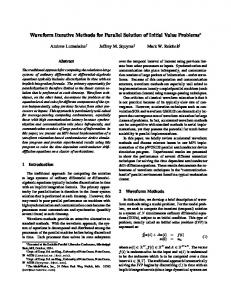
Figure 9: Comparison of single-variable and group multi-coordination for problems smaller than pds-30, solving subproblems is inexpensive and we don't gain anything from group multi-coordination. However for the larger PDS problems (e.g. PDS-30 and PDS-40) we can save time (26-27% speed up) if we choose the appropriate group size. Graph (10) plots the solution time for the large PDS problems using single-variable multi-coordination versus using group multi-coordination.

4.2.3 Comparison In table (11) we compare the best of our results with other reported results on the same set of problems. We have reviewed the methods in chapter 1. The

64 2000 1800 1600 1400 1200 1000 800 600 400 200 0

Solution Time

10

15

\single-variable" \group-coordination"

20

25

30

Problem Size 35 40

Figure 10: Single-variable multi-coordination vs. group multi-coordination rst column gives the timing results obtained by Shultz and Meyer. They implemented their method on the Sequent Symmetry machine on which each node is 5-10 times slower than the nodes of the connection machine CM5. Results obtained by Zenios and Pinar (in column labeled ZP) have been implemented on the Cray-YMP with 8 processors using the vector units hence the processors are 2-4 times faster than the nodes of CM5. Grigoriadis and Khachiyan [10] implemented their algorithm on the IBM RS 6000-550 which is 3 times faster than a node on the CM-5. McBride and Mamer [15] implemented their algorithm on the HP-730 work station which is also three times as fast as a node of the CM5. Another refrence for solution of the PDS problems (only up to pds.10) is [21].

65 problem SM ZP GK pds.10 1711 408 123 pds.20 7920 1947 372 pds.30 19380 7504 756 pds.40 37620 { 1448

MM 40 427 838 4517

MC 45 253 654 1434

Figure 11: Time comparison with other solution methods

4.3 The MNETGEN problems Another set of problems we considered were those produced by MNETGEN. We discovered that the problems produced by this generator contain some mutual constraints that held as equations for any feasible point. Therefore there is no interior for the mutual constraints. Hence we perturbed the right hand side of the mutual constraints by 1 (this perturbation is 0.06-0.25 % of the original right hand side). We anticipated diculties with these problems due to their random nature and initial lack of interior. The nal solutions obtained were ran to a sucient number of iterations (shown as col \opt") to achieve an accuracy of 4 digits (in comparison with previous results) and the timing results are reasonable. Table 12 contains the sizes and table 13 presents the results of the MNETGEN problems.

66

problem max node # blocks max arc coupling total constr. total var. 100.4 100 4 218 129 529 872 100.8 100 8 229 131 931 1048 200.4 200 4 423 252 1052 1692 200.8 200 8 449 277 1077 3592

Figure 12: Sizes of MNETGEN problems

problem # coor 100.4 1 100.4 3 100.8 1 100.8 3 100.8 5 100.8 7 200.4 1 200.4 3 200.8 1 200.8 3 200.8 5 200.8 7

opt sub time coor time 30 6.3 8.9 30 6.3 16.2 30 6.7 9.1 30 6.7 15.5 30 6.8 26.7 30 6.7 33.1 40 11.0 20.9 40 11.0 40.5 40 16.2 24.0 40 16.3 56.0 40 16.3 80.6 40 16.3 110.0

nal objective 0.668846e+06 0.668836e+06 0.131111e+07 0.131105e+07 0.131107e+07 0.131107e+07 0.164367+07 0.164154+07 0.320105+07 0.319489+07 0.319471+07 0.319413+07

Figure 13: Results for MNETGEN problems

67

Chapter 5 Asynchronous Decomposition Methods Consider the case when the number of blocks in the BAP is larger then the number of processors available. This chapter is devoted to asynchronous solution methods, one application of which is when K > P where K is the number of blocks and P is the number of available processors. We de ne a cycle length

n = dK=P e: In this chapter we require the upper bounds u on the variable x to be nite.

5.1 Discription of the Method We assume that K > P; and that information available on some blocks at time t is from previous iterations. This information has to be \recent" enough in

68 order to prove convergence. To formalize the above idea we use the \culling function" introduced by Schultz and Meyer.

De nition 4 The function  : f1; : : :; K g Z+ ! Z is called a culling function if y[k(]k;t) is a search direction used for block k at time t and (8k) tlim jjxt ? x[k(]k;t)jj = 0: !1 [k]

(40)

(For a more detailed discussion of the above de nition see Schultz's thesis [20]). We now construct a particular culling function for our algorithm. We divide the blocks into n disjoint groups, n ? 1 of which contain P blocks, while the last group contains the remaining blocks. At each iteration we concern ourselves with only one group. Hence at each iteration we have at least as many processors available as the number of blocks. Let us denote the group we process at iteration t by gt. Then at iteration t we solve subproblems for every block in group gt to obtain search directions for those blocks. We then solve single variable coordinators and choose the coordinator with the least objective value for producing the next iterate. Let k be the index of a given block and de ne 8 > =P e c ow : b t?d(k+1) n then the corresponding culling function for our asynchronous algorithm is:

(k; t) = d k P+ 1 e + n:i

(41)

69 Notice that: therefore so

t ? d(k + 1)=P e ? b t ? d k+1 P ec  1 n n k+1 t ? d k P+ 1 e ? n:b t ? dn P e c  n

t ? (k; t)  n:

5.2 Single-Variable Coordination in the Asynchronous Case In this case, at each time t a batch of blocks (P of them) gets processed in the same manner as in the synchronous case. That is, each processor produces search directions for the block it is responsible for (at time t) and proceeds to solve the corresponding single variable coordinator. Then the next iterate is taken to be the one that produced the least coordinator objective (among the blocks considered at time t) concatenated by zeros in every other block. De ne the following stabilization algorithm for solving coordinator k: Let xt+1;k = xt + tk (xt + y(k;t);k ). De ne j (t) to be the index of the block with the least subproblem objective ( here we are using the (k; t) update for each block k.) Also de ne c(t) to be the index of the coordinator with the least objective at time t. Then we choose xt+1 = xt+1;c(t), so we have

f (xt+1)  f (xt) + 1tk rf[tk]:(y[k(]k;t) ? xt[k])

(8k)

70 Given 0 < 1 < 2 < 1 if else

rf[tk]:(y[k(]k;t) ? xt[k])  0 set tk = 0

set  = 1 repeat until explicitly stopped : if (f (xt + (y(k;t);k ? xt)) ? f (xt)  1rf[tk]:(y[k(]k;t) ? xt[k]) ? jj(y[k(]k;t) ? xt[k])jj2() then tk =  and stop. else  = 2 and continue.

Figure 14: Stabilization Algorithm for Asynchronous Single-Variable Coordination The following lemma due to Schultz indicates that so long as jjxt[k] ? x[k(]k;t)jj ! 0, the \old information" y[k(]k;t) may play the role of \new information" computed relative to xt[k].

Lemma 5 Suppose that  is a culling function as described above and that yt solves the subproblems in (22) with base point xt and Gt block diagonal (blocks corresponding to the original blocks) i.e. no coupling between the subproblems. Then for t suciently large the subproblem solutions with kth block given by

y[k(]k;t) solve subproblems of the form (22). The proof for the above lemma is presented in Schultz's thesis [20]. Schultz also presents in his thesis two conditions that imply (40):

Proposition 6 Each of the following implies (40):

71 1. fxtg converges and (8k) limt!1 (k; t) = +1 2. limt!1 jjxt+1 ? xtjj = 0 and (9T ) (8(k; t)) t ? (k; t)  T

The proof for the above is very short and simple, it may also be found in [20].

Lemma 7 The stepsize t = 0 if and only if j(t) = 0: Proof Suppose j(t) = 0: This only happens if rf[tj(t)]:(y[j((jt()]t);t) ? xt[j(t)])  0: So by de nition of j (t) we have:

rf[tk]:(y[k(]k;t) ? xt[k])  0

(8k)

hence t = 0: On the other hand if t = 0 then

f (xt+1) = f (xt)  f (xt+1;j(t))

 f (xt) + j(t): 1[rf[tj(t)]:(y[j((jt()]t);t) ? xt[j(t)]) ? 2

j(t)k(y[j((jt()]t);t) ? xt[j(t)])k ] If j(t) > 0; then the right hand side is less than f (xt) and this yields a contradiction. We now proceed to prove the convergence of stabilization algorithm for the asynchronous case:

72

Theorem 10 Suppose that 1. f is essentially smooth, B is closed and convex (and we assume the upper bonds u are nite so that B is bounded), 2. we start with x0 2 B, an initial feasible point, 3. y[k(]k;t) is the search direction for block k at time t using the culling function

 from above, 4. the stepsizes t and the iterates xt are chosen according to the algorithm outlined in gure 14. Then: 1. the stabilization algorithm terminates in a nite number of steps with tk 2

[0::1]; 2. the iterates xt remain feasible, 3. either f (xt ) ! ?1 or the accumulation points of the sequence fxtg are KKT points for the barrier problem.

Proof 1. For each coordinator k, the stabilization algorithm terminates in a nite number of steps with tk 2 [0::1]: We have

k(xt[k] ? y[k(]k;t))k + f (xt + (y(k;t);k ? xt)) ? f (xt) ? rf[tk]:(y[k(]k;t) ? xt[k]) 2 O(2 )

73 therefore since 1 < 1 the stabilization condition () is satis ed for  small enough. 2.We start with x0 2 B and  2 [0::1] and y(k;t);k feasible, hence we maintain feasibility from xt to xt+1. 3.Our algorithm ensures f (xt+1)  f (xt), so either f (xt) ! ?1 in which case the problem is unbounded or limt!1 f (xt+1) ? f (xt) = 0. From here on we assume that the latter is the case. If we have a subsequence of (t) = 0 (and we will drop the ,) then :

kxt+1 ? xtk = 0 Therefore by proposition 6 we obtain property (40) and then using lemma 5 we observe that there are no descent directions left hence the theorem is proved for the subsequence with t = 0: So now we consider the case where t > 0: Using the above lemma observe that t > 0 , j(t) > 0: From the stabilization algorithm we have:

f (xt+1) ? f (xt)  f (xt+1;j(t)) ? f (xt)

 1j(t)rf[tj(t)]:(y[j((jt()]t);t) ? xt[j(t)]) ? kj(t)(y[j((jt()]t);t) ? xt[j(t)])k2 which implies: 0 < 1 

f (xt+1) ? f (xt) 2 j(t)rf[tj(t)]:(y[j((jt()]t);t) ? xt[j(t)]) ? kj(t)(y[j((jt()]t);t) ? xt[j(t)])k

Now the numerator ! 0 hence we must have the denominator approaching zero as well. The denominator consists of two negative terms hence each term has

74 to go to zero. This yields:

j(t)rf[tj(t)]:(y[j((jt()]t);t) ? xt[j(t)]) ! 0

(42)

Also if we repeat the very same argument except use t = c(t) instead of j(t) we will obtain:

kt(y[c((ct()]t);t) ? xt[c(t)])k2 ! 0

(43)

which is the same thing as:

xt+1 ? xt ! 0 4.Using proposition 6 and (43) from part 3 we conclude that  is a culling function. 5.Now suppose that x~ is a limit point of fxtg (recall that the upper bounds u were assumed to be nite). Here we will proceed to show suciency of search directions: lim inf rf[tj(t)]:(y[tj(t)] ? xt[j(t)])  0 t!1 First we consider the subsequences with j((tt)) bounded away from zero ( and again we'll drop the :) If lim inft!1 tj(t) > 0 then the stabilization algorithm together with (43) imply: lim inf rf[tj(t)]:(y[j((jt()]t);t) ? xt[j(t)])  0 t!1 and using lemma 5 we have for t large enough, y[j((jt()]t);t) = y[tj(t)]; therefore lim inf rf[tj(t)]:(y[tj(t)] ? xt[j(t)])  0 t!1

75 which combined with the suciency of search directions lemma proves the theorem. If on the other hand we have a subsequence with lim inf j((tt)) = 0 then by the stabilization algorithm we must have had:

f (xt +  j t (y[j((jt()]t);t) ? xt[j(t)])) ? f (xt) j(t) 2 >

1 [rf[tj(t)]:(y[j((jt()]t);t) ? xt[j(t)]) ?  j(t) k(y[j((jt()]t);t) ? xt[j(t)]k ] 2 2 Now further thin the sequence so that: ( ) 2

xt ! x~ and y(j(t);t);j(t) ! yt;j(t) ! y~j Then by taking limits of both sides we get: 1 rf:~ (~y ? x~)  1 rf:~ (~y ? x~): j j

2

2 Therefore since 0 < 1 < 1 and 2 > 0 we obtain

rf:~ (~yj ? x~)  0 which together with the suciency of search directions lemma proves the theorem.

76

5.3 Asynchronous Group Multi-Coordination 5.3.1 Description of the Algorithm Recall that yp(t) is the most recent search direction available for block p at time t. Here at each iteration t a dierent group of blocks is considered in the coordination step on processor p. For example if we had 12 blocks and 4 processors and we had decided that the size of coordinator 2 is two then processor number 2 would \consider" the blocks as follows: at time t = 1 the group f1; 2g at time t = 2 the group f5; 6g at time t = 3 the group f9; 10g at time t = 4 the group f1; 2g So although the set of indices of blocks involved in coordination on node p is a function of the iteration, there are only n possibilities for this (as one can observe from the example). Hence we refer to ?p;q as the group of blocks whose search direction is considered by the coordinator on node p at time t with t mod n = q. De ne Y (t) as: 0 1  (t) t 0 BB y[1] ? x[1] : : : CC B CC . ... .. (44) Y (t) = B 0 BB CC @ A 0 : : : y[K(t]) ? xt[K] Let p be the index of our processor and w^pt be the solution to the following: min

rf (xt)Y (t)w + w0H tw

77 Given 0 < 1 < 2 < 1, if rf (xt)Y (t)w^pt  0 then set tp = 0, else: Set  = 1 Repeat if f (xt + Y (t)w^pt ) ? f (xt)  1[rf (xt)Y (t)w^pt ? jjY (t)w^pt jj2] then choose tp =  and stop else reset  = 2: and continue. On processor p, the new iterate xt+1;p = xt + tpY (t)w^pt . Figure 15: Stabilization Algorithm for Asynchronous Single-Variable Coordination subject to

w[l] = 0 if l 62 ?p;q w feasible for the master problem on node p

Here we require H t to be symmetric positive de nite and have: (9 ) such that (8w) jw0H twj  jjwjj2: The following is the algorithm we propose for solving the group coordinator on processor p: Let j (t) be the index of the block with the best subproblem objective at time t and c(t) the index of the block with best (least) coordinator objective. We choose the next iterate xt+1 = xt+1;c(t) and t = tc(t).

5.3.2 Lemmas

78

Lemma 8 t = 0 if and only if tp = 0 (8p). Proof Let p be an arbitrary but xed processor index. If t = 0 then f (xt+1) = f (xt)  f (xt+1;p)  f (xt) + 1[tprf (xt)Y (t)w^pt ? jjtpY (t)w^pt jj2: So if tp > 0 then the right hand side is less than f (xt) and this yields a contradiction. Proof for the other direction is clear since t = tp for some p.

Lemma 9 If t > 0 then tj(t) > 0. Proof We will proceed by proving the contrapositive. Suppose tj(t) = 0; therefore we must have had rf (xt)Y (t)w^jt(t)  0: Hence rf (xt)Y (t)w^jt(t) + (w^jt(t))0H tw^jt(t)  0:

(45)

From (45) we will conclude rf (xt)[j(t)]:(y[j((tt))] ? xt[j(t)])  0: Assume on the contrary that rf (xt)[j(t)]:(y[j((tt))] ? xt[j(t)]) < 0, then for small enough:

rf (xt)Y (t)ej(t) + ( ej(t))0H t ej(t) < 0 where

8 > < 1 if l = j (t) (ej(t))[l] = > : 0 otherwise. Using the de nition of w^jt(t) we observe that the above contradicts (45) so we obtain: rf (xt)[j(t)]:(y[j((tt))] ? xt[j(t)])  0:

79 So, by de nition of j (t) we obtain:

rf (xt)[k]:(y[k(]t) ? xt[k])  0 (8k): This yields t = 0 which proves the lemma.

Lemma 10 Suppose (8k 2 f1::Lg) zkt  0 and we have lim inft!1 PLk=1 zkt  0, then (8k 2 f1::Lg) lim inft!1 zkt = 0. Proof Suppose that there exists r such that lim inft!1 zrt < 0. Now we know: L X k=1

zlt  zrt

(since all the terms in the sum are nonpositive). So taking lim inf of both sides we obtain: lim inf t!1 which is a contradiction.

L X k=1

zlt  lim inf zt < 0 t!1 r

Lemma 11 Suppose we have  limt!1 xt+1 ? xt = 0, and  lim inft!1 rf (xt)Y (t)w^pt  0 for a given p. Then lim inft!1 Pk2?p;q rf (xt)[k] :(y[tk] ? xt[k])  0 (8q).

Proof Using lemma 5 and proposition 6 coupled with the rst assumption we get that  is a culling function and that for t suciently large y(t) = yt. Now

80 assume on the contrary, then we thin the sequence to get: xt ! x~

yt ! y~; y(t) ! y~

rst implication is by boundedness of resource allocation,

and the second by properties of the culling function . Y t ! Y~ ; Y (t) ! Y~ by de nition of Y (t) and Y t. H t ! H~ by boundedness of eigenvalues requirement on H t. And we will have: lim inf t!1

X k2?p;q

rf (xt)[k]:(y[tk] ? xt[k]) = ? < 0

for some q. Now choose p;q 2 (0::1] so that:

X k2?p;q

~ p;q < ?p;q  p;q rf (~x)[k]:(~y[k] ? x~[k]) + 2p;q ip;q0Hi 2

where

8 > < 1 if k 2 ?p;q (ip;q)[k] = > : 0 otherwise ~ p;q ) < =2.) Since p;q 2 (0::1], p;q ip;q (Note that essentially we need p;q (ip;q 0Hi is feasible for the master on node p, so from de nition of w^pt , for t suciently large and t mod n = q we'll have:

rf (xt)Y (t)w^pt  rf (xt)Y (t)p;q ip;q + (p;q ip;q)0H t(p;q ip;q ) < ?4p;q  < 0: And this contradicts the assumption so the lemma is proved.

Lemma 12 Suppose we have  limt!1 xt+1 ? xt = 0, and

81

 lim inft!1 rf (xt)Y (t)w^jt(t)  0: Then lim inft!1 rf (xt)[j(t)]:(y[tj(t)] ? xt[j(t)])  0:

Note here that we can not merely combine lemma 11 and lemma 10 to get this since j (t) is a time dependent index. Also here we take advantage of the assumption that j (t) 2 ?j(t);q from the way we design our algorithm.

Proof Using lemma 5 and proposition 6 coupled with the rst assumption we get that  is a culling function and that for t suciently large y(t) = yt. Assume on the contrary that: lim inf rf (xt)[j(t)]:(y[tj(t)] ? xt[j(t)]) = ? < 0: t!1 Then lim inf rf (xt)[j(t)]:(y[j((tt))] ? xt[j(t)]) = ? < 0: t!1 So now de ne ij(t) blockwise by:

8 > < 1 if k = j (t) (ij(t))[k] = > : 0 otherwise

Then lim inft!1 rf (xt)Y (t)ij(t) = ? < 0. Now de ne jjHjj = lim inft!1 i0j(t)H tij(t) and choose  such that: ()(rf (xt)Y (t)ij(t)) + 2jjHjj < ?=2

82 Note here that  may be chosen independent of t so that jjHjj < =2 and this choice of  will yield the desired inequality. So then for t suciently large we have:

rf (xt)Y (t)w^jt(t)  rf (xt)Y (t)ij(t) + (ij(t))0H t(ij(t)) < ?=4: Considering  2 (0::1], observe that ij(t) is feasible for the master on node j (t) thus using the de nition of w^jt(t) we arrive at a contradiction.

5.3.3 Convergence Theorem Theorem 11 Suppose that 1. f is essentially smooth and B is closed and convex (we also include large bounds on x so that B is bounded). 2. An initial feasible point x(0) 2 B is given. 3. yp(t) is the most recent search direction available for processor p. 4. Y (t) is de ned as in (44). 5. We use the stabilization algorithm in this section to obtain new xp iterates from old ones on each processor. 6. The actual new iterate xt is the xtp which resulted in the least coordinator objective amongst all processors used in iteration t. Then

83 1. the stabilization algorithm terminates in a nite number of steps with tp 2

[0::1]. 2. For the sequence fxt g either f (xt) ! ?1 or each x~ that is a limit point of fxt g, x~ is a KKT point of the barrier problem we are minimizing.

Proof Since the feasible region is bounded we must have a limit point for the fxtg. 1. For each coordinator p the stabilization algorithm terminates in a nite number of steps with tp 2 [0::1]: For any given processor p at time t if

rf (xt)Y (t)w^pt  0 then we terminate with tp = 0 and we clearly have nite termination. If on the other hand rf (xt)Y (t)w^pt < 0 we have: f (xt+1;p) ? f (xt) ? rf (xt)Y (t)w^pt + jjY (t)w^pt jj2 2 O(2 ): Now since 0 < 1 < 1 for  small enough the stabilization condition will be satis ed hence we exit the algorithm in nite number of steps and with tp 2 [0::1]. 2. We maintain feasibility throughout the iterations since x(0) is feasible and each new iterate is a convex combination of the previous iterate and search direction both of which are feasible for the network constraints and weights are chosen so as not to violate any upper bound constraints. 3. The algorithm insures f (xt+1)  f (xt) so either f (xt) ! ?1 in which case the problem is unbounded or limt!1 f (xt+1) ? f (xt) = 0.

84 From here on we assume that the latter is the case. If we have a subsequence

(t) = 0 (and we will drop the superscript  for simplicity,) then

jjxt+1 ? xtjj = 0

(46)

tp = 0 (8p) using lemma 8.

(47)

and Therefore by (47) we must have had:

rf (xt)Y (t)w^pt  0 (8p): This together with (46) are the hypothesis of lemma 11 for any p, therefore we have the conclusion of lemma 11: X rf (xt)[k]:(y[tk] ? xt[k])  0 (8q)(8p): lim inf t!1 k2?p;q

So now we apply lemma 10 to the above to get: lim inf rf (xt)[k]:(y[tk] ? xt[k]) = 0 (8k 2 [1::K ]): t!1 Now using the suciency of search directions lemma it is clear that we have convergence for the case when a subsequence (t) = 0. So now suppose t > 0. Then from lemma 9 we get tj(t) > 0. From the stabilization algorithm we have i h f (xt+1)?f (xt)  f (xt+1;j(t))?f (xt)  1 tj(t)rf (xt)Y (t)w^jt(t) ? jjtj(t)Y (t)w^jt(t)jj2 which implies: 0 < 1 

f (xt+1) ? f (xt) : tj(t)rf (xt)Y (t)w^jt(t) ? jjtj(t)Y (t)w^jt(t)jj2

85 Now the numerator approaches 0 hence we must have the denominator approaching 0 as well. Since the denominator consists of two negative pieces we get:

tj(t)rf (xt)Y (t)w^jt(t) ! 0: And if we repeat the same argument with t instead of tj(t) then:

jjtY (t)w^jt(t)jj2 ! 0

(48)

xt+1 ? xt ! 0:

(49)

which means So using (48) and taking lim inf of both sides of the required condition of convergence in the stabilization algorithm we get: lim inf t rf (xt)Y (t)w^jt(t)  0: t!1 j (t) Now if lim inft!1 tj(t) > 0 then we have lim inf rf (xt)Y (t)w^jt(t)  0 t!1 and this together with (49) and lemma 12 proves the theorem. Now the only case remaining is lim inft!1 tj(t) = 0. Suppose tj(t)(t) is the subsequence that converges to 0. (From here on we drop the superscript ). Thus by the stabilization algorithm we must have had: t # t f (xt +  j t Y (t)w^jt(t)) ? f (xt) 1 "  2 j ( t ) > rf (xt)Y (t)w^jt(t) ? jjY (t)w^jt(t)jj : t ( ) 2

j (t)

2

2

86 Now we further thin the sequence to get:

xt ! x~; Y (t) ! Y~ ; and

w^jt(t) ! w~j : Now by taking limits from both sides of the inequality we obtain: 1 rf:~ (Y~ w~ )  1 rf:~ (Y~ w~ ): j j

2

2 Hence: lim inf rf (xt)Y (t)w^jt(t)  0: t!1 So again we use (49) and lemma 12 to establish the conclusion.

87

Chapter 6 Future Directions There are a few related areas which remain to be explored. One is the generalization of asynchronous schemes to the block-plus-group coordinators and the implementation of all asynchronous methods. The asynchronous schemes presented in chapter 5 were designed to work for the case when the number of blocks is more than the number of processors. With some minor alterations they could be used to compensate and balance loads if there is any load unbalancing present (e.g. if a block is signi cantly larger than other blocks). Here we can go through several iterations using old information for the large blocks until the corresponding subproblems on those blocks are solved and new information is obtained. Another area that needs more examination is formation of the group coordinators. As we discussed in chapter 4, we need to specify the domain constraints

88 explicitly. In the case of single-variable coordinators this translates to mere upper and lower bounds on the stepsize variable w. In the group coordinator case the logarithmic domain constraints are linear constraints. There are as many of these as the number of mutual constraints (that is a lot!) and this slows down the coordination process. Hence it is desirable to eliminate the redundant or linearly dependent constraints. Aggregation of constraints (used in bundle methods) may be a way of reducing the number of such constraints. Another approach may be to use an active set strategy. We also pointed out in the chapter for computational results that we were not able to use hot starting for solution of the subproblems. This is due to the fact that the bounds on the variable y would change from one iteration to the next since the decoupled resource allocation would change. We could update the decoupled resource allocation every few iterations rather than every iteration to achieve this. Also, the decoupled resource allocation could be designed to have more of a centering property to it. That is, making a box trust region centered around the old iterate. That way the old iterate would still be feasible as a starting solution for the subproblems.

89

Bibliography [1] Agha Iqbal Ali and J. Kennington. MNETGEN program documentation. Technical Report IEOR 77003, Department of Industrial Engineering and Operations Research, Southern Methodist University, Dallas, Texas 75275, 1977. [2] Chunhui Chen and O.L.Mangasarian. A class of smoothing functions for nonlinear and mixed complimentarity problems. Technical Report TR9411, Center for Parallel Optimization, Computer Sciences Department, University of Wisconsin, August 1994. [3] G.B. Dantzig and P. Wolfe. A decomposition principle for linear programs. Operations Research, 8:101{111, 1960.

[4] Renato DeLeone, Manlio Gaudioso, and Maria Flavia Monaco. Nonsmooth optimization methods for parallel decomposition of multicommodity ow problems. Technical Report 1080, Centre for Parallel Optimization, Computer Sciences Department, University of Wisconsin, 1992.

90 [5] Renato DeLeone, Robert R. Meyer, and Spyridon Kontogiorgis. Alternating direction splittings for block-angular parallel optimization. Technical Report 1217, Centre for Parallel Optimization, Computer Sciences Department, University of Wisconsin, 1994. [6] M.C. Ferris and O.L. Mangasarian. Parallel variable distribution. Technical Report 1175, Centre for Parallel Optimization, University of Wisconsin, Computer Sciences Dept., 1993. [7] A.V. Fiacco and G.P. McCormick. Nonlinear Programming: Sequential Unconstrained Minimization Techniques. John Wiley & Sons, New York, 1968. [8] L.R. Ford and D.R. Fulkerson. Flows in Networks. Princton University Press, Princton, NJ, 1962. [9] K.R. Frisch. The logarithmic potential method of convex programming. Unpublished manuscript, University Institute of Economics, Oslo, 1955. [10] M.D. Grigoriadis and L.G. Khachiyan. An exponential-function reduction method for block-angular convex programs. Technical Report 211, Laboratory for Computer Sciences Research, Rutgers, Computer Sciences Dept., May 1993. [11] W. Karush. Minima of functions of several variables with inequalities as side conditions. Master's thesis, University of Chicago, 1939.

91 [12] J.L. Kennington and R.V. Helgason. Algorithms for Network Programming. John Wiley and Sons, New York, 1980. [13] D. Klingman, A. Napier, and J. Stutz. NETGEN|A program for generation of large-scale (un)capacitated assignment, transportation and minimum cost network problems. Management Science, 20:814{822, 1974. [14] R. De Leone, R.R. Meyer, S. Kontogiorgis, A. Zakarian, and G. Zakeri. Coordination in coarse grained decomposition. SIAM Journal on Optimization, 4(4):777{793, 1994.

[15] Richard D. McBride and John W. Mamer. Solving multicommodity ow problems with a primal embedded network simplex algorithm. submitted. [16] Deepankar Medhi. Parallel bundle-based decomposition for large-scale structured mathematical programming problems. Annals of Operations Research, 22:101{127, 1990.

[17] B.A. Murtagh and M.A. Saunders. MINOS 5.4 release notes, appendix to MINOS 5.1 user's guide. Technical report, Stanford University, 1992. [18] M.C. Pnar and S.A. Zenios. Parallel decomposition of multicommodity network ows using a linear-quadratic penalty algorithm. ORSA Journal on Computing, 4:235{249, 1992. [19] R.T. Rockafellar. Conjugate Duality and Optimization, volume 16 of Conference Board of the Mathematical Sciences. SIAM, Philadelphia, PA, 1974.

92 [20] G.L. Schultz. Barrier Decomposition for the parallel optimization of blockangular programs. PhD thesis, University of Wisconsin-Madison, 1991.

[21] Rudy Setiono. An interior dual proximal point algorithm for linear programs. Technical Report TR879, Center for Parallel Optimization, Computer Sciences Department, University of Wisconsin, September 1989. [22] B. von Hohenbalken. Simplicial decomposition in nonlinear programming algorithms. Mathematical Programming, 13:49{68, 1977. [23] Armand Zakarian. Private communication. [24] Armand Zakarian. Parallel solution of multi-commodity network ow programs via nonlinear jacobi algorithm. Unpublished manuscript.