Cape Peninsula University of Technology
Digital Knowledge CPUT Theses & Dissertations
Theses & Dissertations
9-1-2010
Development of methods for parallel computation of the solution of the problem for optimal control Litha Mbangeni Cape Peninsula University of Technology
Follow this and additional works at: http://dk.cput.ac.za/td_cput Recommended Citation Mbangeni, Litha, "Development of methods for parallel computation of the solution of the problem for optimal control" (2010). CPUT Theses & Dissertations. Paper 323. http://dk.cput.ac.za/td_cput/323
This Text is brought to you for free and open access by the Theses & Dissertations at Digital Knowledge. It has been accepted for inclusion in CPUT Theses & Dissertations by an authorized administrator of Digital Knowledge. For more information, please contact
[email protected].
""
..
~
'i"
Cape Peninsula University of Technology
DEVELOPMENT OF METHODS FOR PARALLEL COMPUTATION OF THE SOLUTION OF THE PROBLEM FOR OPTIMAL CONTROL
by
L1THA MBANGENI
Thesis submitted in fulfilment of the requirements for the degree
Master of Technology: Electrical Engineering
in the Faculty of Engineering
at the Cape Peninsula University of Technology Supervisor: Professor, Raynitchka Tzoneva Co-Supervisor: Mr. Car! Kriger
Bellville September 2010
DECLARATION
I, Litha Mbangeni, declare that the contents of this dissertation/thesis represent my own unaided work, and that the dissertation/thesis has not previously been submitted for academic examination towards any qualification. Furthermore, it represents my own opinions and not necessarily those of the Cape Peninsula University of Technology.
Signed
Date
ii
ABSTRACT
Optimal control of fermentation processes is necessary for better behaviour of the process in order to achieve maximum production of product and biomass. The problem for optimal control is a very complex nonlinear, dynamic problem requiring long time for calculation Application of decomposition-coordinating methods for the solution of this type of problems simplifies the solution if it is implemented in a parallel way in a cluster of computers. Parallel computing can reduce tremendously the time of calculation through process of distribution and parallelization of the computation algorithm. These processes can be achieved in different ways using the characteristics of the problem for optimal control.
Problem for optimal control of a fed-batch, batch and continuous fermentation processes for production of biomass and product are formulated. The problems are based on a criterion for maximum production of biomass at the end of the fermentation process for the fed-batch process, maximum production of metabolite at the end of the fermentation for the batch fermentation process and minimum time for achieving steady state fermentor behavior for the continuous process
and on unstructured mass balance
biological models incorporating in the kinetic coefficients, the physiochemical variables considered as control inputs. An augmented functional of Lagrange is applied and its decomposition in time domain is used with a new coordinating vector. Parallel computing in a Matlab cluster is used to solve the above optimal control problems. The calculations and tasks allocation to the cluster workers are based on a shared memory architecture. Real-time control implementation of calculation algorithms using a cluster of computers allows quick and simpler solutions to the optimal control problems.
iii
ACKNOWLEDGEMENTS
I wish to thank:
•
•
• •
My parents Mandzolwandle Christopher and Fezeka Felicia Mbangeni, sister Zintle Tablsa Mbangeni, my Aunt Noxolo Mbangeni and Ntlonikazi Victoria Ketani for their support, patience endurance and understanding during the study, Professor Raynitchka Tzoneva for her invaluable help in my career. I consider myself fortunate to come across such a noble professor. She have shown a great interest in all phases of this project to ensure its success, But for her keen involvement, this thesis would not have been possible, I am thankful to her for assigning me one of the most important research project in the field of Real-Time Distributed Systems, Mr Carl Kriger for his energetic, enthusiastic on assisting with the installation of the software The Electrical Engineering Controls Group at the Cape Peninsula University of Technology for their assistance in different areas of the research,
The financial assistance of the National Research Foundation towards this research is acknowledged. Opinions expressed in this thesis and the conclusions arrived at, are those of the author, and are not necessarily to be attributed to the National Research Foundation.
iv
DEDICATION
For my Family and daughter Kanyisile Njobe
v
TABLE OF CONTENTS Declaration Abstract Acknowledgements Dedication Glossary Nomenclature
ii iii iv v xiv xv
CHAPTER ONE: INTRODUCTION 1.1 1.2 1.3 1.3.1 1.3.2 1.3.3 1.3.4 1.3.5 1.3.6 1.4 1.4.1 1.4.2 1.5 1.6 1.7 1.8 1.9 1.9.1 1.9.2 1.9.3 1.10 1.11 1.12 1.13
Awareness of the problem Statement of the problem Design based problems Sub-problem 1: Mathematical modeling Sub-problem 2: Development of decomposition methods Sup-problem 3: Software development for calculation of the on computer Sub-problem 4: Simulation of the problem Sub-problem 5: Software development for calculation of the problem on a cluster Optimization of the process of parallel computation Research Aim and objectives Research Aim Objectives Hypothesis Delimitation of Research Motivation of Research Assumption Description of the fermentation processes Fed-batch fermentation Batch fermentation Continuous fermentation Control system layers Parallel optimal control calculation Thesis outline Conclusion
1
2 3 3 3 3 3 4 4 4
4 4
5 5 5 6 6 7 7 7 8 8 9
10
CHAPTER TWO: DESCRIPTION AND PROCESS MODELING OF FERMENTATION PROCESSES
2.1
2.2 2.2.1 2.2.2 2.2.3 2.3
Introduction Fermentation process Microorganism types Fermentation process phases Comparison of fermentation processes Modeling of fermentation processes vi
11 11 11 13 14 15
2.4 2.4.1 2.4.2 2.4.3 2.5 2.6 2.6.1 2.6.2 2.6.3 2.6.3.1 2.6.3.2 2.6.4 2.6.5 2.7
Modeling Approaches White box models Black-box models Grey-box model Kinetic models Mass balance principle offermentation processes Models for Batch fermentation process Models for Fed-batch fermentation process Models for Continuous fermentation process Dynamic-state balances Steady - state equations description Physiochemical variables incorporation into the biological variables Discrete models of the fermentation processes Conclusion
16 16 16 17 17
20 22 25 28 28 30 31
32 35
CHAPTER THREE: CONTROL, OPTIMIZATION AND DECOMPOSITION OF BIOPROCESS OPTIMAL CONTROL PROBLEM
3.1 3.2 3.3 3.4 3.5 3.5.1 3.5.2 3.6 3.7
Introduction Importance of the fermentation process control Batch and fed-batch control Continuous bioprocess control Some important Adaptive Optimization Techniques Steady-State optimization Dynamic Optimization Decomposition methods for fermentation process optimal control Conclusion
36 36 40 41 41 41
42 46 48
CHAPTER FOUR: DEVELOPMENT OF A DECOMPOSITION METHOD FOR OPTIMAL CONTROL CALCULATION OF BATCH FERMENTATION PROCESS
4.1 4.2 4.3 4.3.1 4.3.2 4.3.3 4.3.4 4.4 4.6
Introduction Formulation of the problem for optimal control of a batch fermentation process Augmented Lagrange functional formulation of a batch fermentation process Necessary conditions for optimality of a batch fermentation process Coordinating vector of a batch fermentation process First level sub-problems of a batch fermentation process The coordinating sub-problem of a batch fermentation process Algorithm of the method for batch fermentation process Description of the Matlab sequential program for optimal control of batch fermentation process
vii
49 49 50 51
54 56 61 62 64
6.4 6.5 6.6 6.6.1
6.7 6.8
Algorithm of the method for continuous fermentation process Description and calculation results from the sequential program of the algorithm of the method in Matlab for continuous fermentation process Description of the Matlab sequential program for optimal control of continuous fermentation process Results from sequential calculation of continuous fermentation process Discussion of the results for continuous fermentation process Conclusion
123 126 128 129 134 134
CHAPTER SEVEN: PARALLEL COMPUTING TOOLBOX AND MATLAS DISTRIBUTED COMPUTING SERVER ON A CLUSTER
7.1 7.2 7.2.1 7.2.2 7.3 7.3.1 7.3.2 7.3.3 7.4 7.5 7.5.1 7.5.2 7.5.3 7.6 7.7 7.7.1 7.7.2 7.7.2.1 7.7.2.2 7.7.2.3 7.7.3 7.7.4 7.7.5 7.7.6 7.7.7 7.7.8 7.8 7.8.1 7.8.2 7.9
Introduction Parallel computing Amdahl's law and Gustafson's law Gustafson's law Parallel Computer Memory Architecture Shared memory Distributed memory Distributed shared memory History of Parallel MATLAB Why there should be parallel matlab Memory model Granularity Bussiness situation Parallel Matlab survey Matlab Parallel Computing Toolbox and Matlab Distributed Computing Server Parallel Computing Toolbox Terminology Programming parallel applications in Matlab Multithreaded parallelism Distributed computing Explicit parallelism Working in an interactive parallel environment Working in Batch Environments Cluster Using MATLAB Distributed Computing Server Steps in running a distributed job using Parallel Computing Toolbox (pCT) Code execution at the client and workers Design of Load balancing Algorithm Program Development Sequential in one computer Parallel, using the cluster of computers Conclusion
ix
135 135 136 136 136 136 137 137 138 139 139 140 140 140 142 143 143 144 144 144 144 145 145 146
146 147 148 148 149 151
CHAPTER EIGHT: DESCRIPTION OF THE MATLAB PARALLEL PROGRAMS FOR OPTIMAL CONTROL PROBLEM OF FERMENTATION PROCESSES
8.1 8.2 8.2.1 8.2.2 8.2.3 8.3 8.3.1 8.3.2 8.3.3 8.4 8.4.1 8.4.2 8.4.3 8.5 8.5.1 8.5.2 8.5.3 8.7
Introduction Matlab parallel program for optimal control of batch fermentation process Starting parallel computation for batch fermentation process Function for parallel calculation of batch fermentation process Results from calculations with the Matlab parallel program of batch fermentation process Matlab parallel program for optimal control of fed-batch fermentation process Starting parallel computation of fed-batch fermentation process Function for parallel calculation of fed-batch fermentation process Results from calculations with the Matlab parallel program for fed-batch fermentation process Matlab parallel program for optimal control calculation of continuous fermentation process Starting parallel computation of continuous fermentation process Function for parallel calculation of continuous fermentation process Results from calculations with the Matlab parallel program of continuous process Comparison of the results from the sequential and parallel computing of optimal state and control trajectories Comparison of the results from the sequential and parallel computing of batch fermentation process Comparison ofthe results from the sequential and parallel computing of fed-batch fermentation process Comparison of the results from the sequential and parallel computing of continuous fermentation process Conclusion
152 152 152 153 154 158 158 159 160
165 165 166 167 172
172 172 172
172
CHAPTER NINE: CONCLUSION AND FUTURE RECOMMENDATIONS
9.1 9.2 9.3 9.3.1 9.3.2 9.3.3 9.3.4 9.4 9.5
Introduction Aims and objectives Deliverables Development of the mass balance models for different types of fermentation processes Development of a decomposition method for solution of the optimal control problem Development of the algorithms and programs in Matlab for sequential calculation of the optimal control trajectories Development of the algorithms and programs in Matlab for distributed-parallel calculation of the optimal control trajectories Application of results Future research
x
173 173 174
174 174 174
175 176 176
9.6
Publications
176
BIBLIOGRAPHY
177
LIST OF FIGURES Figure 1.1: Three layers of control system Figure 2.1: General Classification of microorganisms Figure 2.2: Growth curve of a bacterial culture Figure 2.3: Typical industrial fermentation Figure 2.4: Kinetic model structure Figure 3.1: Adaptive closed-loop controls Figure 4.1: Two level calculation structure for batch fermentation process Figure 4.2: Flow chart of the algorithm for calculation of batch fermentation process state and control trajectories. Figure 4.3: Initial trajectories of state variables for batch Fermentation process Figure 4.4: Optimal trajectory of biomass for batch fermentation process Figure 4.5: Optimal trajectory of product for batch fermentation process Figure 4.6: Optimal trajectory of substrate for batch fermentation process Figure 4.7: Optimal trajectories of conjugate variables for batch fermentation process Figure 4.8: Optimal trajectory of temperature for batch fermentation process Figure 5.1: Flow chart of the algorithm for calculation of optimal trajectories of fed-batch fermentation process Figure 5.2: Initial trajectories of state variables for fed-batch fermentation process Figure 5.3: Optimal trajectory of biomass for fed-batch fermentation process Figure 5.4: Optimal trajectory of product for fed-batch fermentation process Figure 5.5: Optimal trajectory of substrate for fed-batch fermentation process Figure 5.6: Optimal trajectories of volume for fed-batch fermentation process Figure 5.7: Optimal trajectory of temperature for fed-batch fermentation process Figure 5.8: Optimal trajectory of input-flow rate for fed-batch fermentation process Figure 5.9: Optimal trajectories of conjugate variables for fed-batch fermentation process Figure 6.1: Two Level computing structure for minimum startup time Figure 6.2: Flow chart of the algorithm for calculation of continuous fermentation process Figure 6.3: Initial trajectories of state variables for continuous fermentation process Figure 6.4: Optimal trajectory of biomass for continuous fermentation process xi
8 12 14 14 18 41 56 66 71 71 72 72 73 73 94 100 100 101 101 102 102 103 103 115 125 130 130
Figure 6.5: Optimal trajectory of product for continuous fermentation process Figure 6.6: Optimal trajectories of substrate for continuous fermentation process Figure 6.7: Optimal trajectory of temperature for continuous fermentation process Figure 6.8: Optimal trajectories of Dilution rate for continuous fermentation process Figure 6.9: Optimal trajectories of conjugate variables for continuous fermentation process Figure 6.10: Optimal trajectories of state variables for continuous fermentation process Figure 7.1: Shared memory multiprocessor Figure 7.2: Distributed memory multi-processor Figure 7.3: Distributed shared-memory Figure 7.4: Typical parallel computing cluster Figure 7.5: Client, jobmanager and worker interaction Figure 7.6: Code execution Figure 7.7A: Flow chart for load balancing processing by each processor i (Pi) on every status exchange Figure 7.78: Flow chart for load balancing Processing by Pi on arrival of job j Figure 7.8: Sequential programming block diagram Figure 7.9: Parallel programming block diagram Figure 8.1: Initial trajectories of state variables for batch Fermentation process Figure 8.2: Optimal trajectory of biomass for batch fermentation process Figure 8.3: Optimal trajectory of product for batch fermentation process Figure 8.4: Optimal trajectory of substrate for batch fermentation process Figure 8.5: Optimal trajectories of conjugate variables for batch fermentation process Figure 8.6: Optimal trajectory oftemperature for batch fermentation process Figure 8.7: Initial trajectory of state variables for fed-batch fermentation process Figure 8.8: Optimal trajectory of biomass for fed-batch fermentation process Figure 8.9: Optimal trajectory of product for fed-batch fermentation process Figure 8.10: Optimal trajectory of substrate for fed-batch fermentation process Figure 8.11: Optimal trajectory of volume for fed-batch fermentation process Figure 8.12: Optimal trajectory of temperature for fed-batch fermentation process Figure 8.13: Optimal trajectory of input-flow rate for fed-batch fermentation process Figure 8.14: Optimal trajectories of conjugate variables for fed-batch fermentation process Figure 8.15: Initial trajectories of state variables for continuous fermentation process Figure 8.16: Optimal trajectory of biomass for continuous xii
131 131 132 132 133 133 137 137 138 143 146 147 148 149 148 150 155 155 156 156 157 157 161 161 162 162 163 163 164 164 168 168
fermentation process Figure 8.17: Optimal trajectory of product for continuous fermentation process Figure 8.18: Optimal trajectories of substrate for continuous fermentation process Figure 8.19: Optimal trajectory of temperature for continuous fermentation process Figure 8.20: Optimal trajectories of Dilution rate for continuous fermentation process Figure 8.21: Optimal trajectories of conjugate variables for continuous fermentation process Figure 8.22: Optimal trajectories of state variables for continuous fermentation process
169 169 170 170 171 171
LIST OF TABLES Table 4.1: Correspondence between mathematical and programs notations for batch fermentation process Table 4.2: Model parameter values for batch fermentation process Table 5.1: Correspondence between mathematical and programs notations for fed-batch fermentation process Table 5.2: Model parameter values for fed-batch fermentation process Table 6.1: Correspondence between mathematical and programs notations for continuous fermentation process Table 6.2: Model parameter values for continuous fermentation process Table 7.1: Parallel Computing Terms Table 9.1: Sequential programs for calculation of optimal state and control trajectories Table 9.2: Parallel programs for calculation of optimal state and control trajectories
67 70 95 99 126 129 144 175 175
APPENDICES
192
Appendix A: Matlab sequential program for calculation of control and state for batch fermentation process Appendix B: Matlab sequential program for calculation of control and state for fed-batch fermentation process Appendix C: Matlab sequential program for calculation of control and state for continuous fermentation process Appendix 0: Matlab parallel program for calculation of control and state for batch fermentation process Appendix E: Matlab parallel program for calculation of control and state for fed-batch fermentation process Appendix F: Matlab parallel program for calculation of control and state for continuous fermentation process
193
xiii
200 208 216 225 235
GLOSSARY Terms/Acronyms/Abbreviations
Definition/Explanation
ANN AISC bcMPI COTS CVP CP CPU ConLab CSTBR DAQ DCT DO ES FPGA GA GPU GO HPCS MATLAB MDCE MDCS MPI NLP NUMA PVM PCT QP SMP SQP UMA Dynamic model
Artificial Neural Network Application Specific Integrated Circuit Blue Collar MPI Commodity off- the-shelf Control Vector Parameterization Complete Parameterization Central Processing Unit Control Laboratory Continuous Stirred Tank Bioreactor Data ecqusition Distributed Computing Toolbox Dissolved oxygen Enzymes substrate Field-Programmable Gate Array Genetic Algorithm Graphics Processing Unit Global Optimization High Productivity Computing Systems Matrix Laboratory Matlab Distributed Computing Engine Matlab Distributed Computing Server Message Passing Interface Nonlinear Optimization Problem Non-uniform Memory Access Parallel Virtual Machine Parallel Computing Toolbox Quadratic programming Symmetric Multiprocessor Sequential Quadratic Programming Uniform Memory Access Set of differential equations which Predict Time varying performance of process Set of equations used to describe a process Element is used to pass values to an embedded(usually an embedded program: Estimation of model parameters during the operation of the system A variable whose different values of the observed outputs A sequence of values collected at equal time intervals
Model ParaM Online estimation Parameter Trajectory
xiv
NOMENCLATURE Symbols I letters
P
Definition/Explanation Biomass concentration
[gil] [gil]
xER sER *
Substrate concentration input in fermentor
[g/ I]
Product concentration in limitation for the inhibition Volume
[g/ I] [gil]
VER D
pER
Dilution
[gil] [gil] [gil]
F pmax
Product concentration, in the fermentor Flow rate of input substrate Maximum specific growth rate Monod constant or simply saturation constant Specific death rate Maintenance co-efficient Production co-efficient biomass from substrate Production co-efficient product from substrate Sampling period for the discrete model Power coefficient Current variable, denoting state and control variables Number of steps in the optimization horizon Performance index Lagrange functional Bound values of constraints
Kg ~1]
Kd 'mE Y.n
YPX
[h]
ill 11
VER K
J L V min, Vmax , V =
}., E
x,s, p,T
R, v = x,s,p
Conjugate variables of Lagrange functional Penalty coefficients of augmented Lagrange functional Gradients of augmented Lagrange functional According to conjugate variables Steps in the gradient procedures Index of gradient procedures at first level Values of errors in calculations Interconnection in time domain
f.l' E R, v = x,s,p e~· E
R, v
= x,s,p
a, > 0, t';;;;; X,5,p I E
&,v=x,s,p xv
CHAPTER ONE INTRODUCTION
1.1
Awareness ofthe problem Fermentation processes are widely used In SA for production of food, beverages, medicines, chemicals, A Fermentation process is classified according to the mode that has been chosen for process operation either as batch, fed-batch or continuous (Agrawal et a/', 1989). It Is clear that the pursuit to maximize the productivity whilst minimizing the
production costs Is not the only reason for the control engineers Interest in fed-batch fermentation processes. Existing control systems for the fermentation processes In the scientific laboratories and Industry are based only on the principles of classic control (Flaus et aJ. 1989). The process behavior is not optimized according to existing environmental conditions and the acting disturbances (Ilkova and Tzonkov, 2004). The non-stationary process dynamics, slow response, non-linearity, sudden unexplained changes and irreqularities make these processes more interesting for researchers. The developed project is based on the latest control technology using PC with Matlab software technology. Another challenge is to integrate the whole system i.e. Data ecqusitlon(DAQ) and real time control system with the design methods for modeling, parameter estimation and optimal control determination, in order to build a fully automatic, adaptive and robust control system (Neil and Harvey, 1990). The problem that will be considered and solved is concerned with the process behavior optimization based on the existing dependencies between the chemical (environmental) process variables like temperature pH, Dissolved oxygen (DO) and the biological variables (concentration of biomass substrate and product) (Zhang and Lennox, 2003). This problem is characterized with many variables, nonlinear equations, big dimensions which lead to very complex calculations. The time for calculation of the optimal control can be very long and in this way the real-time calculation is not possible. Distributed and parallel computing Is one of the new achievements in computer software and hardware. It can reduce tremendously the time of calculation through distribution and parallelization of the computation algorithm. These processes can be achieved in different ways using the characteristics of the problem for optimal control. Solution of the optimal control through mathematical decomposition Is one of the best ways for parallellzatlon of the solution because It is done in such a way that the solution of the 1
problem is a sum from the solution of the sub-problem, this means that the optimality is preserved. Following the above, the thesis will investigate the new computational distributed and parallel technology capabilities to solve the problem for optimal control of fermentation processes on the basis of the decomposition methods.
1.2
Statement of the problem The problem for control of fermentation process is very important these days because of population increase and industrial developments. The fermentation process has proven to have positive effects in many fields of domestic life and industry, but the different types of fermentation processes that are batch, fed-batch and continuous still need deeper understanding and improvement. Furthermore these processes have not been studied fully yet as an object of control. It is not clear: •
Which kind of models are convenient, for optimal control calculation
•
Which are dependencies between input and outputs,
•
Which process variables are the most significant and in which way they affect the quality of the process or its products,
•
What the optimal combination of settings for these significant variables is, according to the goals posed on the process quality and the product quantity.
•
There is a lack of methods for measuring of important variables, for modeling and parameter estimation and for optimization and control calculation.
•
The existing methods for solution of the optimal control problems require complex and time consuming calculations.
It is necessary for better control of the process to overcome the above difficulties by developing adaptive multi-layer strategy of control in which the problem for optimal control will be designed and implemented in integrity with others for control!er design and its implementation in order to achieve maximum production of yeast at the end of fermentation processes. Then the research project problem can be slated in the following way. To develop methods, algorithms and programme for parallel solution of the problem for optimal control such that the process of calculation is characterized with reduced complexity and minimum time. The research problem can be divided in the following sub problems:
2
1.3
Design based problems
1.3.1
Sub-problem 1: Mathematical modeling The design and implementation of the connection between chemical and biological variables in the existing process kinetic model for three types of fermentation processesbatch, fed-batch and continuous. Unstructured model describing the behavior of the biological variables identifying the dependencies between physiochemical and biological variables will be introduced: Inputs to be considered as control signals
•
Base/acid flow rate
•
On/off heating energy
•
Flow rate of oxygen
•
Flow rate of substrate
•
Temperature
•
pH
•
00 2 concentration.
State variables
1.3.2
•
Concentration of biomass
•
Concentration of substrate
•
Concentration of product
•
Volume of the reactor.
Sub-problem 2: Development of decomposition methods Development of methods and algorithm for solution of the optimal control problems based on decomposition of the initial problem.
1.3.3
Sub-problem 3: Software development for calculation of the problem on one computer. Development of Matlab programs for optimal control calculation using sequential mode of calculation.
1.3.4
Sub-problem 4: Simulation Simulation of the process with the developed programme of optimal control to verify the methods and software.
3
1.3.5
Sub-problem 5: Software development for calculation of the problem on a cluster of computers Development of Matlab programs for optimal control calculation using distributed mode of calculation.
1.3.6
Optimization of the process of parallel computation Experiments with the developed programs and a benchmark program to investigate the influence of the cluster architecture, number of workers, amount of communication messages between the workers on the time of calculation. Different scenarios will be designed and implemented.
1.4
Research Aim and objectives
1.4.1
Research Aim The research is focused on developing a decomposition method to solve the problem for optimal control of the fermentation processes for production of biomass and product. The problem is based on two types of criteria -maximum produelion of biomass and product at the end of the fermentation process and maximum production of biomass and product at the end of the unknown optimization period. The mass balance model of the process is used. Methods, algorithm and programme have to be developed for calculation of the optimal trajectories of the chemical and biological variables in Matlab. An algorithm and software for parallel and sequential implementation of the method in Matlab cluster has to be developed.
1.4.2
Objectives •
To develop a unique mathematical model of the fermentation processes by incorporating of physiochemical variables into the kinetic modes. This is achieved by performing a study of various existing models and by studying the complex dependencies between the process variables.
•
To develop decomposition methods for optimal control calculation of the three considered types of femnentation processes. This is achieved by performing a study of the existing methods for optimal control on the basis of a functional of Lagrange.
•
To develop algorithms and programs in Matlab for sequential calculation of the optimal control.
•
To develop algorithms and programs in Matlab for distributed-parallel calculation of the optimal trajectories.
4
1.5
Hypothesis The hypothesis is connected with the possibilities for application of the methods and technologies of the modern control to the fenmentation processes. It can be formulated as:
•
The connection between the chemical and biological variables is possibly to be created using special representation of the kinetic model parameters.
•
The created models can describe very well the process behavior and the optimal control problem formulated and solved on their basis will optimize both chemical and biological process variables.
•
The parallel computation of the optimal control problems will reduce the time for computation.
•
The time for calculation in the cluster can be reduced by proper problem decomposition and reduced communication between workers and with possibilities to achieve shorter time for optimal control problem formulation and solution. 0
1.6
1.7
Delimitation of Research •
The research study is conducted at the Cape Peninsula University of Technology in Department of Electrical Engineering.
•
The research will be concentrating on all three types of fermentation namely batch, fed-batch and continuous.
•
The considered physiochemical variables are temperature, DO, pH and rpm. Only temperature is used in the developed process models.
•
Optimal control problem are solved using two-level computational structures and theory of the variational calculus.
•
Maximum number of used workers is 32.
Motivation ofthe research Better results from the fenmentation process will be received if the control system succeeds to optimize the environmental conditions for the cells. It is therefore quite important to investigate how the chemical state causes changes in biological state. In order to achieve the full biological potential, the chemical or environment conditions must be maintained optimally. The chemical variables control the enzyme activity of the biological variables and consequently control the biological behavior. Therefore, they are considered as control inputs. This means that if the optimal conditions for the chemical variables are reached according to a given optimization criterion, then the optimal conditions for the biological ones will be also reached. The idea is not new but there has never been any practical industrial application of this method. The ability to control
5
fermentation processes accurately by following desired trajectories is believed to be a key factor In maintaining the product consistency and this believe can be proved by the undertaken research project The optimal control problems of fermentation processes have to be solved as these processes are subjected to some disturbances. Taking into account the current development of computer architecture, it appears very useful to obtain optimal control law by iterative methods which are well adapted to parallel computation.
1.8
Assumption The assumptions are made according to different parts of the project research work, as follows:
1.9
•
Process under study
•
Model of the processes --> the kinetic models of batch, fed-batch and continuous can be used as a basis for description of the connections between the chemicai and biological variables.
•
Optimal control problem solution --> The Lagrange's functional methodology can successfully be used to solve nonlinear problems for optimal control
•
Parallel calculation --> the time for communication between the workers is less than the time for solution of the task by the workers.
•
Cluster memory distribution workers.
-->
it is working according to prescribed technology.
-->
allows fast distribution of tasks between the
Description ofthe fermentation processes Fermentation is the biotechnological practice that results in the creation of alcohol or organic acids on the basis of growth of bacteria, moulds or fungi on special nutritional media (Ahmed et al., 1982). It is the process that takes place in tanks called bioreactors or fermentors. Fermentation processes are complex, dynamic autocatalytic processes in which transformation, caused by biological catalysts called enzymes is taking place Enzymes are proteins of high molecular mass that act as biological catalysts. They are substrate specific, versatile, and very effective biological catalysts resulting in much higher reaction rates as compared to chemically catalyzed reactions under ambient temperature. Enzymes are classified according to the reaction they catalyze. Enzymes decrease the activation energy (E) of the reaction catalyzed by binding the substrate and forming an enzyme-substrate (ES) complex. Molecular aspects of enzymes-substrate interaction are not yet fully understood, but yet the enzymes require optimal conditions for pH, temperature, ionic strength, etc for their maximum activity. (Michael and Fikret,
6
1992). This dependence will be used in the thesis to develop mathematical models of the processes for the purpose of optimization of the control and state trajectories. The technology of the fermentation is as follows: The nutrients are added and the cells are inoculated into the fermentation vessel, environmental conditions such as pH, temperature, 00 2 , etc are kept convenient. The cells start multiplying forming mass cells called biomass, and other substances called secondary metabolites, or products. The research is based on three different types of fermentation:
1.9.1
Fed-batch fermentation The input to the process is ccntinuously added from the initial stage through the end of the process, but the process output is not removed until the process is finished. The fed-batch processes start with the cells being grown under the batch movement for some time, usually until close to the end of the exponential growth phase. At this point solution of substrate (nutrients) is fed into the reactor, without the removal of culture fluids. This feed should be balanced enough to keep the growth of the microorganisms at a desired specific growth rate and reducing simultaneously the production of by-products. During the gro\'lIth phase nutrients are added (Flow rate - F) when needed and acid and base is added to control the level of pH. If the cells are grown in an aerobic condition, using appropriate meters the oxygen flow rate can be measured. Also the rate into which the oxygen is supplied can be controlled. Temperature is one of the variables that need to be controlled precisely. Many variables can influence the operation of the fermentation process. The ones listed above are just the few that can be measured on-line.
1.9.2
Batch fermentation The input (feed-nutrients) to the process is added before the initial stage of the process and the product (process output) is not removed until the process is complete. The main disadvantage of the batch process is that it is characterized by high down time between batches, comprising the charge and discharge of the fermentor vessel, the cleaning, sterilization and the re-start of the whole process.
1.9.3
Continuous fermentation The input to the process is continuously added and the process output is continuously removed making it more economic compared to the other two type mentioned above.
7
1.10
Control system layers The optimal control problem in the thesis will be solved in Matlab as part of the optimal control strategy for the process. In future the Matlab cluster could be connected to the PC and used for faster solution of the optimization problem. The problem for calculation of the optimal control is considered as a part of a real time optimal and adaptive control strategy which could be implemented for every fermentor, Figure 1.1.
Adaptation layer
I
i ~ o ptimizationt optimal control .
~
t
Direct control
~
i Plant
Figure 1.1: Three layers of control system
The problem solved on each layer is as follows:
1.11
•
Adaptation - model identification, ( model parameters estimation)
•
Optimization - optimization based on the model parameters from adaptation layer and design of the direct controller parameters. The study will consider and solve optimal control problems.
•
Direct control - realization and implementation of the closed loop linear and nonlinear control according to optimal trajectories of the process variables obtained from the optimization layer.
Parallel optimal control calculation Computational necessities have been one of the main concems for the optimal control of large-scale interconnected systems. The advent of parallel computers fostered a considerable amount of effort to solve these problems by using parallel algorithms to speed up computation time. The approach that is used in the thesis is based on the idea of decomposition and
coordination,
where a large optimal
control problem
is
decomposed into a number of sub-problems, and appropriate coordinating variables are introduced This forms a two-level structure, where the low level consists of many smaller optimal control sub-problems and the high level is a parameter optimization probiem.
8
With the coordinating variable given, low level sub-problems are decoupled and solved in parallel. In the thesis coupling variables and Lagrange multiptiers are selected as coordinating variables. The global optimality is then ensured by iteratively updating coordinating variables at the high level. Successful methods for solving long-horizon problems have been developed along the line of time decomposition, where the original problem is decomposed along the time axis (Chang et al, 1989) and (Tang et al 1991) and are further discussed in chapter three of the thesis.
1.12
Thesis Outline Chapter 1 describes the need of the study discussed in the thesis and highlights comparison between the different types of fermentation processes i.e. batch, fed-batch and continuous processes for the production of yeast. The aim and the objectives of the dissertation are stated and explained. Chapter 2 describes fermentation process. firstly a brief introduction in microorganism's types, fermentation process phases. and fermentation technology based on three different types of fermentation as the research in the thesis is focusing on them. Models that describe the system in all possible situations with a high accuracy are developed based on the mass balance principle of fermentation processes for three fermentation processes mentioned above. Chapter 3 describes the importance of fermentation process control technology. It also highlights some important adaptive optimization techniques as they are used as optimization methods needed in order to successfully obtain the optimal operating policies of the processes. Chapter 4 describes the formulation of the problem for optimal control of a batch fermentation process. Decomposition method for solving discrete time formulation of the problems based on varational calculus using an augmented Lagrange functional and its decomposition in time domain is developed. The algorithm of the method that is used to solve the optimal control problem is described. Chapter 5 describes the formulation of the problem for optimal control of fed-batch fermentation process. Decomposition method is firstly developed for batch processes to solve the above problems on the basis of an augmented Lagrange functional and new coordinating vector for its time domain decomposition is applied and is developed. The algorithm of the method for solving the optimal control problem is developed.
9
Chapter 6 describes the problem for minimum time control of continuous fermentation. Decomposition method for solving discrete time formulation of the problems based on varational calculus using an augmented Lagrange functional and its decomposition in time domain is developed. The algorithm of the method that is used to solve the optimal control problem is described. Chapter 7 is firstly elaborating the reason why there is a need in applying parallel computing in chemical processes. It also explains the concept of parallel computing and gives a brief history of parallel Matlab environment. Mallab Parallel Computing Toolbox and Matlab Distributed Computing Server and its concepts are introduced. Chapter 8 describes the programme of optimization in Matlab Distributed Computing Engine and Parallel Computing Toolbox. The Results from calculations with the Matlab sequential program and the parallel calculations also are described. The results from the sequential and parallel computing are compared. Chapter 9 presents the conclusion stressing the developments in the dissertation as well as the future work on the topic and the possible application of the developed work
1.13
Conclusion This chapter explains the necessity of the research. Aim and the objectives of the thesis are stated and explained. The selected development and simulation software used is discussed. Three different types of fermentation processes i.e. batch. fed-batch and continuous are highlighted. Description of modeling approaches as applicable to the thesis is discussed in chapter two. Also the derivation of the developed fermentation models using mass balance equations and rate laws is discussed and presented in chapter two.
10
CHAPTER TWO DESCRIPTION AND PROCESS MODELING OF FERMENTATION PROCESSES 2.1
Introduction This chapter describes growth stages of the processes in nutrient solution with microorganism's cultivation under physiological conditions, Three different types of fermentation processes i.e. batch, fed-batch and continuous are discussed and compared according to their characteristics, The description of modeling approaches as applicable to the thesis and the comparison between different types is highlighted. The derivation of the developed fermentation models using mass balance equations and rate laws is discussed and presented. In this chapter section 2.1 recapitulates the content of the chapter. Section 2.2 describes fermentation process, firstly a brief introduction in microorganism's types, fermentation process phases, and fermentation technology based on three different types of fermentation as the research in the thesis is focusing on them. Modeling of fermentation processes has always been somewhat challenge. However, it is neither necessary nor desirable to construct comprehensive mechanistic process models that can describe the system in all possible situations with a high accuracy as presented in section 2.3. In section 2.4 three modeling approaches are highlighted. In section 2.5 describes kinetic models of fermentation processes. In section 2.6 mass balance principle of fermentation processes is presented. Lastly conclusion is given in section 2.7.
2.2
Fermentation process
2.2.1
Microorganism types Fermentation is the oldest of all biotechnological processes. The term is resulting from the Latin verb fevere, to boil-the outer shell of fruit extracts or malted grain acted upon by yeast, during the production of alcohol. Microbiologists consider fermentation as 'any process for production of product by means of mass culture of micro-organisms' and Biochemists consider fermentation as 'an energy generating process in which organic compounds act both as electron donors and acceptors( Pumphrey and Julien, 1996). Fermentation process plays a key role in the pharmaceutical, biotechnology and food industries. Several species belonging to the follOWing category of micro-organisms are used in fermentation processes namely 11
•
Prokaryotic Comprise unicellular organisms able of self duplication or of directing their own replication. They do not possess a true nucleus or a nuclear membrane.
•
Eukaryotic They have nuclear enclosed within a distinct nuclear membrane.
Classification of microorganisms (Pumphrey and Julien. 1996) is shown below on Figure2.1.
I Protists i 1
I Prokaryotes I
Bacteria
I
I Cyanobacteria
Eukaryotes
I
I
Viral
I
I
Yeasts
1
Algae
Protozoa
Slime Moulds
Figure 2.1: General Classification of microorganisms
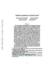
The non-cellular protists do not undertake self-reproduction; instead they direct their reproduction within another cell tenm the host. Cyan bacteria are classified another group of microorganisms, although they are often considered to be included with ether bacteria. Fungi are divided into lower fungi, slime moulds and higher fungi which comprise yeasts. Yeasts are free-living, single cells which they closely resemble fungi. Protozoa are living, organisms which although not generally engaged for biotechnology processes have been included for comprehensiveness. Viruses can be regarded as intracellular parasites. Growth of organisms involve multifaceted energy based processes. The rate of growth of micro-organisms is needy upon more than a few culture conditions, which should supply for the energy required for various chemical reactions. The speed of production of microorganisms and hence the fusion of a range of chemical compounds under artificial culture, requires organism specific chemical compound as the reproduction medium. The kinds and relative concentrations of ingredients of the medium, temperature. pH. dissolved oxygen, flow rate, volume etc pressure microbial growth. 12
2.2.2
Fermentation process phases After the inoculation of a nutrient solution with microorganisms and cultivation under physiological conditions, four phases of growth can be observed, •
Lag phase
Physiochemical equilibrium between microorganisms and the environment inoculation with very little growth, •
Log phase
At the end of the lag phase cells have modified to the new environment of growth, Growth of the cell mass is now described quantitatively as a repetition of cell number per unit time for bacteria and yeasts, Plotting the number of cells, biomass against time on a semi logarithmic graph, a straight line will results, Although the cells adjust the medium through uptake of substrate and emission of metabolic products, the growth of cells remain steady at this phase and is independent on substrate concentration as long as surplus substrate is there. •
Stationary phase
As soon poisonous substances have been created, growth slows down. The biomass increases steadily, although the composition of cells may alter. Various metabolite created in this phase are often of biological interests. •
Death phase
In this stage the energy reserves of the cells are worn out A straight line may be obtained when a semi logarithmic plot is made of survivors versus time, indicating that the cells are dying at an exponential rate. The length of time between the stationary phase and death phase depend on the microorganism and the process used. Fermentation is episodic at the end of the leg phase or before death phase begins All four growth phases are observed on Figure 2.2
13
:D
= =
~
~ = l'l ~
=
~
Jg
!"-
~
5:
~
8
=
= =
~
3':
=
::g
£;
=
Time
Figure 2.2: Growth curve of a bacterial culture
In industry fermentation is a process that takes place in tanks called bioreactors or fermentors. A typical industrial fermentation and typical process measurements that are available are shown on Figure 2.3.
Batch. continuous Process Inout
On-line measured
and fed-batch
Process Outputs
Fermentor
Uti-line measured Figure 2.3: Typical industrial fermentation
It is important to distinguish between those process variables measurements that can be made off-line and on-line. Process inputs are substrate flow-rate, Heat on or off, etc. Online environmental control are, temperature, pH, etc), and off-line environmental control are, biomass concentration, product concentration and substrate concentration. Off-line measurements are made by process operators taking a sample of broth and awaiting results from laboratory before making corrections to the process inputs. The fermentation process can be operated in either batch, fed-batch or continuous fermentors.
2.2.3
Comparison of fermentation processes Fed-batch bioreactors have a number of well known advantages over batch or continuous fermentors (Banga et al., 2002). For example, fed-batch can be the best (or even only) alternative due to its effectiveness in overcoming undesired effects like substrate inhibition and catabolite repression. Besides, it provides better control of deviations in the organism's growth pattern and production of high cell densities can be possible due to extension of process time, which is useful for the production of
14
substances associated with growth. An illustrative example of the importance of the fedbatch culture is the large' scale production of monoclonal antibodies, with product revenues in USA of several billions of USD (Bibila and Robison, 1994). 2.3
Modeling offermentation processes Fermentation processes are dynamic, non-linear and non stationary, in nature, thus leading to many difficulties in modeling. Modeling of biological processes has always been somewhat challenge. However, it is neither necessary nor desirable to construct comprehensive mechanistic process models that can describe the system in all possible situations with a high accuracy (Galvanauskas et al., 1998). In order to optimize a real biotechnical production process, the model must be regarded as a vehicle to reach more easily to the final aim. The model must describe those aspects of the process that significantly affect the process performance. Modeling must be leaning at the optimization task to be solved and must not uncritically sample all the information available about the microbial system used. From the theoretical point of view, the model describes the possible paths of the process through state-space representation. The system is non-linear and time varying, state equation are written as (2.1 )
xU) = a(x(t),u(t),t)
Where x(t) is the state vector andu(t) is the control vector. The easiest modeling concept presumes ideal mixing, which is rarely, if ever achieved. The asepticity necessity create measurements from the fermentor non-trivial. Cellular process, mass transfer and control aspects make the modeling appears more devastating, and thus it should cautiously be considered, what actually needs to be modeled given exact problem. Different techniques have been developed in recent years for different modeling needs. Some focus on the reactor, some on reaction kinetics (Eungdamrong and Iyengar, 2004). and some on system biology: metabolomics, proteomics (Goesman et al., 2003; Klein et al., 2002; Lemerle et al., 2005). Lack of specific sensors makes certain variables unreachable by on-line measurements. The difficulties experienced by control engineers when studying these types of processes, result from the fact that the process model is based on nonlinear algebraic relations and differential equations. These difficulties make the biotechnological process an excellent field for application of advanced control (Dahhou et al., 1991a).
15
2.4
Modeling Approaches To be able to control an industrial process it is required to know the relationship between the unprocessed material, process settings and end-product results (Jorgensen and Naes, 2004). Measured input parameters can be mathematically modeled to end product attributes, without any prior knowledge or hypothesis of their contribution to those endproduct attributes. The use of predictive modeling methodologies can be used to build predictive models for target responses (Estrada-Flores et al., 2006). There are three modeling approaches that were studied in the manufacturing of dairy products (Peter Roupas, 2008) namely • • •
2.4.1
White box models Black box models Grey box models
White box models White box modeling approaches are described as mechanistic, first principle, hypothetico-deductive, phenomenological, or state-space modeling. These approaches are based on the knowledge and fundamental theoretical principles of the process or factor being modeled and universal equations can be applied to build the model. Such models are applicable over any range of conditions or which model assumptions hold. Values of the input data are independent of measured and the accuracy of the model and the validity of its assumptions and underlying theory, are tested against the real-world measurements of the modeled process (Estrada-Flores et aI., 2006).
2.4.2
Black-box models Black box modeling approaches are empirical, inductive or input/output modeling and are useful when the mechanisms underlying a systems behavior are unknown or poorly understood, or where known mechanisms are too complex to be modeled efficiently from first principle. Examples of this approach include multiple regression models or Artificial Neural networks (ANN) models that require no theoretical basis. Black box models are developed from actual world information (Estrada-Flores et al., 2006) and have been proven to be particularly helpful where serious parameters are identified and measured on-line (O'Callaghan and Cunningham, 2005).
16
2.4.3
Grey-box model A grey box, or hybrid modeling approach combines the use of first principle based whitebox models and database black box models, and is particularly useful when there is a lack of fundamental theory to describe the system, or process being modeled, when there is a limited experimental data for validation, or when there is a need to decrease the complexity of the model. This model approach has been used to create mathematical models to predict the shelf life of chilled products or the thermal behavior of imperfectly mixed fluids or to create Artificial Neural Networks (ANNs) and dynamic differential equations for control-related applications (Estrada-Flores et al., 2006). It has an advantage over white box in that it provides a way around missing information in a complex system and performance from a control point of view (O'Callaqhan and Cunningham, 2005). It has been reported that such grey-box solution have not perform the separate white and black models in terms of predictive precision for explicit applications (Jones and Brown, 2007). The grey box modeling gives opportunities to illustrate in a better way the performance of the fermentation processes. The capability to predict the perfomrance of fermentation systems enhances the possibility of optimizing their performance. Mathematical expressions of model systems symbolize a tool for this and the most modern advances in computer hardware and software have made the approach more helpful than previous basic attempts. The current information of biochemical microbial pathways and the experience in optimization of chemical fermentors combined with very powerful and easily reached computers, loaded with easy to use software and mathematical routines, are changing the way processes are being developed and operated. This possibility is investigated in the thesis by development of mathematical models and decomposition methods for calculation of optimal control of all three types of the fermentation processes using parallel computation in a cluster of computers.
2.5
Kinetic models Kinetic modeling expresses the verbally or mathematically expressed correlation between rates and reactanUproduct concentrations, that when inserted into the mass balances, permits a prediction of the degree of conversion of substrates and the yield of individual product at other operating conditions( Nielsen and Villadsen, 1992). Kinetic model is nomrally a black box model and can be shown diagrammatically by the structure on Figure 2.4.
17
s (t) Kinetic x(t) p(t)
model
JI(t)
~
Figure 2A: Kinetic mode! structure
Where set) is substrate concentration, pet) is a product concentration, x(t) is a biomass concentration and !J(t) is the growth rate of microorganisms. If the rate expressions are correctly set up, it may be possible to express the course of an entire fermentation experiment based on the initial values for the components of state vector, e.g., concentration of substrate. The basis of modeling is to express functional relationship between the forward reaction rates of the reactions considered in the model and the concentration of the substrates, metabolic products and biomass: f.li
= fi(s,p,x)
(2.2)
Where Jh is the forward reaction rate. A good understanding of the kinetics in terms of mathematical modeling is an important step in developing a successful control strategy. It is often possible to accurately represent the growth of microorganism, which is an unusually complex phenomenon by relatively simple empirical models. One of the most important factors influencing the growth of Sachoromyces cerevisiae is the effect of specific inhibitors. During ethanol fermentation, in general both product and substrate inhibitions can be considered as significant. An extensive literature review on alcohol tolerance of the microorganisms has been presented by (Casey and Ingledew, 1986). (D'Amore and Stewart, 1987), (Jones, 1989), (Pamment, 1989) and (Warren et ai, 1992) have also presented a review of literature on ethanol inhibition. Ethanol inhibition has been modeled in general by its effect on two parameters: • •
The specific growth rate of the microorganisms The specific product formation rate
Both models can be well thought-out as important in the case of batch fermentations since these models can predict ethanol production in the lack of growth of the microorganism Kinetic models are investigationally derived mathematical formulas that fit the measured data reasonably well. The easiest kinetic modeling practice is the application of an unstructured kinetic model. The kinetics can be linear or nonlinear, single-phase or 18
multiple phase (Eungdamrong and Iyengar, 2004), (Mitchel et aI., 2004). Linear kinetic models take account of constant rate and first order kinetics. Nonlinear kinetic models comprise exponential, logistics, second order other defined functions (Eungdamrong and Iyengar, 2004), (Maurer and Rittmann, 2004) and (Mitchel et al., 2004). The mainly accepted defined kinetic model function has certainly been the Monod model, which contains two parameters that define the relation of growth and substrate utilization. The Monod model was the foremost unstructured mechanistic model. It can be considered as the mainly basic model to describe the growth of a given microorganism in the absence of any specific inhibition effects. This model is based on the hypothesis that the growth is restricted by a single substrate concentration and is given by:
f1=
J.1 max K, +
S
(2.3)
S
Where JG is the Monod constant, substrate concentration
[g/~.
j-lmex
is the maximum specific growth rate and s is the
The importance of JG is that when substrate concentration
is numerically equal to JG growth rate is exactly half of the maximum growth rate. In many systems the product inhibits the rate of growth. The equation that is used to represent the
product inhibition on the growth rate is {Dochan et aI., 1990
rg = (l_~)n(f1maxxs) p
Where
rg
(2.4)
K,+s
is the cell qrowth rate,
x is
the cell concentration,
p' is the product
concentration at which all metabolism cease and n is the empirical constant for Saccharomyces cerevicerae. The investigations on the thesis are based on the kinetic model (2.4). Maximum specific grovvth rate is expressed as function of ethanol concentration. In other words the overall effect of ethanol inhibition on growth rate can be accounted by adjusting growth rate in above. Contois and Moser (Kiviharju et al., 2007) presented modifications to the Monod model. Contois theory was base on increase inhibition by biomass itself, which has later been doubted (Nielsen and Villadsen, 1994). Other different formulas were presented by Teisser and Blackman (Kiviharju et al.. 2007). The logistics expression has also been successfully used in the gro'A'lh estimations. The Monod model has also been extended to substrate and product inhibition (Nielsen and Viliadsen, 1994). These, however have more parameters and require more computing 19
power to fit appropriately. Kinetic models have been applied to the lag and death phases and in particle interactions (Mitchel et al., 2004). Temperature and PH can change the activities of many enzymes and influence the growth kinetics (Maurer and Rittmann, 2004), (Mitchel et al.. 2004) and (Nielsen and Villadsen, 1994). The above mentioned models are all empirical expressions, it is futile to debate which one is the best, simply choose the one that best fits the system. Some of the kinetic models are given below: Tessier model
J1=J1max (1 - ( e ) - ' IK' )
(2.5)
Where s is the concentration of substrate Moser model
(2.6)
Where n is the empirical constant for Saccharomyces cerevicerae Contois model
J1=
JL rna\": S K,x + S
(2.7)
Blackman model
{.u
J1 =
max
2~;s ,,; 2K,
).t max
2.6
S ~
(2.8)
ZIG
Mass balance principle of fermentation processes In modern approaches to fermentation control, a reasonably accurate mathematical model of the reaction and reactor environment is required. Using process models, progress beyond environmental control of bioreactors into the realm of direct biological control can be achieved. Development of fermentation models is aided by information from measurements taken during the process operation. Models are mathematical relationship between variables. For biological processes, specifying the model structure can be very difficult because of the complexity of cellular processes and the large number of environmental factors which affect the cell culture. 20
Process models vary in form but have the unifying feature, that they predict outputs from set of inputs. Another important factor affecting reactor performance is the mode of operation such as batch, fed-batch and continuous. Choice of operating strategy has an effect on substrate conversion, product concentration, susceptibility for contamination and process reliability. The dynamic behavior of the growth of one population of microorganisms on a single limiting substrate in a stirred tank reactor is most often expressed by equations (Dochan and Bastin, 1990) which are obtained from straight forward mass balances: ~._._._._._._._.~
r'-'-'-'-'-'-'-'~
, The rate of mass in through
,
I
The rate of
, mass out ;+! ,.. ,,. , through !
system
system
boundaries.
boundaries
~._._._._.-._._
..
'-'---'---'---''''j
' , ,H-i,
,._. _. _._. _. _. _. _.1
~ . _ . _ . _ . _ . _ . _ . _ . ,
Mass generated
'-'---'-'-'---'-'1
The rate of
The rate of
J
,
-
mass
'_, Mass
consumed
!-; accumulate , d
within
within
system.
system.
,;._._._-_._._._)'
The rate of
within
,
~'-'-'-'-'-'-'-'-'
system. 1._.
._. _,_, _._.1
Mathematically (2.9) can be written by the following equation
dM(t) dt
AIt(t)-Mo(t)+RG(t)-Rc(t),lvf(O) = Af¢where t is the time
(2.10)
M = mass of component in the vessel
M. = mass flow rate of component entering the vessel M,
=mass flow rate of component leaving the vessel
RG = mass rate of generation of component by reaction Rc = mass rate of consumption by reaction
M, = Initial mass of the component in the vessel The mass balance equation can be written for a separate component, or for the whole process. This equation is used to develop the unstructured models of the different types of fermentation processes. Three equations form the corresponding model of the fermentation processes. They describe the mass balances for the biomass. substrate and the product. Equations are derived under the following assumptions • •
Stirred tank reactor The process is assumed to be in complete mixed conditions: this implies that the composition of the medium is homogeneous in the reactor. 21
•
2.6.1
The biomass growth and the substrate consumption are propositional to the biomass concentration and are described below for every type of fermentation process.
Models for Batch fennentation process Batch processes operate in a closed system; substrate is added at the beginning of the process and product is removed only at the end of the process. It is assumed that the reactor has no leaks and evaporation meaning the volume of the vessel V is constant. •
Derivation of the biomass equation
Assuming well mixed batch fermenter for cell culture or biomass concentration x and applying mass balance equation (2.10), it can be written The reactor has no input and output which means that
At = M: = 0
(2.11)
Mass of ce!Js in the reactor is equal to the product of the concentration of the biomass and volume.
M=xV
(2.12)
Mass rate of cell growth RG is equal to r,V (2.13) Where r, is equal to f1X, r» is the volumetric rate of growth, fl is the specific grolA'!h rate of the microorganisms, which can be expressed by Monod kinetic law in (2.3). If cell death takes place in the reactor, the mass rate of consumption of biomass is given by
Rc=rdV
(2.14)
Where ra = ksx is the death of microorganisms and ks is the death constant. Then following equation (2.10) where
M=xV d(xV) =o In-V -kdxV.. ,ro
(2.15)
x(O) = x» (2.16)
at
22
Taking derivatives of equation (2.16)
xd(V) Vd(x) -'----'-+--
dt
dt
= xV(j1-lCd),x(O)=x.
(2.17)
Since the volume of the reactor is constant, dV
dt
=0
and the mass balance equation for
the biomass is
d~? = x(j1-lCd), •
x(O) = x» (2.18)
Derivation of the mass balance equation for the limiting substrate
The reactor has no input and output which means that mass flow rate entering the reactor is equal to the mass flow rate leaving the reactor and equal to zero, which is given by equation (2.11). The mass of substrate in the reactor is
M=sV Where
(219)
s is the substrate concentration and V the volume of the Reactor
No substrate generation in the reactor RG = O. The substrate is consumed by the microorganisms in the reactor
Rc = r.V
(2.20)
Where r, is the rate of consumption, which depends on the specific growth rate, the yield coefficient E" and the coefficient of maintenance of microorganisms m. and biomass concentration x
(2.21) Then
Rc =
_(
~ +m,)xv
1.1"
(2.22)
Applying equation (2.10) the substrate mass balance equation describes only substrate consumption
23
d(sV) dt
= _(L+m,)xV YlS
(2.23)
Taking derivatives of equation (2.23) d(s) (f.lm"S ) ---:it = - E,,(K. + s) + m, x,
•
s(O)=s" (2.24)
Derivation of mass balance equation for the product concentration
The reactor has no input and output which means that mass flow rate entering the reactor is equal to the mass flow rate leaving the reactor and equal to zero, which is given by equation (2.11). The mass of product in the reactor is
M=pV
(2.25)
No product consumption in the reactor
R c = 0 Generation of the product in the reactor is (2.26) Where rp is equal to qp> Vmax
wherev
s-
x.scp, k=O,K, v=T, k=O,K-l 60
The obtained values of the trajectories of the state and control variables are function of the coordinating variables. They are optimal for the given values of the ooordinating variables. If the coordinating trajectories are optimal ones, then the obtained state and control variables also will be the optimal according to the theory of the duality in optimal control and Lagrange methods. 4.3.4
The coordinating sub-problem for batch fermentation process The coordinating variables are obtained from the necessary conditions for optimality of the augmented Lagrange functional according to them. For the conjugate variables these are equations (4.9)-(4.11). The necessary conditions for optimality according to the new introduced interconnections in time domain are:
oL
(4.35)
oO,(k)
oL
-A,(k) -,u, [- 5, (k) + !,(k)] = -A, (k) - ,u,e} .s (k)
00, (k)
=
eo, (k)
=
0,
(4.36)
(4.37)
where
-5
V(k)+
f(k)=e1v(k),v=x,s,P.
according to equations (4.9)-(4.11). The necessary conditions for optimality (4.9)-(4.11) and (4.35)-(4.37) can be combined in a gradient procedure. Equations (4.35)-(4.37) give the values of the gradients for the conjugate variables multiplied by the penalty coefficient.
u.: v = x, s, p
It appears that:
oL
oov(k)
=-A k _ oL k=O.K-I v(),uv 0 Av(k)' .
(438)
Gradient procedure can be built for both type of coordinating variables, as follows: For conjugate variables: (4.39) 61
where
e J ).v(k) = -0/ (k)+ F v(k),v = x,s,p, k = O,K -1,
(440) (441)
where
Cl"J.,.
and a"-vare the steps of the procedures for calculation of the conjugate
variables and the interconnection in time, respectively. As the calculations are based on gradient iterative procedure, they will stop when the gradient is going to zero, or practically achieving some conditions for optimality, given by
k=OK , (4.42) where E1jv,
I: J.v
are a very small positive numbers. For every step of the gradient
procedure for the coordinating process the full iteration cycle of the sub problems of the first level is done. The calculations of the coordinating variables are done with the values of state and control variables of the first level sub problems and the calculations of the first level sub problems are done with the values of the calculated on the previous iteration coordinating variables. The iterative process of coordination and the optimal solution of the whole problem for optimal control is obtained when the optimal solution of the coordinating sub problem is reached, this means conditions (442) are fulfilled and if these conditions are not reached the error is computed. (4.43)
The new penalty coefficient is calculated from the conditions.
if j
= lOT e j +1 < e j , then /-lj+1 = /-lj
(4.44) (4.45)
4.4
Algorithm of the Augmented Lagrange for batch fermentation process The calculations in the two-level structure can be grouped and represented in the following algorithm:
62
1. On the coordinating level the initial values of the coordinating and gradient procedures, variables and parameters, initial trajectories of the state, control and coordinating variables are set as follows: • • •
Maximal number of step of the coordinating process - M2. Maximal number of steps for state and control variables gradient procedure- Mi. Steps ofthe gradient procedures For coordinating conjugate variables -a A,.' v = x,s, p . For coordinating interconnection in time aJ,.,v = x,s,p
•
For state variables and control variable a,., v = x, s, p, T Values for error and termination of the calculations for coordinating procedures. £;.,.,£",., v = x.si p and for gradient procedures on first level.
£,.,v • • • • •
•
=
x,s,p,T
Initial trajectories of the conjugate variables . .,1\ (k), v = x.s, p.k = O,K -1 Initial values of the state variables, x(O), s(O), p(O). Number of steps in the optimization horizon - K and value of the sampling period M. Initial trajectories of the control variables TUCk), k = 0, K - 1 The initial trajectories of the control variables are substituted in the model equations (2.81)-(2.83) and (2.72)-(2.75) and the state trajectories are calculated. The initial trajectories of the interconnections in time domain are calculated from o,.(k) = v(k+ l),k = 0,K-1
• •
Initial trajectories of the coordinating variables and initial state and control trajectories are sent to the first level. Coefficients of the model a, --+a3, b ,--+b3 , c- --+ C3, and d, --+ d 3 , ! 0, v = x,s, p,V,F,T,k = O,K -1
(5.37)
The values of the state variables, the final point are calculated from the optimal values at the previous point according to equation (5.18). The new calculated values have to be checked for belonging to the area of constraints.
88
(5.38) (5.39)
(5.40)
V min ~ V(k) F min
~
F(k)
~ ~
V min, k = O,K
(5.41)
F max, k = O,K - I
(5.42) (5.43)
Simple way to do and correct the obtained new values is to project them over the constraints domain according to the relation:
if yJ.i (k) < y min yi.' (k), if y min ~ yi., (k) ~ y max'
y min' yi., (k) =
(5.44)
yiJ(k) > y max
k=O,K forv=x,s,p,V andk=O,K-l for v=T,F The obtained values of the trajectories of the state and control variables are function of the coordinating variables. They are optimal for the given values of the coordinating variables. If the coordinating trajectories are optimal ones, then the obtained state and control variables also will be the optimal according to the theory of the duality in optimal control and Lagrange methods. The optimal values of the coordinating variables are obtained by the solution of the coordinating problem. 5.3.4
The coordinating sub-problem for fed-batch fermentation process The coordinating variables are obtained from the necessary conditions for optimality of the augmented Lagrange functional according to them. For the conjugate variables these are equations (5.11)-(5.14). The necessary conditions for optimality according to the new introduced interconnections in time domain are:
oL
(5.45)
oJ,(k)
89
oL
-2,(k) - ,u,[o, (k) - I, (k)] = -2,(k) - ,u,e2 , (k)
oO,(k)
= e 5 , (k) =
°
(5.46)
(5.47)
oL
-2, (k) -,u, [0, (k) - !,(k)] = -2, (k) - ,u,e;., (k)
oov(k)
= eo,'(k) =
°
(5.48)
where 0v(k) - fr,(k) = eAv(k), v = x, s.p, Vaccording to equations (5.11)-(5.14). The necessary conditions for optimality (5.11)-(5.14) and (5.44)-(5.47) can be combined in a gradient procedure. Equations (5.44)-(5.47) give the values of the gradients for the conjugate variables multiplied by the penalty co-efficient. ,uv' v = x,s,p,V It appears that
oL
(5.49)
oov(k) Gradient procedure can be built for both type of coordinating variables. For conjugate variables:
• i+1(k) -
A]!
-
1 /,,,,~,
i(k) -a.l~,e 1.. . I! (k) ,
(5.50)
where
e' J.,.(k) = -5/ (k) + F v (k), v
= x,s,p,v,k = O,K -1,
(551) (5.52)
where a 2v and aJvare the steps of the procedures for calculation of the conjugate variables and the interconnection in time, respectively. As the calculations are based on gradient iterative procedure, they will stop when the gradient is going to zero, or practically achieving some conditions for optimality, given by
lIej+1Av(k) - ejAv(k)
II : : ; EAV,EAV > O,k = O,K
Ile j+1 ov (k ) -
II s
e j ov(k)
Eov' Eov
> 0, k =
0, K -1
90
(5.53)
where Eav' &1" are a very small positive numbers. For every step of the gradient procedure for the coordinating process the full iteration cycle of the sub problems of the first level is done. The calculations of the coordinating variables are done with the values of state and control variables of the first level sub problems and the calculations of the first level sub problems are done with the values of the calculated on the previous iteration coordinating variables. The iterative process of coordination and the optimal solution of the whole problem for optimal control is obtained when the optimal solution of the coordinating sub problem is reached, this means conditions (5.52) are fulfilled and if this condition is not reached the error is computed. (5.54) The new penalty coefficient is calculated from the conditions.
5.4
if j
= lor ei +1 < ei .theti Jli+1 = Jli
if j
> land ei +1
;:::
(5.55)
ei then Jli+ 1 = a/l i , a = [0.1 10.0]
(5.56)
Algorithm of the method for fed-batch fermentation process The calculations in the two-level structure can be grouped and represented In the following algorithm: On the coordinating level the initial values of the coordinating and gradient procedures, initial trajectories of the state, control and coordinating variables are set as follows: • • •
Maximal number of step of the coordinating process - M2. Maximal number of steps for state and control variables gradient procedure- M1. Steps of the gradient procedures For coordinating conjugate variables -a1,.,v = x,s,p,V. For coordinating interconnection in time -a"",v =x,s,p,V . . For state variables and control variablea",v =x,s,p,T,F
•
•
Values for error and termination of the calculations for coordinating procedures. &"",sov'v = x.scp, V and for gradient procedures on first level. e., v = x,s, p, V Initial values trajectories of the conjugate variables.
2'v(k), v
= x,s,p, V,k = 0, K -1
• •
Initial values of the state variables, x(O), s(O), p(O) and V(O). Number of steps in the optimization horizon - K.
•
Initial trajectories of the control variables T
91
11 •
(k), F
1,1(k),k
= O,K -1
•
• •
The initial trajectories of the control variables are substituted in the model equations (2.88)-(2.91) and (2.72)-(2.75) and the state trajectories are calculated. The initial trajectories of the interconnections in time domain are calculated from o,,(k) = v(k+ 1),k = O,K -1, v = X,S,p, V Initial trajectories of the coordinating variables and initial state and control trajectories are sent to the first level.
2. On the first level the following calculations are done: • •
Derivatives of equations (4.8) are calculated. The kinetic coefficients,umax,K"Y""Ypxfrom equations (2.72)-(2.75) are calculated.
•
The
expressions
rpx(k),rp,(k),rpp(k),rjJv,rp, (k),rp2(k),k = O,K -1
are
calculated from equations (5.25)-(5.30). • •
• •
The gradientse/' (k),k = O,K ~ 1, v = x,s,p,V,F,T are calculated from equations (5.31)-(5.36). The errors for the end of the gradient procedures are calculated according to equation (5.37). If the error is less than G v ' the calculations of the first level stop and the current values of the state and control variables are the optimal ones. If the error conditions are not satisfied the new values of the state and control values are calculated. The new values of state and control variables are calculated from equation (5.18). The obtained state and control variables are projected over the constraint domain according to equation (5.44). The obtained trajectories are sent to the second level.
3. On the second level the following calculations are done: •
The final value of state trajectories v(k) are calculated
•
The
•
• •
gradients
e;.v(k),k=O,K-1,v=x,s,p,Vare
calculated
from
equations (5.11 )-(5.14). The conditions for the end of the calculations are checked according to Equation (5.53). If the conditions are fulfilled the optimal solution of the coordinating and of the whole problem are obtained. If the conditions are not satisfied the new values of the coordinating variables are calculated. New values of the conjugate variables are calculated according to equation (5.50)-(5.51). The new values of the interconnections are calculated from equation (5.52). These trajectories are sent to the first level sub problems where the calculations from p.2a till 3b are repeated and so on. The schematic diagram of the algorithm is given on Fig 5.1
92
Set initial values
°
}c,. (k),
u., x(O),s(O),p(O),v(O) Setup
FO (k),To (k), k=O,K-1 Calculation of initial state trajectories V
O
(k + l),k = O,K
... = }.O (k), Sf (k) = SI(k) Vf,i (k) = VO (k), v = X,S, p, V,F,T )/ (k)
I
$ T
Calculation of state and control derivatives, Equations (54)-(510)
~ Calculation of kinetic coefficients. Equations (2.72)-(2.75)
Calculation of expressions:
q;/.i '¢1'¢"
k
= O,K-1
~ Calculation eJ·".(k) from equations (5.31)-(5.35)
~ 1
Calculation lief.' v
(k)11 from equations (5.36)
I 93
1
Yes
v = x,s,p, V,F,T
No
Vi,! (k) = V =
vi,' (k) + a i ,! v (k)
x,s,p,V,F,T
Projection on constraint domain Equation (5,43)
Calculation of Equations (5,11)-(5.14)
e' Av(k),},v = Ax,A"}"D,A, Calculation of llei,!
",,(k)11 equation (5.52) N
l
Calculation Ai + v(k),
sr', (k)
Equation (5,49)-(550)
No v(k) = vi'! (k) V
=
x,s,p,V,F,T STOP
Yes
Figure 5.1: Flow chart of the algorithm for calculation of optimal trajectories of fed-batch
fermentation process
94
5.5
Description and calculation results from the sequential program of the algorithm of the method in Matlab for fed-batch fermentation process The algorithm presented in section 5.4 is implemented in Matlab in a sequential way(Appendix 8). The table below represents the relationship between mathematical notation and program notation of the Matlab program. Table 5.1: Correspondence between mathematical and programs notations for ~,~;~atch fermentation "", State variable Biomass
x
x
Substrate
s
s
Product
p
p
volume
v
v
Control variable Temperature
T
T
F
IF
Flow rate Steps of the gradient procedures For state variables
ax
ax
as
as
"p
ap
",
av alx
",Ix
,
Conjugate variable
".Is
als
".!p
alp
".Iv
alv
alix
adx
"lis
ads
aliv
adv Ix
Ax As Ap
,
Is
liP !v
)",
95
I
Interconnections in timedomain
Coefficients
J,
dx
J,
ds
Jp
dp
J,
dv
az. 83
a1, a2, a3
b" bz, b,
b1, b2, b3
C1, Cz, C3
c1,o2,c3
d" da, d,
d1, d2,d3
K"
Kd
al,
,
Ks
K,
m
.
m
n
n
v;
Yxs
Yp,
Ypx
s,
51
P
pi
M
dt mmax
flrn:.Lx Initial values of statevariables
Penalty coefficients
x(O)
xO
s(O)
sO
p(O)
pO
v(O)
vO mx
fl."
ms
fl.,
mp
fl. p
mv
fl.,
xmax
Min and max of Xm", state variables Xmin
xmin
Sm",
smax
Smin
smin
pm",
pmax
96
Min and max of control variables
Derivaives of the model parameters
pmin
pmin
Vm~
vmax
Vmjn
vmin
Tm~
Tmax
Tmin
Tmin
Fm~
Fmax
Fmin
Fmin a2+2*a3*T(k);
ap ar"' =a1 +2a,T(k)
dmmaxdT(k)
aK a; =b1 +2b3T(k)
dKsdT(k)-b2+2*b3*T(k);
a}~s
dYxsdT(k)-c2+2*c3'T(k);
.
aT
ay a;'
,
= C2 + 2c,T(k) dYpxdT(k)-d2+2*d3*T(k);
= d 2 + 2d,T(k) I
Error
e;s(k)
ax(k)-x(k+1)
elx(k) - dx(k)-x(k+1)
e;s(k)
8s(k)
s(k + 1)
els(k) - ds(k)-s(k+1)
e;p(k)
ap(k)
p(k+1)
elp(k) - dp(k)-p(k+1)
e,(v(k) - 8v(k) - v(k + 1)
elv(k) = dv(k)-v(k+1) edx(k)=-Ix-mx*elx(k)
e",(k) --}'x - px(k)e;./ (k)
eds(k) -Ix-ms*els(k)
e"" (k) - -Ax - p, (k)e;./ (k)
edp(k)-Ix-mp'elp(k)
e,,,,(k) - -Ax - pp(k)e;./ (k)
edv(k)--Ix-mv*elv(k)
e",(k) - -Ax - f-l,(k)e;./ (k)
.
Formulas
ff(k)=dt*mmax(k)*( (1pklpl)'O.52)
[7 J
MPmax 1-
p(k)
MPmax [1- p(k) p*
Mf-lm" [1- p(k) p*
= ((Jf(k)
r
fx(k)-ff(k)'s(k)/(Ks(k) + s(k))
s(k) K, +s(k)
((Jx(k)
x(k)s(k) [K, + S(k)]"
=
J
97
(k) ({J,
fs(k)-ff(k)'Ks(k)' x(k)/((Ks(k) + S(k))A2)
I
/';/ [1-
p(k)
P*
fima,
/';/[1- p(k) fi
5.6
m"
rpp (k)
fp(k)-dt*mmax(k) *((1p(k)!pl)'(n1)tx(k)*s(k)!(pl*(Ks(k)+ s(k)))
rpv(k)
V'(k)
/';/ [1-
n -1 x(k)s(k) P. K s +s (k)
fv(k)=dt*F(k)!(v(k)'2)
Sr F(k)
p*
r'
J
x(k)s(k) K, +s(k)
p(k) p*
9, (k)
J
x(k)s(k) = (k) [Ks+s(k)f rpz
f1(k);ff(k)*x(k)*s(k)!(Ks(k) .;s(k))
f2(k)=f1 (k)!«Ks(k).;- s(k»))"2
Description of the Matlab sequential program for optimal control of fed-batch fermentation process The complex relationship between physiochemical and biological variables and sudden unexplained changes in the process are reflected in the values of the equation kinetic parameters equations (2.72)-(2.75) which are the same as from section 4.6. Table 5.2 defines process kinetic values that are calculated from Matlab by using polyfit function from a certain given values of the equation kinetic parameters. Program fedbatch_seque.m is developed to implement the decomposition method in a sequential way. The program calculates the optimal values of the state and control variables according to the algorithm 5.4. The whole program is in appendix B. The function modelfedbatch_func2 is used to calculate the trajectories of the derivatives of the state space vector, according to the Equations (2.84 - 2.86). Then the program is called by the solver ode15s for integration of the model equations. The input variables are t the time at moment t from the considered time interval, y initial. or value of the state vector in the moment t The output variables are the values of the state space vector derivatives ydot. The program is given in appendix B.
98
..
Table 5 2' Model parameter values for fed-batch process Symbol Name Value I a1 Model co-efficient 0.0004 a2 Model co-efficient 00001 a3 Model co-efficient 0.0002 Model co-efficient b1 0.2 Model co-efficient b2 0.03 b3 Model co-efficient 0.01 Model co-efficient c1 2 c2 Model co-efficient 0.3 Model co-efficient c3 0.021 d1 Model co-efficient 00360 Model co-efficient d2 0008 Model co-efficient d3 0.003 Death constant Kd 000008 Inhibition factor p". pi 50 n Powerc-oefficient 052 Maintenance-coefficient m 0.0011 Biomass concentration x Substrate concentration s Product concentration p Sampling period dt 0.25 . Maximum grmvth rate Umax Monod's constant K, Stochiometry coefficient fer biomass growth
Unit
gil
gil all
v;
5.6.1
Results from sequential calculation offed-batch fermentation process The program for sequential calculation is used to calculate the optimal trajectories of the control and state variables ofthe fed-batch fermentation process. The optimal trajectories are presented in figure 5.2 -5.9
99
Initial tlajedorie; ctstate>alables
160
14J",,, 120 ~ \, ,, , 100~
'" CfI
EOl 6"3 40' 201-
25,
--biomass - - - - - -sutGtrate - - - prooucl - volu!Til
O/iimis a:t Results fer the bioma;s state , " , I-biomass
20
f
,,
,, , ,, ,
15
,, ,,
'ii
,, ,, ,
10
,, :,
OL-A ----- -
~=~=~~-;:-;-;;-- ~ -- ~ ~~- ~ ..
-20'
a
, 5;0
, , 100 150 ZJO time insamples I
0 0
!
250
50
100 1m 200 lime insamplE!S
250
300
Figure 5.3: Optimal trajectory of biomass for fed-batch fermentation process
Figure 5.2: Initial trajectories of state variables for fed-batch fermentation process
100
I
Qiimised R€Sulis 1\I tre D"o:Iuctstate 6.
f
o plimised Resuns lorthe substrate
I----- D"o:Iuct I
,
5
160
1~~
I-substrate
120
.. -
4
~.
-- -
~ ~ ~~
-- - -- -- - - - - - --- _.
,,•
100
.,
a, 80
. ,,
~J
,,
60 Z
4IJ
, ,,, , ,,
20
50
1W 150 200 tin"e in sampl",
2'".:0
Figure 5.4: Optimal trajectory of product for fed-batch fermentation process
D D
Ell
100 15D 200 time rnsarnpes
Z5D
3DO
Figure 5.5: Optimal trajectory of substrate for fed-batch fermentation process
101
I
Optimised R15 ulls ftl the v:JIume stale
2.13,
I
2.12,·
~
R_~
R
Optim~oo
1- --v:JIume I
16,001,
\
i
ResulLs 1:1 the Temperallf€ T
1-- Ten1(Hallfe TI
i i i
16.0008
212 2.115~
160036
I
,
I
211
16.0804
r;
~
~
16.0002
2.185
1£
2.1
159:)98
z.u . ;'f,. 2 r9·") II
::::r\v, , ' , ,
2,0910 2UlU:!"
. u;./o
I
I
58
2!'iJ
o
338
ffi
loa
1!:(J
zoo
2!'iJ
j 3.10
time insamples
Figure 5.7: Optimal trajectory of temperature for fed-batch fermentation process
102
Optimised Resuns for the input flow rate F
31 25
i
i
i
r
1-
-Input flow rate F
15 f
••
'O.1~:~~1"
,
,
,
0
,
I
--lambiilX
- -- --
~
-
~
-
~
-
-- - --!.aroMa s
- - -!.ambia p - -lamJ:d'a \'
~I
,, ,,
\
.Qlf l, ,, ,, ""
I
""
JJJ~
\
0.5 f \ O~
0
ob-------.
\
"m
Opfuniooj ReS'flts br the cc~jugate \llriablffi lamJ:da
1\- [
11
2 f\ \
\
J).4
---------
.l15
-0.5 -1
1
0.1,
I
,
o
50
,
!
!
!
I
.4~.61
e
:YOO
Figure 5.8: Optimal trajectory of input-flow rate
~,
,, ,, ,, ,,, , ,,, ,, ,o •
· I
!
w
' -------------------~ r , !
1
l(}J 150 loo tim; mSImi'"'
2£0
!
31))
Figure 5.9: Optimal trajectory of conjugate variables
for fed-batch fermentation process
for fed-batch fermentation process
103
5.7
Discussion of the results for fed-batch fermentation process The biomass concentration generally continued to rise after feed was started, as at that stage growth rate exceeded dilution rate, but within few hours after increases in the feed rate. it invariably began to fall. Substarte levels generally rose slowly throughout the feed period as desired although it is fairly sensitive to feed rate, Product concentration on the other hand rises sharply for several hours after the feed was switched on and then reached a plateau, rising slowly after the feed was exhausted,
5.8
Conclusion This chapter describes the formulation of the problem for optimal control of a fedbatch fermentation process, An augmented Lagrange functional is used and a decomposition method for solving discrete time formulation of the problem is developed based on varational calculus and decomposition in time domain, The sequential algorithm of the decomposition method is describes and implemented in Matlab.The results are shown and discussed, The parallel implementation of the
decomposition method is described in chapter eight. The problem for optimal control of continuous fermentation process is considerd in chapter six,
104
CHAPTER SIX DEVELOPMENT OF A DECOMPOSITION METHOD FOR OPTIMAL CONTROL PROBLEM CALCULATION FOR CONTINOUS FERMENTATION PROCESS 6.1
Introduction The continuous process has some advantages when compared to the fed-batch and batch mode. If steady state is attained, quality of the final product is constant, as the operational conditions are invariable. Besides, the volume of the fermentor can typically be smaller, as shut-downs for harvesting and sterilization are less frequent. However, due to the high probability of contamination and culture degeneration caused by a long operational time, continuous processes are used only in few cases in the fermentation industry, such as cell mass and ethanol production. Before a continuous fermentor reaches stable state operation, there is a transient period in which it is filled up to the working volume. This is called the start-up of the fermentor and refers to the progression of operations that leads it from an original state to the final state of continuous operation. It is important to determine the efficient start-up strategy of the femnentor as it saves time. Bio-chemical reactions are typically slower than chemical reactions and an inappropriate start-up may cause the fermentor to spend time to reach the steady state conditions. The problem for minimum time control of continuous fermentation process is formulated in section 6.2 on the basis of a decomposition method. This method uses an augmented Lagrange functional in order to overcome the difficulties with the singular type of control and no quadratic criterion is developed in section 6.3. A coordination vector, constructed to achieve separability of the dual problem is developed. The problem for minimum time can be decomposed in time domain and be solved in a two level computing structure. A computer algorithm is developed to solve this problem in section 6.4.
6.2
Formulation of the problem for optimal control of continuous fermentation process The problem for minimizing start-up time of continuous fermentation process is considered (Tzoneva and Patarinska, 1995). The problem for minimum time is a dynamic one and the used model is dynamic (Tsoneva and Popchev, 1995). The aim is to minimize the time necessary for the process to reach steady state values of concentration of biomass, substrate and product. Mathematically, discrete minimum time
105
control problem for the continuous fermentation process is to find a control trajectory D(k).k = O.K -1 which in minimum time J=Kllt
(6.1)
leads the system presented by equations (2.96)- (2.98) and (2.72)-(2.75) from initial state x(O) =xo.s(O) =so,p(O) =Po to the optimal steady state x(K) =x, s(K) =s.p(K)
=p
while satisfying constraints for state and control variables xmin(k):S; x(k):S; xmax(k).k = O.K smin(k)
(6.2)
s s(k) s smax(k), k = O. K
(6.3)
Pmin(k):S; p(k) :s; Pmax(k). k = O,K Dmin(k):S; D(k)
(64)
s Dmax(k),k ~ O,K-1
(6.5)
and constraints for the sampling interval (6.6) Where Atmax is determined on the basis of stability requirements for the fermentation process
6.3
Decomposition method for optimal control problem solution for continuos fermentation process The considered problem for optimal control has the following characteristics • • • •
The objective is to minimize a function of the final time with a free final time starting from known initial conditions. For different initial conditions, different optimum for the minimum time values will be obtained. In the start-up of a continuous fermentation process the known conditions for the state equations are the final conditions. The stated problem is characterized by nonquadratic criterion and bilinear model with the control entering linearly the model equations
These characteristics determine which methodology to be selected for solution of the optimal control problem. The minimum time problem is transformed into a problem for minimizing the value of the sampling interval in the limits of (6.6). As the sampling period is easier to be included in the model equations and to be minimized, the number of sampling steps will then be fixed. The sampling period also enters linearly into the model equations. This means that the solution of the optimal control problem can be singular because the first derivative of the functional of Lagrange towards the control variable and 106
the sampling period will not include these variables. To overcome these difficulties an augmented functional of Lagrange proposed in (Tzoneva and Patarinska, 1995) is used to solve the problem.
La = Kilt + Lv:x,s,p 1)
ill
+ ~J.lv[V(K) - ilj2} + If;;;J Lv:x,s,p {l,,(k) [-v(k +
+ +ivCk)] + ~J.lv[-v(k + 1) + ivCk)j2}
where il =
6.3.1
{l" (K) [v(K) -
(67)
x,s,p
Necessary conditions for optimality for continuous fermentation process Solution of the problem for optimal control is based on the necessary conditions for optimality of the functional of Lagrange (6.7). The equations of these conditions are used to build the algorithm for calculation of the optimal state, control variables and sampling period. This algorithm is used for parallel calculation in a cluster of computers. •
Necessary conditions for optimality according to biomass
p(k)]n[ 8L =A. (k)[l+MJI [l_ s(k) ]-Mk -MD(k)]&(k) .r z-mex p* K, + s(k) d
-p,(k)[x(k+1)- Ix(k)][l+MPma,[l-
+}'s(kl Mpma, [l_
L Y",
p(k)]n[ p*
,s(k) K,+s(k)
p(k)]n[ s(k) ]-Mkd -MD(k)] + p* K, +s(k)
]-Mm]-
_ P, (k)[s(k + 1) _ f, (k)][MPmax [1- P(k)]" [
I:",
p(k) p*
p
*
s(k) K, +s(k)
+ ..... (k) M}pxJ.lmax [1 - - -]n[ ,
T
p
[
- P p (k)[p(k + 1)-
8L &(K)
t, (k)][MY
A.x (K) + J.l.[x(K)
pxJ.lm,,[l-
-~] = ex(K) =
s(k) ] - Mm] + K, + s(k)
]]-
°
P(k)]"[ s(k) k ]] = = eJk),k = OsK -1 p* K,+s()
° 107
(6.8)
•
oL os(k)
Necessary conditions for optimality according to substrate
=A
(k)[M
P
x
[1-
max
p(k)]n [X(k)(K, + s(k» - X(k)S(k)]]_ p* [K, + s(k)]'
[ [ ]"[
p(k) -Px(k)[x(k+1)- Ix (k)] MPmax 1 - P*
x(k)Ks [ K, +s(k)-
J
]]
+
p(k)]n[ MPmax [l_ x(k)Ks ,]-MD(k)]r:~ P* [K,+s(k)J
+A,(k)[l
f
- P (k)[s(k + 1)-
s
s
(k)][l- MPmax [1- p(k)]n[ x(k)Ks ] - MD(k)] r:~ P* [K, +s(k)]'
p(k) +Ap(k) MYPXPmax 1 - p*
[
[
x(k)Ks n [ [ ] K, +s(k)-]]], -
p(k) x(k)Ks -pp(k)[p(k+1)-lp(k)] MYpXP max 1 - - n[[ [ p* ] K, +s(k)]" ]] =O=e,(k),k=O,K-1 [
[-j
oL --=A,(K)+p. s(K)-s =e,(K)=O os(K) ,
•
.s: = op(k)
Necessary conditions for optimality according to product
A (k)[M .r
(6.9)
Pmax
[1- P(k)]"_l n[- _1][ x(k)s(k) ]] + p* p * K, + s(k)
_ Px(k)[x(k + 1)_ Ix (k)][MPmax[l- P(k)]"-l p* 1
+)",(k)[ MPmax [1_ p(k)]nr:~ p*
n[__l ][ x(k)s(k) ]] + p*
n[__1 ][ x(k)s(k) ]]_ p*
K, +s(k)
108
K,+s(k)
_ ,u,(k)[s(k + 1)- f,(k)][-
M~max [1- P(k)]"-l n[ _ _l][ X(k)S(k)]] + I",
p*
p*
K, +s(k)
p(k)l"-ln[ +.1. (k)[l+MY: ,,u .[l_ __ l ][X(k)S(k)]_MD(k)]_ p P.\max P* _ P *K+(k) ,s
l[
- ,up(k)[p(k + 1)- fp(k)][l + MYp.\Pmax[l- P(k)]"-l n[_ _ l X(k)S(k)] -MD(k)] p* p*_K,+s(k) =O=ep(k), k=O,K-1
[ - J = ep(K) = 0
8L 8p(K)
.1.p(K) + ,up p(K)- p
(6.10)
. •
Necessary conditions for optimality of the Lagrange functional(6,7) according to temperature
~
" x(k)s(k) + M [],,[-X(k)S(k) 8K'] ~ = A (k) c..to,umax [ 1-] p(k) 1- p(k) 8T _ 8T(k) x 8T p* K, + s(k) ,umax p* [K, + s(k)]' -,ux(k)[x(k+1)- f,(k)] " [_ x(k)s(k) 8K, p(k) M8,umax 1_ p(k) " x(k)s(k) +M .[ 1_] 8T ] + 8T [ p* ] K, +s(k) ,umax p* [K, +S(k)]2
8,umax Y +;t,(k) -M [
8T
Y'o
,umax 8T [
Y-"",
M[ ,umax
8Y",
,10 >
(k)]"[-X(k)S(k) 1-~ p*
p(k)]n x(k)s(k) 1-p* K, +s(k)
8~'] oT _
[K, +s(k)l'
109
_ Ji (k)[s(k + ,
0Jim"
1)_f (k) s
_N
~
Y
oY,,,
xs - Ji=x aT
{
[1- p(k)Jn x(k)s(k) * K (k) p , +s
}" xs
o~, ]] +
N Ji~x [ 1-1:.(k)Jn[- x(k)s(.k) oT Y" p* [K, + s(k)]'
1
+ y: . °Ji=x 1- p(k)Jn x(k)s(k) + + A (k)[N[OYPX p oT Ji=x n oT p* K, +s(k)
n[ - X(k )S(k ) OK,] I_ p(k) • oT_ pxJimax [ p* ] [K,+s(k)]'
+ NY:
-Ji (k)[p(k+l)- f (k)][N[OYPX Ji . +Y . OJimax][I_ P
p
oT
max
P.'
oT
p(k)]n x(k)s(k) + p* K,+s(k)
(611)
]T
(k)]n -x(k)s(k)-' OK . +NYpxJimax [ l-L..... [ =O=er(k),k=O,K-l p* [ K, +s(k)-
Where the partial derivatives of the kinetic parameters are derived in equations (5.1O) •
Necessary conditions for optimality of the augmented Lagrange functional(6.7} according to dilution rate
a~~~) = Ax(k) [-Lltx(k)] + Ilx[-x(k + 1) + fx(k)][-Lltx(k)] + As(k) [Llt(SO - s(k))] +
+ A-" (k)[-Llt(p(k))] +
Jls[ -s(k
+ 1) + fs(k)]Llt[(sO -
Jlp[-p(k
+ 1) + /pCk)](-Llt(p(k))=eD(k)
•
s(k))]
= O,k = O,K -1
(6.12)
Necessary conditions for optimality of the augmented Lagrange functional (6.7) according to the conjugate variables
oL
~_
o,l,,(k)
-x(k+l)+fx(k)=O=e",(k),k=O.K-l
110
(6.13)
a)':~K) =
or
(6.14)
[x(K) - x] = e1x(K),
-s(k+1)+ j,(k)=O=e).,(k),k=O,K-1
o2,(k)
a).:~K) = [s(K) -
s]
(6.15)
= e).s(K)
(6.16)
(6.17)
a).:~K) = •
[p(K) - p] = e).p(K)
(6.18)
Necessary conditions for optimality of the augmented Lagrange functional according to the sampling interval Ilt.
The sampling period are only calculated for the last period k = K
then x(k) =
x(K), s(k) = s(K) and p(k) = p(K) and the augmented Lagrangian function is:
La = Kilt + ;lx(K) [x(K) - x] +~tJx[x(K) Ap(K) [P(K) - p]
Since
xF + As(K) [s(K) - s] +~tJsls(K) - sF +
+ ~tJp[P(K) - pF
(6.19)
x (K), s(K)and p(K) are all function of Ilt, they can all be expressed by the
following models
(620) s(K) =
1- MJ.lma.x [1- P(K-l)]n [X(K-l)S(K-l)] -ll.tmx(K Yxs Ks+s(K-l)
1)
p-
+ ll.tD(K -l)[sO(k)(6.21)
-s(K -1)]
P(
K ) = 1 + ll.t Yo tJmax PX
[1 - P(K_l)]n [X(K-l)S(K-l)] -ll.tD(K p' Ks+S(K-l)
1) (K - 1) P
(6.22)
If the above equations (6.20), (6.21) and (6.22) are substituted into the augmented Lagrange functional of equation (6.19), then the necessary condition for optimality according to the sampling interval is:
111
oLa(K) = K oM
+
op(K) a:1tlp(K)
ox(K) it (K) oM x
+
ox(K) [x(K) _ -] oat /lx x
+
os(K) A (K) oM 5
+
OS(K) [(K) __ -] oM /ls s S
+
op(K) [ _] oM /lp p(K) -p = eM(K) = 0
+
Therefore K
+ o:~~) [Ax(K) +
pJ] =
/lpfp(K) -
/lx[x(K) - xl]
+ O;~~) [As(K) +
/ls[s(K) - sl]
+ + o:~~) [lp(K) +
eM(K) = 0
(6.23)
The necessary conditions for optimality of the sampling interval are dependent on biomass, substrate and product. These variables depend on the sampling interval on control values at the moment K-1. In order to find explicit dependence of the necessary conditions for optimality (6.23) on L'.t all state variables at the moment K are represented by their corresponding equations at the moment K-1. Then the derivatives aav, v = x, s, P M
are calculated. These calculations are done separately for every state variable and then the results are substituted in (6.23) as follows. Let
J1 max [
1 - P(K_l)]n [X(K-l)S(K-l)] = (K -1) p' Ks+s(K-l) !fJ3
(6.24)
Since it is common in every equation. For the biomass. oX(K) [Ax(K)
aat
l)][AxCK)
+
+
/lxlx(K) -
x]] =
[ (k)
rormulas
dp(k)~p(k+1)
rpp(k)
fp(k)=dt*mmax(k)*«1 ~ p(k)/pl)'(n~ 1»)'x(k)*s(k)/(pl*(Ks(k) + s(k)))
f1 (k)=ff(k)*x(k)*s(k)/(Ks(k)+ s(k))
= rp, (k)
J
f2(k)=f1 (k)/«Ks(k) + S(k)))A2
x(k)s(k) [K s +s(k)]'
[X(K-,),CK.,)] = K s+s(K-l)
rp, (k) (K - 1)
({J3
f3(K)-mmax*(1~
p(K)/p1)'O.52*(x(K)*s(K))/(Ks + s(K))
Description of the Matlab sequential program for optimal control of continuos fermentation process The complex relationship between physiochemical and biological variables and sudden unexplained changes in the process are reflected in the values of the equation kinetic parameters equations (2.72)-(2.75) which are the same as from section 4.6 of chapter four. Table 6.2 defines process kinetic values that are calculated from Matlab by using polyfit function from a certain given values of the mass-balance model equations kinetic
parameters.
128
.
Table 6 2· Model parameter values for continuous process Symbol Name Value a1 Model co-efficient 00004 Model co-efficient a2 0.0001 a3 Model co-efficient 0.0002 b1 Model co-efficient 0.2 b2 Model co-efficient 0.03 b3 Model co-efficient 0.01 c1 Model co-efficient 2 c2 Model co-efficient 0.3 c3 Model co-efficient 0.021 d1 Model co-efficient 0.004 d2 Model co-efficient 0.006 d3 Model co-efficient 0.001 Kd Death constant 0.00008 pi Inhibition factor o". 50 power coefficient n 10.52 m Maintenance co-efficient. 0.0011 x I Biomass concentration Substrate concentration s p Product concentration Maximum orowth rate Uma x 05 I Sarnptinq period 0.01967 dt Stochiometry coefficient for biomass Ypx 0421 Growth 0.5 K, Monee's constant biomass Stochiometry coefficient for 0172 orowth
Unit
all qll all
v;
Program continuos_seque.m is developed to implement the decomposition method in a sequential way. The program calculates the optimal values of the state and control variables according algorithm 6.4. The whole program is in appendix C. The function modefcontinuos_func2 is used to calculate the trajectories of the derivatives of the state
space vector, according to the Equations (2.93 -2.95). Then the program is called by the solver ode15s for integration of the model equations. The input variables are t the time at moment t from the considered time interval, y initial, or value of the state vector in the moment t. The output variables are the values of the state space vector derivatives ydot. The program is given in appendix C
6.6.1
Results from sequential calculation of continuous fennentation process The program for sequential calculation is used to calculate the optimal trajectories of the control and state variables of the batch fermentation process. The optimal trajectories are presented in figure 6.3 -6.10.The calculated minimum length of the sampling period is M
= 0.01967, the number of steps in the optimization horizon is K = 256 and the minimum time is equal to ilt*K = 5.0355 for reaching steady state behavior. 129
IMlal traject:riffi ofstata \>1Jiables
100 I
'
,
I
140 ~',, ,, ,
25 ,
--biomass ------substrale - - - pmjud
trate
- . -llodoct
•,,
,,
·,•
, ,,, ,, ,
••
" .
100 f :,
21- ,,: , ~ 0~1(.
,, ,,
-.-.--.-.-.-.-.
, • •,, ,, ,,
-""
~-------
mf -2
V~~.~.~·~= . · ~·.·~.~~·.·~: o
-.\
5()
100
150
200
·,", ·,,, ·,,,
0
250
5:l
100
1ffi
200
25:l
3J,){)
time in sampes
time in samples
Figure 6.10: Optimal trajectories of state variables for continuous fermentation process
Figure 6.9: Optimal trajectories of conjugate variables for continuous fermentation process
133
6.7
Discussion of the results for continuous fermentation process The biomass concentration generally continued to rise after feed was started, as at that stage growth rate exceeded dilution rate, but within few hours after increases in the feed rate, it invariably began to fall. Substarte levels generally rose slowly throughout the feed period as desired although it is fairly sensitive to feed rate, Product concentration on the other hand rises sharply for several hours after the feed was switched on and then reached a plateau, rising slowly after the feed was exhausted,
6.8
Conclusion This chapter describes the formulation of the problem for optimal control of a continuous fermentation process. An augmented Lagrange functional is used and a decomposition method is- developed for solving discrete time formulation of the problem based on varational calculus and decomposition in time domain. The sequential algorithm of the decomposition method is described and implemented in Matlab. The parallel implementation of the decomposition method is given in chapter eight. Description of the Matlab cluster of computers as used for the calculation is given in chapter seven.
134
CHAPTER SEVEN PARALLEL COMPUTING TOOLBOX AND MATLAB DISTRIBUTED COMPUTING SERVER ON A CLUSTER
7.1
Introduction Computing costs have went done and computers have become larger and faster, the dynamic modelling and control of chemical progression at greater levels of detail is an area of growing interest. As opposed to commonly used steady-state process models, a dynamic model provides information about process, transient performance durinq startup and process upsets, and the coupling between unit operations. Inherently transient behaviour such as reaction kinetics can be included in the model. These advantages are mainly obvious for batch processes that do not show true steady-state behaviour in the first place. However, dynamic modelling and control involve greater computational effort than is needed to solve for a single steady-state operating condition. One technique useful in reducing computational time is to divide the problem into sub-problems and solve the parts in parallel on multiple computer processors. Parallel computing has been used to advantage in areas of science and engineering and has increasingly been useful to industrial engineering problems. Section 7.1, the introduction is elaborating, why there is a need in applying parallel computing in chemical processes. Section 7.2 explains the concept of parallel computing. Section 7.3 gives a brief history of parallel Matlab environment. Section 7.4 gives some reasons why there should be parallel Matlab. Section 7.5 gives a brief survey in parallel Matlab. Section 7.6 describes Matlab Parallel Computing Toolbox and Matlab Distributed Computing Server and its concepts and section 7.7 describes program development based on algorithms developed in chapter 4,5,6,.
7.2
Parallel computing Parallel computing is a form of
computating that solves a problem using multiple
computer resources at the same time. Hardware that
supports parallel computing
consists of multicore computer(Culler et al, 1998), symmetric multiprocessor, distributed computer such as cluster workstations( Wilkinson and Allen, 2005) and specialized parallel processors such as FPGA and GPU(Feng and Manocha, 2007) and application specific integrated circuit (AISC)( Robert et ai, 1992). With the deployement of the hardware that supports parallel computing, use of multicore computer, parallel
135
programming architecture becomes more important inso!ving complexy computing problems. There are, however many reasons why paralle! is the wave of the future in computing. The main obstacle for rapid introduction of parallel computing are the investments in softwares for sequential machines that have been made throughout the world, and difficulty in programming most parallel computers. The mechanism that is generally adopted is to increase the speed, completing larger tasks quicker and more efficiently. Like in all other cases speed is always the concern in computational world.
7.2.1
Amdahl's law The performance of an algorithm on a parallel computing platform depends on parallelizing the algorithm to achieve better performance (Decegama, 1989). The small part of the program which cannot be parallelized limits the speedup available for parallelization. It can be stated mathematically
s=
1f((1-P))
(7.1)
where S is the speedup and P is the fraction that can be parallelized
7.2.2 Gustafson's law It can also be represented in a mathematical form S(P) = P - a(P -1)
(72)
where S is equal to the speedup, P represents the number of processors and
a
represents non-parallelizable part of the process(Decegama, 1989),
7.3
Parallel Computer Memory Architecture There are different types of parallel computer memory architecture and are as follows
7.3.1
Shared memory Shared memory parallel computers vary widely, but with carefully scheduling and problem subdivision it is possible for parallel computer to carry computation much more rapidly than single processor (Van Loan, 2000). In a shared memory environment each node is able to read and write in a shared memory. Each processor has its own memory and executes its own node program. The act of writing a program like this, is the act of writing a program for each node. The node programs typically reference local variables housed in the processors own memory and global variables that are situated in shared
136
memory. The idea is for all node programs execute at the same time in a coordinated way that results in the required calculation. Figure 7.1 illustrates the situation.
CPU
Figure 7.1: Shared memory multiprocessor
7.3.2
Distributed memory In computer language, distributed memory refers to a multiple-processor computer system in which each computer has its own, private program memory(see Figure7.2). This requires tasks to be distributed to each CPU for processing. After that, data must be reassembled. This requires a communication network or switch. There is no global address space across all processors. Message passing interface (MPI) is associated with this memory architecture (Dongarra et. al, 1992).
fAEMORY
CPU
CPU
I
S\'vlTCH
I
MELiORY
I
CPU
I
I
MEMORY
CPU
Figure 7.2: Distributed memory muttt-processor
7.3.3
Distributed shared memory This architectures employs both distributed and shared memory, the shared memory is usually cache coherent symmetric multiprocessing (SMP) machine. Processors on a given SMP can address that other machine as global. Networking is required to move data from one SMP to other. This type of memory is used in multi-core computers, Figure7.3.
137
I MEr,10RY
CPU CPU I
I
, I
r,,,lE~vfOR'{
CPU S\\ITCH
J
I
CPU
I
MEt,,10RY
CPU
CPU
CPU
I MEMORY
CPU
Figure 7.3: Distributed shared-memory
7.4
History of Parallel MATLAB Cleve Moler, the original Matlab author and the cofounder of Mathworks worked on a version of Matlab for both an Intel hypercube and Ardent Titan in the late 1980s( Moler, 1995). Moler's 1995 article 'Why there isn't a parallel Matlab"( Moler, 1995) described the three major obstacles in developing a parallel Matlab language: memory model, granularity of computations, and business situation. The variance between Matlab's global memory model and the distributed model of most parallel systems meant that the large data matrices had to be sent back and forth between the host and the parallel computer. Also at the time Matlab spent only a fraction of its time in parallelizable routines compared to parser and graphics routines which made a parallelization effort not very attractive. The last obstacle was simply a dose of reality for an organization with finite resources-there were simply not enough Matlab users that wanted to use Matlab on parallel computers, and the focus instead was on improving the uniprocessor Matlab. A number of factors have made the parallel Matlab development a very important one inside Mathwor'r.0004 ,. (
211
'5
';;. 160002
2.105· 16
21
2(195~~
15.0000
III
:::1\, '" I
209 2.085,'I
o
, 53
, , 100 150 200 time In samples
, 250
I 3'30
(I
Figure 8.11: Optimal trajectory of volume for fed-batch fermentation process
50
100 1500
~,
,, ,, ,
,,, ,, ,, ,, ,,, ,, , ,
'
,----------_._-----._---~.~
50
time in samples Figure 8.13: Optimal trajectory of input-flow rate for fed-batch fermentation process
to)
150 20D hm; In samplos
2:0
30)
Figure 8.14: Optimal trajectories of conjugate variables for fed-batch fermentation process
164
8.4
Matlab parallel program for optimal control of continuous fermentation process
The program continuousoerettet.n: transforms the sequential program for optimal control calculation of continuous process using special functions and commands from the Parallel Computing Toolbox. The inputs and outputs are the same as the sequential program. The program sUbprob2_continuos.m is the program that is sent to the workers for parallel calculation
of the optimal control and state trajectories with the
Filedependencies function from the Parallel Computing Toolbox(PCT). The definition of
variables in a Matlab script-file continuousyaralfel.m is as follows: global par T 0 kd m pi n si K M1 eps1 mu I x s p el conmin conmax statemin statemax astate aeon dt yO x1 s1 p1 01 r't. This variables are difined global since they have to be accessible at a shared memory which in this case is used as jobmanager. They are difined global in the script continuousyarallel and subprob2_continuos.m. 8.4.1
Starting parallel computation of continuous fermentation process
The start of the coordinating procedure described in chapter4 is used for parallelization of the calculation of the state and control trajectories for parts of the optimization interval. j=l while j
::> 0 ::>
::> 0 ::>
::0
C
~ 0 0 E
0
::0 c;
U
2
0~
•
e.r-r-c.r L,'3.IT'rDOa
\'
for k=l:K e1x(k) dx(k)-x(k+1); els(k) = ds(k)-s(k+1); elp(k) dp(k)-p(k+1); elv(k) dv(k)-v(k+1); end
%====================================================================== %==============-==~=S'L!J,.RT
j =lj while j
dd=K/numlabs a=(labindex-l)*dd+l b=labindex*dd
t======================================================================= for (k=a:b) s Deccmpo s t t i.cn in time dcme i.n i=l while i
statemax{l) x1(1,k,labindex) = statemax(l); end if sl(l,k,labindex) statemax(2) sl(l,k,labindex) = statemax(Z); end if p1(1,k,labindex) < statemin(3) p1(1,k,labindex) = statemin(3); elseif pl(l/k,labindex) > statemax(3} pI (l,k,labindex) = statemax(3); end if v1(1,k,labindex) < statemin(4) vI (l,k,labindex) = statemin(4); elseif v1(1,k,labindex) > statemax(4) vl(l,k,labindex) = statemax(4); end
if Tl(l,k,labindex) < conmin(l) Tl(l,k,labindex) = conmin(l); elseif T1(1,k,labindex) > conmax(l) Tl(l,k,labindex) = conmax(l) ; end
232
if FI(I,k,labindex) < conmin(2) FI(I,k,labindex) = conmin(2); elseif FI(I,k,labindex) > conmax(2) FI(I,k,labindex) = conmax(2); end end %end of the iterations in the subproblem
tir~e
interval
(a,b)
%====================================================================== labBarrier
if labindex==l x2=reshape(xI,I,numel(size(xl»); s2=reshape(sl,l,numel(size(sl»); p2=reshape(pl,l,numel(size(pl»); T2=reshape(TI,I,numel(size(TI») F2=reshape(FI,I,numel(size(FI»); x=x2([a:b,labindex]) s=s2([a:b,labindex]) p=p2([a:b,labindex]) T=T2([a:b,labindex]) F=F2([a:b,labindex]) %======Calculation of the final value of x(k)=x{K+l)=xKl;sKlJpKl======== sKI=s(K)-fl(K)/Yxs(K)-dt*m*x(K)+dt*F(K)*(si-s(K»/v(K) ; pKI=p(K)+fl(K)*Ypx(K)-dt*F(K)*p(K)/V(K); vKI=v(K)+dt*F(K) ; if xKI =statemax(l) Y_~I = statemax(I);
end x(49)=xKI if sKI = statemax(2} sKI = statemax(2); end s(49)=sKI if pKI = statemax{3} pKI=statemax(3)
end p(49)=pKI if vKI = statemax(4} vKI = statemax(4); end v(49)=vKI
end ~==========================~============================================
233
E.3: MATLAB script file - modelfedbatch_func2.m [1-File; rnode.l.f edbe t ch func Z im %=========================M-FILE DESCRIPTION =========================== %The function is used to calculate the trajectories of t ne de rLve t Lve s of the state space vector
function ydot=modelfedbatch_func2(t,y,par, T, F, kd, m, pI, n, si) %===========================Model variables============================= ydot(1)=(par(1)+par(2)*T+par(3)*(T*T»*«1(y(3)/p1»~n)*y(1)*y(2)/«par(4)+par(5)*T+par(6)*(T*T)+y(2»-(kd*y(1»
F*y(1)/y(4»; ~Equacion 2.84 ydot(2)=(par(1)+par(2)*T+par(3)*(T*T»*«1(y(3)/pl»~n)*y(1)*y(2)/«par(4)+par(5)*T+par(6)*(T*T) +y ( 2 »
/-
(par(7) +par(8) *T+par (9) * (T*T) ) -m*y (1) -F* (si-y (2) ) /y (4) ) ; ,Equation 2.85 ydot(3)=(par(1)+par(2)*T+par(3)*(T*T»*«1(y(3)/pl»~n)*y(i)*y(2)/«par(4)+par(5)*T+par(6)*(T*T))+y(2»*(par(lO)+p
ar(11)*T+par(12)*(T*T»-F*y(3)/y(4);%Equation ydot(4)=F; %Equaticn 2.87 ydot=[ydot(l) ydot(2) ydot(3) ydot(4)] ';
L.be
%=======================================================================
234
APPENDIX F: MATLAS PARALLEL PROGRAM FOR CALCULATION OF CONTROL AND STATE FOR CONTINUOS FERMENTATION PROCESS F.l: MATLAB script file - continuousyarallel.m % M-File: continuous~parallel.m % ===========================M-FILE DESCRIPTION ======================== Calculation t e rmcnt at i.on :~ process
'I,
of
state
and
control
trajectories
for
continuous
clear 811% clear workspace global par T D kd m pI n si K Ml M2 epsl mu 1 x s p el conmin conmax statemin statemax astate aeon dt yO xl sl pl Tl Dl %==========================Set Initial values=========================== Ml = 100; M2 = 50; %Hax rrumoe r of iterations of the first and SeCOT'lC levels K = 256; %Nurrber'of steps ~~ ~he optimization horizon ax. = 0.001; as = 0.001; ap = 0.001; ~;Steps of the gradient pzocecu r e s for calculation of the State variables aT = 0.05 i aD = 0.05 i %-Steps of the gradient procedures fer calculation of the Control variables alx ; 0.001; als ; 0.001; alp; 0.001; %SteD of the gradient prcceaures for calculation of Lhe Conjugate variables adx = O. 001i ads = O. 001i adp = O. 001i %.8::.e5>3 of the q r a d i e nt. p r cceou r-e s Ior calculation of the Interconnections lI1 ~lme epsl=O.OOli %toleraDces for step of the calculation of the firs~ levels eps2=O.OOli %tclerances fer stop of the calculaLicn cf the secend levels %======================================================================= %=================Initial values of the penalty coefficients============ mx=O.OOlO; rns=O.OOlOj mpe o . OOlO; %======================================================================= -. " p e r i.co dt = 0.01967; %Initial value of the a amp Lc.rrq ~==============:nitial trajectories
fer the conjugate ~2riables========= for k = l: K+l Lx (k) =O.OOl; Is (k) =0.005; Lp (k) =0.002; end *=======================================================================
%============Initial trajectories cf L2e
T
CGn~rc~
vari2bles==============
=
16i D = 0; ~======================================================================
%====~======================Modelco-gfficienLs=========================
al 0.0004; bl 0.2; b2 cl 2; e2 = dl 0.0040; par = Cal a2
a2 = O.OOOl; a3 = 0.0002; = 0.03; b3 = O.Ol; 0.3; e3 = 0.02l; d2 = 0.006; d3 = O.OOl; a3 bl b2 b3 cl e2 c3 dl d2 d3];
235
kd
=
0.00008;
~-
death cons t ant.
pI = 50; % inhibition factor m = 0.11; % Maintenance co-efficien~ n = 0.52; % Pewer co-efficient si= 266.6; % Input substrate Ks = 0.5; -:~Ini t i a I value of Moriori COD s t ant; for calculation of dt.mi.n and dt max mrnax = 0.5; %lid t.La L value of dt.rru.n and drme x Yxs = 0.175; Initial va Lue of
r at.e
for
calculation
stochiometry coefficient for biomass growth for calculation of dtmin and dtmax Ypx = 0.421; En.i t i.a.. . va i uc 0:: a t o cn acrre r r y c o e f f i c Le nf £r:>r DlCfCL2.SS f o r calculation of dt.rn i n and dt max %=======================================================================
%=====================Initial values of state var"iables============-::===== xO=1.83;
sO=150. 0; pO= 0; yO=[xO sO pO]'; %============================::===========================================
%===================steady state values of state variables============== xbar 100*ones (1, x-i i • sbar = 30*ones (1, K+l); pbar = 100*ones (1, K+l); ~=======================================================================
Tmin
10;
Dmin = 0; Tmax = 25; Dmax 5; ~====================================================~=====~===========~
%========================Constraints of State xmi.n a. 83; xmax
100;
smin smax pmin
5;
pmax
varla~~es=================
300; 0; 100;
t======================================================================= ~=====================Calculatic~of
dtmax = O.Ol*(Ks + smax)/ dtmin = O.Ol*(Ks + smin)/
delta min and max================== «mmax-kd-Dmax)*smax - Ks*(kd + Dmax»; «mmax-kd-Dmin)*smin - Ks*(kd + Dmin»;
~==================================================~==========~===~=~=~=
%=====Calculation of the
~~iti2l
trajectories of state
varlaD~es===::=::====
t=l: K+l;
[t,
y] =ode15s
pl, n, si)
I
t,
(@
(t, y)
modelcontinuos func2
yO);
x=(y (:, 1» '; s= (y ( : ,2) ) , ; p= {y ( : ,3) ) , ;
236
(t,
y, par,
T,
D,
kd,
m,
figure (l) t
=
l:K+l;
plot{t,x,'-k',t,s,' :1.' It,PI '-.k'} title('Initial ,-rajec~ories of state variables'); ylabel (' gil') ; xlabel('time in samples'); legend('biomass' , 'substrate', 'product', 'Location', 'NorthEastOutside') ~=============================================~==================~===~--
%Calculation of the initial rrajectories of the interconnections in
~ime
domai~==================================================================
for k dx fk)
l:K 10.0;
ds (k) dp(k) end
25.0;
l3S;
~================================================================~
%============Initial trajec-tories 0= the control varlaD~2S============== T = l6*ones (l, K); D = l.25*ones (l, K); %=======================================================================
s=======Calculation of 'the for ke-Le K elx(k) = dx(k)-x(k+l); els(k) ds(k)-s(k+l); elp(k) dp(k)-p(k+l);
nltlal
~rajeccories
~~
e_ v Ck,v=s/z,p======
end
%======================================================================= %=============Calculation of Elx Xi Be the lase pOlnt================== x(K+l)- xbar(K+l); elx(K) s(K+l)- sbar(K+l); els (k) elp (k) = p(K+l)- pbar(K+l); ~==================================================================
% ====================START OF THE
?ROC2DJRE===============
COORDINATlt~S
j=li , , l': e r 2 -c 1. C':13 while j statemax(3) p~(l,k,labindex) = statemax(3); end if T~(~,k,labindex) < conmin(~) T~(l,k,labindex) = conmin(l); elseif Tl(l,k,labindex) > cOD~ax(l) T~(~,k,labindex)
conmax(~);
end
if Dl(l,k,labindex)
conmin(2) = conmin(2); elseif Dl(l,k,labindex) > conmax(2) D~(~,k,labind~x) = conmax(2); end time interval (a,b) end %end of the iterations in the %======================================================================= labBarrier if labindex==l