require a different skew for each memory element in the cir- cuit. This may generate .... cycle period can be reduced from 6 to 4 by adding laten- cies to the clock.
Multi-level clustering for clock skew optimization Jonas Casanova
Jordi Cortadella
Universitat Politècnica de Catalunya Barcelona, Spain
Universitat Politècnica de Catalunya Barcelona, Spain
ABSTRACT
The correctness of skew optimization is finally determined by the setup and hold constraints that must be met for any combinational path between memory elements. After clock skew scheduling, the hold constraints can be met by adding delays in the shortest paths [2, 3]. However, aggressive skews may result in an excessive amount of required delays with the corresponding impact in area and power.
Clock skew scheduling has been effectively used to reduce the clock period of sequential circuits. However, this technique may become impractical if a different skew must be applied for each memory element. This paper presents a new technique for clock skew scheduling constrained by the number of skew domains. The technique is based on a multi-level clustering approach that progressively groups flip-flops with skew affinity. This new technique has been compared with previous work, showing the efficiency in the obtained performance and computational cost. As an example, the skews for an OpenSparc with almost 16K flip-flops and 500K paths have been calculated in less than 5 minutes when using only 2 to 5 skew domains.
1.
1.1
Asynchronous circuits
Clock skew scheduling may also play an important role in asynchronous circuits. Recently, a new technique called desynchronization [4] has appeared as an automated process to transform synchronous circuits into asynchronous. This process replaces the clock of the synchronous circuit by a set of asynchronous controllers that implement a handshake protocol. The controllers generate the enable signal for the registers depending on the request/acknowledge signals from successors and predecessors, and a delay matching the combinational logic paths. The problem of clustering memory elements comes from the impossibility to have one controller for each latch of the circuit, and from the sub-optimal solution of having just one controller for all latches. In this context, the number of skew domains corresponds to the number of controllers required to generate the enable signals of the latches. Finding a good clustering may contribute to improve the performance of the system.
INTRODUCTION
The clock signal is distributed via wires and gates forming trees, meshes, or other structures. The clock skew is defined as the clock arrival time difference between memory elements. Traditionally, clock skew has been considered to be a problem, with negative impact on the clock period. Nowadays, clock skew scheduling [1] is becoming a common practice in EDA flows. The intentional skew applied to the memory elements of a circuit can reduce the cycle period by borrowing time from the paths with the largest slacks and using it in the paths with the smallest slacks. This optimization implies a certain degree of wavepipelining in the long paths that temporarily carry two waves of data on the same cycle. These paths must guarantee a minimum delay sufficient to safely separate the time distance between the two travelling waves. An optimal solution for skew scheduling may potentially require a different skew for each memory element in the circuit. This may generate an excessive demand of buffers with an unacceptable overhead in area and power consumption. Skew optimization is usually constrained to a limited number of skew domains. Within each domain, the memory elements are assumed to have negligible skew.
1.2
Previous work
The complexity of assigning arbitrary skews for the memory elements comes from the fact that within-die variations affect the buffers required to implement the skews. In [5], a solution is proposed to mitigate this problem. The large skews are implemented using different clock domains, with each clock implementing the small skew differences. Their solution is based on a heuristic on top of a satisfiability formulation for the critical core. The authors obtain remarkable results at the expense of a very high computational cost. As an example, their approach took about 20 hours to compute the skews of a design with almost 3000 flip-flops. Clock latencies can also be calculated to minimize the amount of inserted delay to fix hold violations on the datapath [3] or to minimize the maximum skew [6]. The balance of slacks in the critical paths [7, 8, 9] is another important property, since it reduces the number of critical paths and it makes the design less sensible to process variations. It also gives a unique solution where slacks can be interpreted as a
Permission to make digital or hard copies of all or part of this work for personal or classroom use is granted without fee provided that copies are not made or distributed for profit or commercial advantage and that copies bear this notice and the full citation on the first page. To copy otherwise, or republish, to post on servers or to redistribute to lists, requires prior specific permission and/or a fee. ICCAD’09, November 2–5, 2009, San Jose, California, USA. Copyright 2009 ACM 978-1-60558-800-1/09/11...$10.00.
547
Figure 2: Possible clock latencies according to the current slack. Grouping registers A and B implies a change on C slack.
Figure 1: a) Circuit with a valid useful clock skew assignment for period = 4. b) Register graph with delays annotated. c) Slack graph for the given clock latencies. d) All possible balanced clusters criticality metric. Latencies generated by distributing slacks will be used in this paper also. In the context of asynchronous circuits, there have been few efforts to cluster memory elements. Hazari [10] proposes a solution where clusters form a linear pipeline system and each cluster communicates only with two neighbors. The approach uses a variation of a breadth-first search grouping with no control on the number of clusters. Andrikos [11] noticed the impact of clustering in the performance of an asynchronous circuit. Increasing the number of clusters contributes to improve the performance at the expense of area overhead. However, their approach is based on the topological structure of the netlist and is not guided by the performance.
1.3
Contributions of this work
The goal of this work is similar to the one presented in [5]. Given a circuit and a limited number of skew domains, we want to find the memory elements and the skew assigned to each domain that minimizes the clock period of the circuit. The main contribution of this work is the low computational cost of the approach that allows to solve the problem in affordable running times. This is crucial in the EDA flows that require a significant effort to reach timing convergence. To cope with the complexity of the problem, the approach uses a multi-level clustering algorithm [12, 13]. During the coarsening phase, the memory elements are grouped according to a skew affinity metric. During the refinement phase, memory elements can be moved to different domains to improve the quality of the solution. The obtained results are comparable to the ones presented in [5]. However, the computational cost is drastically reduced. As an example, the skew domains for a design with almost 16,000 flip-flops have been calculated in less than 5 minutes with the approach presented in this paper.
2.
OVERVIEW
A synchronous circuit (Fig. 1(a)) is composed of combinational logic gates and registers (A,B,C,D). The performance of the circuit is determined by the cycle time of the clock. The combinational paths can be represented on a regis-
548
ter graph (Figure 1(b)). On a traditional system, the clock signal arrives at the same time for all registers. In this situation the minimum period is the delay of the longest combinational path (Period = 6). The period of this circuit can be improved by applying useful clock skew [1], allowing long paths to steal time from short ones. The optimum performance is now determined by the average delay of each cycle, e.g. D → C → B → A → D has an average of 3, and the worst cycle is D → A → D with an average of 4. The cycle period can be reduced from 6 to 4 by adding latencies to the clock. The skew of two registers is the difference between their clock arrival times. There are many clock latency assignments that achieve an optimal period of 4, e.g. (A = 1, B = C = 0, D = 3), (A = 1, B = 0, C = 1.5, D = 3) etc. For a given assignment, each edge on the register graph has a margin (slack) value calculated from the delay of the edge, the period, and the clock skew between source and destination registers: slack = period−delay+skew. For the system to be correct, all slacks have to be positive. Fig. 1(c) shows the slacks for the skew solution (A = 1, B = C = 0, D = 3). The implementation of the clock signal is simplified if registers do not have total freedom for their clock latency. A constrained system where only a few skew groups are defined is easier to implement. Figure 1(d) shows all possible 2-cluster combinations for size-balanced clusters with the resulting period. For example, knowing that the longest path is A → D, if A and D belong to the same cluster they will have 0 skew and the delay between them will determine the period 6. However, the cluster solution {A, B} and {C, D} is able to keep the best possible period 4, with the constraint of having just 2 clusters. This paper presents a fast clustering algorithm that uses skew and slack information to find a clustering solution with good performance. This information can be represented in a time-line diagram. For example, latencies and slacks of Figure 1(c) can be represented as intervals in Figure 2(a). On this scenario, B has a latency of 0, and according to its slack, the latency could go from -1 to 1 without breaking any constraint. Having negative latencies is not a problem because relative distances is what matters. All register latencies can be shifted to be positive. On this example, A and D are critical and their latency cannot be changed individually, C and D have some slack and the latency can be changed to match another register’s latency. Looking at the possible cluster solutions from Figure 1(d), the time-line shows why grouping A and D is not a good idea because the intervals do not overlap, and why {A, B} and {C, D} seems to be more adequate because they overlap.
2009 IEEE/ACM International Conference on Computer-Aided Design Digest of Technical Papers
Figure 2(b) shows the latencies when A and B are grouped together. Changing the latency of B from 0 to 1 has increased the slack of C. The presented algorithm uses this information to decide which registers to group together to impact as less as possible the circuit performance. The intervals depend on the initial latencies and any change of a latency affects the neighbor register slacks.
3.
PERFORMANCE
Figure 3: Difference constraint graph. Solid and dotted represent hold and setup edges respectively.
This section introduces the necessary theory to evaluate the performance of a circuit. It also defines properties that are used later by the multi-level clustering algorithm.
3.1
• V and E are a set of vertices and edges. • δmin , δmax : E → R+ are the minimum and maximum delay of each edge. • P ∈ R+ is the period of circuit. • L : V → R+ is the latency of the clock at each vertex.
Setup and hold timing constraints
The circuit (V, E, δmin , δmax , P, L) is valid if the following setup and hold constraints are satisfied, and the period P is optimum if it does not exist any lower period and L that satisfy all constraints. Setup Constraints (no zero-clocking) make sure that all edges (u, v) ∈ E have enough time to stabilize the result before v ∈ V stores the result. ∀(u,v)∈E : L(u) + δmax (u, v) ≤ P + L(v) Hold Constraints (no double-clocking) make sure that the data coming from u ∈ V does not overwrite the previous data before v ∈ V stores it. ∀(u,v)∈E : L(u) + δmin (u, v) ≥ L(v)
3.3
λ(u,v)=δmin (u,v)
Register graph model
A circuit can be modeled as a directed graph G = (V, E, δmin , δmax , P, L) where each vertex represents a register, an input, or an output. Each edge represents all combinational paths that exists between two vertices annotating the minimum and the maximum delay of these paths.
3.2
– Hold Constraints L(v) − L(u) ≤ δmin (u, v) are represented with edges (u, v) ∈ Ch :
Difference constraint graph
A difference constraint multi-graph GC = (V, C, λ, L) can be constructed from the register graph G = (V, E, δmin , δmax , P, L) and the setup and hold constraints. • C is a multi-set of edges Cs ∪ Ch 1 – Cs = E T is a set of edges generated from the setup constraints (in opposite direction). ∀(u, v) ∈ E : ∃(v, u) ∈ Cs – Ch = E is a set of edges generated from the hold constraints. ∀(u, v) ∈ E : ∃(u, v) ∈ Ch • λ : C → R represents the maximum difference between arrival times: L(u) − L(v) ≤ λ(u, v). Calculated as: – Setup Constraints L(u) − L(v) ≤ P − δmax (u, v) are represented with edges (v, u) ∈ Cs : λ(v,u)=P −δmax (u,v)
u ←−−−−−−−−−−−−−− v 1 A constraint graph has multiple edges between two vertices, for setup and hold constraints. Figure 3 shows an example with multiple edges between A and D.
−−−−−−−−−−−→ v u− A difference constraint system is feasible if no negative cycle exists on the graph. This problem can be solved using a shortest path algorithm like Bellman-Ford [14]. This algorithm assigns values to the vertex that satisfy the system (if it is consistent) with complexity O(V × C). These values correspond to the latency L(u) of each vertex u ∈ V . Figure 3 shows the difference constraint graph created from the example of Figure 1(b). Minimum delays for this example are 1 for all edges, and the λ value for setup edges is specified in terms of the period. On this example, there is a cycle between D and A with a value of P − 6 + 1. This cycle determines a minimum period of 5. Notice how the minimum period without hold constraints was 4.
3.4 3.4.1
Skews and Slacks Skew
The skew between any two registers is the latency difference of the clock. K : V × V → R : K(a, b) = L(b) − L(a)
3.4.2
Slack
The slack of and edge is the margin for a skew increment without violating any timing constraint. S : C → R : S(u, v) = λ(u, v) − K(u, v) Figure 1(c) shows a circuit graph with slacks annotated on the edges. For a circuit to be valid, all slacks have to be positive. Increasing the latency of a vertex L(u) by t implies increasing the slack of all successor edges and decreasing it from all predecessor edges by t on the constraint graph.2
3.4.3
Slack interval
The slack interval of a vertex represents the range of latencies the vertex can have without violating any constraint. The interval is the following interval : V → R × R : ” “ interval(u) = L(u)−min∀i (S(u, i)), L(u)+min∀i (S(i, u)) meaning that the latency can be shifted until it consumes the minimum slack of the predecessor or successor edges.
3.4.4
Slack Overlap
The overlap of two intervals of two vertices represents the possible latency values than both vertices can be assigned. The overlap is a metric that quantifies the affinity between 2 Notice that the setup edges on the constraint graph go into the opposite direction.
2009 IEEE/ACM International Conference on Computer-Aided Design Digest of Technical Papers
549
Figure 4: Circuit graph with distributed slacks. The minimum predecessor slack is equal to the minimum successor slack. vertices. The overlap overlap : V × V → R can be positive or negative and is defined as: overlap(a, b) = min(ra , rb ) − max(la , lb ) where interval(a) = (la , ra ) and interval(b) = (lb , rb ). Figure 2 shows an example with different intervals and Figure 5 shows an example with a negative overlap.
3.4.5
Distributed Slacks
A constraint graph is said to have distributed slacks when the minimum predecessor slack is equal to the minimum successor slack for all vertices, i.e., ∀u ∈ V : min∀i (S(u, i)) = min∀i (S(i, u)) In this case, all latencies are in the middle of their interval. This latency assignment is unique and the slacks and intervals provide a criticality metric for edges and vertices. Figure 4 shows the distributed slacks solution for the circuit of Figure 1(b). Figure 1(c) represents a non-distributed solution.
3.5
Optimal period
The optimal period of a circuit is the minimum period that satisfies all setup and hold constraints. There are two interesting results depending on the used constraints.
3.5.1
Only setup constraints
Let us simplify the problem assuming that it is possible to add delays on the minimum paths to fix all hold violations without increasing the maximum delay path [2, 15]. The period with just setup constraints is equivalent to calculate the Maximum Mean Cycle (MMC) of the graph using max delays. The most popular algorithms are Karp’s algorithm [16], Lawler’s algorithm [17], Burns’ algorithm [18], and an improved version of Howard’s algorithm [19]. A report [20] compares all of them in which Howard’s algorithm appears to be the fastest one in practice.
3.5.2
Setup and hold constraints
The problem of finding the minimum period that satisfies all setup and hold constraints can be solved using linear programming [1, 21, 22], or by binary search on the difference constraint graph [23, 24, 6]. This paper uses the binary search approach on the period. A period P is valid if the difference constraint graph GC = (V, C, λ, L) has no negative cycles. The upper bound of the period is the biggest maximum delay (the period without useful clock skew), and the lower bound is the MMC of maximum delays (ignoring hold constraints).
4.
CLUSTERING PERFORMANCE
This section studies the implications of clustering on the circuit performance. The period of a cluster solution can be
550
Figure 5: Slack representation of registers a and b, and their predecessors and successors ap, as, bp, and bs. L� represents the new latency. calculated using the same graph theory of section 3. A cluster graph can be built by collapsing all registers of each cluster and keeping the maximum and minimum delay between clusters. The complexity of creating this reduced graph is linear.
4.1
Period implications on clustering
Incremental clustering refers to the process of reducing the circuit graph by grouping vertices. These vertices will be part of the same cluster. The idea is to use the slack and overlap information to calculate the impact on the resulting period without having to recalculate the full graph. The following theorem gives an upper bound of the period using just the overlap information between vertices. Theorem 1. Let G = (V, E, δmin , δmax , P, L) be a circuit with P being an optimal period for G. Let a, b ∈ V and G� = (V, E, δmin , δmax , P � , L� ) represent the same circuit with L� (a) = L� (b) and P � being an optimal period for G� (no constraints are imposed on L� for the rest of vertices) then, a) if overlap(a, b) ≥ 0 then P � = P b) if overlap(a, b) < 0 then P ≤ P � ≤ P +
−overlap(a,b) 2
Proof. The proof is divided into two possible situations. Constructing the best case situations: a) overlap(a, b) ≥ 0 means that L� (a) has the freedom to match L� (b) without violate any setup constraint. L� (a) does not need to move beyond its interval interval(a). The optimal period is still valid P � = P . b) overlap(a, b) < 0 means that L� (a) or L� (b) will be moved beyond its interval(a) or interval(b), generating a negative setup slack. To have a valid system, this negative slack will have to be compensated by increasing the period. We only need to consider the predecessor and successor edges with worst slack. We call these worst adjacent vertices ap, as, bp, and bs (see Fig. 5). To find an upper bound for the period, assume that all latencies will remain the same except for a and b, L� − {a, b} = L − {a, b}. The best assignment for L� (a) and L� (b) is the middle point of the intervals. Figure 5 shows the initial configuration and how the L� is updated to minimize the impact on the period. Assuming that both critical edges are from setup constraints (hold constraints are period-independent) the best new latencies for L� (a) and L� (b) are in the middle of the overlap (Fig. 5). The new latencies violate the setup con-
2009 IEEE/ACM International Conference on Computer-Aided Design Digest of Technical Papers
straints as less as possible.
Algorithm 1: MultiLevel(G,k)
overlap(a, b) = L(a) + S(a, ap ) − L(b) + S(bs , b) L(a) + S(a, ap ) + L(b) − S(bs , b) L� (a) = L� (b) = 2 As all slacks have to be positive for a valid system, the period has to be increased to fix the setup constraints, i.e. S � (a, ap ) ≥ 0
∧
S � (bs , b) ≥ 0
The negative slack is overlap(a, b)/2 for both registers: P � = P − L(a) − S(a, ap ) « „ L(a) + S(a, ap ) + L(b) − S(bs , b) + S � (a, ap ) + 2 −overlap(a, b) + S � (a, ap ) P� = P + 2 As the slack cannot be negative, the period needs to be increased. P� = P +
−overlap(a, b) 2
The optimal period is equal to P � for the case were only a and b latencies are changed. This period could be improved by recalculating latencies for all registers. P � represents a upper bound of the new circuit if a and b are grouped and all latencies can be updated. Therefore, P ≤ P� ≤ P +
5.
−overlap(a, b) 2
MULTI-LEVEL CLUSTERING
A multi-level clustering approach [12, 13] has been chosen to cluster registers. The technique combines two heuristics to search for the optimal clustering solution. Figure 6 illustrates the technique. During the coarsening phase the graph is reduced by grouping vertices until the size is small enough to easily create the desired clusters. These clusters are propagated back at each level and a second heuristic is used to refine the cluster by moving vertices from one cluster to a better one.
Figure 6: Multi-Level technique A multi-level technique has shown to be very good for large clustering problems. To avoid accumulating errors on the slacks and the period, they are re-calculated for each level.
5.1
Preliminary
This algorithm can be customized to use setup and hold constraints or only setup constraints. Using hold constraints doubles the number of edges of the constraint graph. If only
Pre : G is a register graph; k is the number of clusters Post: G is a k- clustered register graph. begin if Size(G ) < thresholdSize then DistributeSlacks(G) list ←− SortVerticesByLatency(G ) CreateSimplePartitions(G,list,k) else GR ←− Coarsening(G ) MultiLevel(GR,k) ProjectClusters(G,GR) Refine(G) end
setup constraints are considered, the period can be calculated using Howard’s algorithm [19] for the maximum mean cycle (MMC). If hold constraints are also considered, the MMC is calculated as an upper bound for a binary search changing the period on the constraint graph. Distributing slacks is a very important step on this algorithm, it gives a unique slack assignment where each vertex is assigned at the middle point of its slack interval. The latencies are also assigned in a way that the total number of critical paths (slack=0) is minimized. The slack interval can be interpreted as a global criticality/freedom metric for the vertex. This latency assignment has been used before [8, 9]. A parametric shortest path algorithm [7] can be used to calculate the period and also distribute the slacks. The algorithm decreases the parameter, which is the period and affects only setup constraints, until it appears a negative cycle. At this point, the optimal period has been found. This algorithm can continue by extending the parameter to all edges and collapsing the negative cycles.
5.2
Recursiveness
Algorithm 1 shows the main structure of the recursive function MultiLevel. When the input graph is small, a simple solution is constructed using latencies after distributing slacks. Grouping vertexes closer in latency will minimize the impact on the period. A simple solution consist of sorting the latencies and divide the list with equally size clusters. When the input graph is large, the graph is reduced using the coarsening heuristic function on algorithm 2. The reduced graph is clustered by a recursive call and clusters are projected from the reduced graph to the original input graph. Each vertex belongs to the same cluster as his representative in the reduced graph. The last step of the MultiLevel function is to refine clusters using a second heuristic function. Algorithm 5 explores if some vertices are better assigned into another cluster.
5.3
Coarsening phase
The coarsening phase is a heuristic based on Theorem 1. The goal is to minimize the impact of grouping vertices on the period. Distributed slacks are used because they provide global information for the freedom of the node to change the latency without violating timing constraints. The idea is to keep as much slack as possible for next levels. Algorithm 2 builds the reduced graph. This is a register graph where each vertex represents a set of FFs and the worst edges are kept between sets of FFs. The algorithm
2009 IEEE/ACM International Conference on Computer-Aided Design Digest of Technical Papers
551
Algorithm 2: Coarsening(G) Pre : G is a register graph; W is the window size Post: GR is a reduced register graph. begin DistributeSlacks(G) list ←− SortVerticesByLatency(G ) for i ← 0 to Last(list) do j ←− i if list[j] is not already grouped then j ←− FindBestMatch(list,i,W ) if i �= j then /* if there is a match NewVertexMerge(GR,list [i], list [j]) mark list [j] as grouped
Algorithm 4: CalculateGain(u, v)
*/
CreateInheritedEdges(GR,G) return GR end
Pre : u and v are vertices to be grouped Post: gain is the value of a heuristic function that evaluates the result of grouping u with v. begin /* l is the min latency a vertex can have without breaking any constraint, r is the max latency. */ overlap ←− Min(u.r,v.r ) − Max(u.l,v.l ) range ←− Max(u.r,v.r ) − Min(u.l,v.l ) gain ←− 2 ∗ overlap − (range − overlap) /* The resulting slack will be twice the overlap minus the cut slack. */ return gain end
Algorithm 5: Refinement(G) Algorithm 3: FindBestMatch(list, i, W) Pre : list is a list of vertices; i is the position of the reference vertex; W is the exploration window Post: b is the vertex position of the best match or b = i if there is no match. begin b ←− i best gain ←− −∞ for j ← i to i + W do gain ←− CalculateGain(list [i],list [j] ) if gain > best gain and list [j] is not already grouped then b ←− j best gain ←− gain return b end
tries to reduce the graph size by half. For each vertex, a best match is searched and merged together in the reduced graph. To avoid the quadratic cost of finding the best match, the search is limited by a constant number W of neighbors. Only vertices closer in latency are visited as candidates for merging. Algorithm 3 finds the best grouping match for a vertex. It consists of exploring the W closest neighbors and select the vertex with the best gain function. This is an aggressive version of the function. A version were best gain is initialized to 0 gives a more conservative heuristic were only positive gain merges are allowed. This alternative version does not reduce as much the size of the graph and the total number of levels increases, incrementing the computational time. Algorithm 4 uses Theorem 1 to calculate the implications of merging two vertices. When two vertices are merged, they will be synchronized and they will have the same latency (zero skew). In terms of slack after changing the latency, the resulting graph will have twice the overlap slack (one for each vertex) minus the slack out of the overlap that will be lost for each vertex. This function is a greedy heuristic because it does not take into account the slack implication of adjacent vertices. Figure 2 shows a situation with intervals and the unpredicted consequences of grouping two vertices.
5.4
Refinement phase
The refinement algorithm 5 tries to improve the period of the cluster solution. The coarsening phase takes inde-
552
Pre : G is a register graph with cluster assignments; Post: The period of G might be improved by changing cluster assignments begin CG ←− CreateClusterGraph(G ) DistributeSlacks(CG) foreach v in G do c ←− ClosestClusterInSlack(CG,v ) if c �= v.cluster then AssignCluster(v,c) UpdateClusterGraph(CG,G) DistributeSlacks(CG) end
pendent local decisions that affect the neighbors. The base information for those decisions (the distributed slacks and latencies) is recalculated at the beginning of each level, but the coarsening phase does many merges. Some merges could be a wrong decision depending on the previous merges of the same level. During refinement phase, the performance of the cluster graph CG is calculated along with distributed slacks. Cluster latencies are assigned to vertices in G and slacks in G are calculated using these new skews. At this point it is possible to detect if a vertex can be reallocated to another cluster in case the slack can be improved by assigning a different latency. After each reallocation the cluster graph CG needs to be updated to recalculate the period and latencies. Multi-Level architecture makes the refinement phase to reallocate just a few vertices because the right cluster assignment has been driven by successive levels.
5.5
Complexity
For the analysis of complexity, the following variables are considered: v as number of vertices, e as number of edges, and k as number of clusters. The complexity of the algorithm MultiLevel (G, k) is determined by the complexity of each level multiplied by the number of levels (log v). The cost of each level is dominated by the sum of costs of DistributeSlacks and Refinement. The calculation of the optimal period and the distribution of slacks can be done in one run of [7] and it takes O(ve + v 2 log v). The worst-case complexity of Refinement occurs when all vertices are moved to another cluster. This cost can be expressed in terms of the number of clusters k as O(v(k3 + k2 log k)), simplified as O(vk3 ). In practice, and given the accuracy of the heuris-
2009 IEEE/ACM International Conference on Computer-Aided Design Digest of Technical Papers
6.
10000
1000 500 100
RESULTS
This section shows how the Multi-Level algorithm performs in terms of quality of the results and execution time. The Multi-Level algorithm provides cluster solutions with a similar quality compared to the current literature. However, the difference with the known algorithms is the execution time for large circuits. To evaluate the quality of the cluster solutions, ISCAS89 benchmarks have been technology mapped with SIS [25] using the library lib2.genlib. Table 1 shows the comparison between Multi-Level and [5]. The number of vertices is equal to the number of FFs plus two extra vertices, one for inputs and one for outputs. M is the delay of the longest combinational path, which is upper bound for the optimal period. P∞ is a lower bound of the period and is the optimum period with as many clusters as vertices. M/P∞ gives an idea of the relative period improvement that can be achieved with useful clock skew. Solutions for 2 to 4 clusters have been calculated, showing a relative period compared to the optimum “Cluster Period /P∞ ”. The average values of ISCAS benchmarks show how the period can be improved by using clock skew. The period can be improved compared to the maximum delay M/P∞ by 1.14 (14%). For 2, 3, and 4 clusters, the period can be improved to 1.06, 1.02, and 1.02 respectively, showing how with a small number of clusters the period approaches closer to the optimal solution of P∞ . The cluster period degradation compared to [5] is about 1%. Notice that some circuits can not be improved like s1196, s510, s641, s713, and s832. Some other circuits can significantly be improved like s382, s400, s444, and s526. To evaluate the speed of the algorithm several large circuits have been synthesized using commercial tools: three versions of OpenSparc T1 [26], the difference between them is the target period used for synthesis and placement (1, 2, 3ns) and an industrial circuit. The previous 3 largest ISCAS (Table 1) are also included. Table 2 shows CPU times for these circuits and Table 3 shows the timing results from [5] for industrial large circuits. Figure 7 shows a plot comparing multi-level algorithm versus the SAT based algorithm [5]. Notice that the CPU time is in logarithmic scale. Tables 2,3, and Figure 7 show the difference in timing complexity. D1,D2, D3, and D8 are taking much more time than the industrial and OpenSparc circuits of Multi-Level. The curve defined by the examples show how Multi-Level runs at two orders of magnitude less time and behaves more scalable for larger circuits.
7.
100000 50000
CPU(s)
tics, the number of moved vertices during the Refinement is small. Therefore, the complexity is typically dominated by the ´ complexity of MultiLevel ` distribution of slacks. The is O (v 2 log v + v(e + k3 )) log v) . As the number of clusters ` is expected to be´ a small constant, then the cost is O (ve + v 2 log v) log v
CONCLUSIONS
A new clustering approach for clock skew optimization has been presented. The main goal of the approach is to provide an efficient solution with affordable computational cost. The combination of multi-level clustering with sound
Multi-Level 1
SAT based 0
2000
4000
6000
8000
10000
12000
14000
16000
#FF
Figure 7: CPU time vs number of FFs. heuristics for skew assignment has resulted in a scalable and valuable approach that can be used in large designs. The approach is applicable to either synchronous or asynchronous designs. In the future, it would be interesting to use the information about the physical location of the sequential elements. Clustering elements that are physically close would contribute to reduce the area and power of the clock trees.
Acknowledgements This research has been funded by a project CICYT TIN2007-66523, FPI grant BES-2008-004039 from the Spanish Ministry of Science and Innovation, and a grant from Elastix Corporation. We would like to thank K.Ravindran and A.Kuehlmann for providing the benchmark suite used in [5].
8.[1] J.REFERENCES Fishburn, “Clock skew optimization,” IEEE Trans. Comput., vol. 39, no. 7, pp. 945–951, 1990. [2] N. Shenoy, R. Brayton, and A. Sangiovanni-Vincentelli, “Minimum padding to satisfy short path constraints,” in Proc. IEEE/ACM International Conference on Computer-Aided Design ICCAD-93. Digest of Technical Papers, 1993, pp. 156–161. [3] S.-H. Huang, C.-H. Cheng, C.-M. Chang, and Y.-T. Nieh, “Clock period minimization with minimum delay insertion,” in Proc. 44th ACM/IEEE Design Automation Conference DAC ’07, 2007, pp. 970–975. [4] J. Cortadella, A. Kondratyev, L. Lavagno, and C. Sotiriou, “Desynchronization: Synthesis of asynchronous circuits from synchronous specifications,” IEEE Trans. Comput.-Aided Design Integr. Circuits Syst., vol. 25, no. 10, pp. 1904–1921, Oct. 2006. [5] K. Ravindran, A. Kuehlmann, and E. Sentovich, “Multi-domain clock skew scheduling,” in Proc. ICCAD-2003 Computer Aided Design International Conference on, 2003, pp. 801–808. [6] R. Deokar and S. Sapatnekar, “A graph-theoretic approach to clock skew optimization,” in Proc. IEEE International Symposium on Circuits and Systems ISCAS ’94, vol. 1, 1994, pp. 407–410 vol.1. [7] N. E. Young, R. E. Tarjan, and J. B. Orlin, “Faster parametric shortest path and minimum-balance algorithms,” Networks, vol. 21, pp. 205–221, 1991. [8] C. Albrecht, B. Korte, J. Schietke, and J. Vygen, “Cycle time and slack optimization for VLSI-chips,” in Proc. Digest of Technical Papers Computer-Aided Design 1999 IEEE/ACM International Conference on, 1999, pp. 232–238. [9] K. Wang, H. Fang, H. Xu, and X. Cheng, “A fast incremental clock skew scheduling algorithm for slack optimization,” in Proc. Asia and South Pacific Design Automation Conference ASPDAC 2008, 2008, pp. 492–497.
2009 IEEE/ACM International Conference on Computer-Aided Design Digest of Technical Papers
553
Table 1: ISCAS89 benchmark with setup and hold constraints Circuit name s1196 s1238 s1423 s1488 s1494 s298 s344 s349 s35932 s382 s38417 s38584 s386 s400 s444 s510 s526 s641 s713 s832
#E M 365 22.28 365 26.15 2235 79.04 266 23.58 266 24.72 86 13.06 121 15.57 121 15.89 6128 289.48 175 14.07 31980 87.77 17900 287.78 129 10.56 175 14.6 175 13.92 103 14.3 167 13.48 486 29.99 486 30.59 213 16.23 average
#V 19 19 76 8 8 16 17 17 1442 23 1465 1451 8 23 23 8 23 21 21 7
P∞ 22.28 24.33 73.13 23.18 23.85 10.79 13.14 13.51 286.32 9.63 86.19 286.62 9.60 9.89 8.10 14.29 11.22 29.51 30.58 16.22
M/P∞ 1.00 1.07 1.08 1.02 1.04 1.21 1.18 1.18 1.01 1.46 1.02 1.01 1.10 1.48 1.72 1.00 1.20 1.02 1.00 1.00 1.14
Multi-Level algorithm Cluster Period /P∞ 2cls 3cls 4cls 1 1 1 1.03 1.03 1.01 1.05 1.04 1.04 1 1 1 1 1 1 1.07 1.07 1.05 1.09 1 1 1.09 1 1 1.01 1.01 1.01 1.20 1.03 1.03 1 1 1 1 1 1 1.04 1 1 1.18 1.03 1.03 1.39 1.18 1.15 1 1 1 1.07 1.07 1.05 1 1 1 1 1 1 1 1 1 1.06 1.02 1.02
Table 2: Clustering multi-level execution time for large circuits name OSparc 3ns OSparc 2ns OSparc 1ns industrial s35932 s38584 s38417
#V 15849 15849 15849 7755 1442 1451 1465
#E 480324 480324 480324 267637 6128 17900 31980
P∞ 2.40 1.97 1.45 3.71 286.42 286.62 86.19
P4 /P∞ 1.15 1.01 1.18 1.12 1.01 1.00 1.00
CPU(s) 260 259 240 60 1 1 2
[16] [17] [18] [19]
Table 3: Clustering execution time of industrial circuits by [5] name D1 D2 D3 D4 D5 D6 D7 D8
#V 2245 2921 6316 2694 3065 574 852 2368
#E 46048 250737 21006 16518 18030 2294 47370 9181
P∞ 2.79 15.26 4.41 3.69 2.95 4.55 16.34 1.74
P4 /P∞ 1.09 1.04 1.07 1.00 1.15 1.00 1.02 1.05
CPU(s) 12000 72000 27000 1 120 4 600 1800
[10] G. Hazari, M. Desai, A. Gupta, and S. Chakraborty, “A novel technique towards eliminating the global clock in VLSI circuits,” in Proc. 17th International Conference on VLSI Design, 2004, pp. 565–570. [11] N. Andrikos, L. Lavagno, D. Pandini, and C. Sotiriou, “A fully-automated desynchronization flow for synchronous circuits,” in Proc. 44th ACM/IEEE Design Automation Conference DAC ’07, 4–8 June 2007, pp. 982–985. [12] B. Hendrickson and R. Leland, “A multi-level algorithm for partitioning graphs,” in Supercomputing, 1995. Proceedings of the IEEE/ACM SC95 Conference, 1995, pp. 28–28. [13] G. Karypis, R. Aggarwal, V. Kumar, and S. Shekhar, “Multilevel hypergraph partitioning: applications in VLSI domain,” Very Large Scale Integration (VLSI) Systems, IEEE Transactions on, vol. 7, no. 1, pp. 69–79, 1999. [14] R. Bellman, “On a routing problem,” Quarterly of Applied Mathematics, vol. 16(1), pp. 87–90, 1956. [15] T. Yoda, A. Takahashi, and Y. Kajitani, “Clock period minimization of semi-synchronous circuits by gate-level
554
[20]
[21]
[22]
[23]
[24] [25]
[26]
Multi-Domain [5] Cluster Period /P∞ 2cls 3cls 4cls 1 1 1 1 1 1 1.03 1.01 1 1 1 1 1 1 1 1.05 1 1 1.09 1 1 1.09 1.01 1 1 1 1 1.20 1.01 1 1 1 1 1 1 1 1.10 1 1 1.17 1.03 1.02 1.34 1.18 1.10 1 1 1 1.05 1 1 1 1 1 1 1 1 1 1 1 1.05 1.01 1.01
delay insertion,” in Proc. Asia and South Pacific Design Automation Conference the ASP-DAC ’99, 1999, pp. 125–128 vol.1. R. Karp, “A characterization of the minimum cycle mean in a digraph,” Discrete Mathematics, vol. 23, no. 3, pp. 309–311, 1978. E. Lawler, Combinatorial optimization. Holt, Rinehart and Winston New York, 1976. S. Burns, “Performance analysis and optimization of asynchronous circuits,” Ph.D. dissertation, California Institute of Technology, 1991. J. Cochet-Terrasson, G. Cohen, and S. Gaubert, “Numerical computation of spectral elements in max-plus algebra,” IFAC Conference on System Structure and Control, 1998. A. Dasdan, S. Irani, and R. Gupta, “Efficient algorithms for optimum cycle mean and optimum cost to time ratio problems,” in Proc. 36th Design Automation Conference, 1999, pp. 37–42. D. Joy and M. Ciesielski, “Clock period minimization with wave pipelining,” Computer-Aided Design of Integrated Circuits and Systems, IEEE Transactions on, vol. 12, no. 4, pp. 461–472, 1993. K. Sakallah, T. Mudge, and O. Olukotun, “Checkt c and mint c: timing verification andoptimal clocking of synchronous digital circuits,” Computer-Aided Design, 1990. ICCAD-90. Digest of Technical Papers., 1990 IEEE International Conference on, pp. 552–555, 1990. N. Shenoy, R. Brayton, and A. Sangiovanni-Vincentelli, “Graph algorithms for clock schedule optimization,” Proceedings of the 1992 IEEE/ACM international conference on Computer-aided design, pp. 132–136, 1992. T. Szymanski and N. Shenoy, “Verifying clock schedules,” Proceedings of the 1992 IEEE/ACM international conference on Computer-aided design, pp. 124–131, 1992. E. Sentovich, K. Singh, C. Moon, H. Savoj, R. Brayton, and A. Sangiovanni-Vincentelli, “Sequential circuit design using synthesis and optimization,” in Proc. IEEE 1992 International Conference on Computer Design: VLSI in Computers and Processors ICCD ’92, 1992, pp. 328–333. [Online]. Available: http://www.opensparc.net/
2009 IEEE/ACM International Conference on Computer-Aided Design Digest of Technical Papers