amounts to solving a LMI optimization problem. The air system control problem of a turbocharged spark ignited (TCSI) engine is used to illustrate the validity of ...
2013 American Control Conference (ACC) Washington, DC, USA, June 17-19, 2013
Multi-Objective Control Design for Turbocharged Spark Ignited Air System: a Switching Takagi-Sugeno Model Approach AnhTu Nguyen, Jimmy Lauber, and Michel Dambrine
Abstract— This paper proposes a linear matrix inequality (LMI) approach to the multi-objective synthesis of switching Takagi-Sugeno (T-S) controller. The design objectives of the closed-loop system include the robustness performance w.r.t model uncertainties and bounded disturbance, the convergence speed, and the constraints on the control input. All objectives are derived from the Lyapunov approach and they are formulated as LMI conditions. Thus, controller design task amounts to solving a LMI optimization problem. The air system control problem of a turbocharged spark ignited (TCSI) engine is used to illustrate the validity of the proposed method..
I. INTRODUCTION Actuator saturation is unavoidable in almost real applications because of physical limitations of the control signal. This problem presents a major challenge for control system design task. It may degrade seriously the closed-loop performance and in some cases even cause the system instability. Motivated by this practical control aspect, many studies have focused on saturated systems in recent years, see e.g. [1,2] and the references therein. In general, there are two main approaches to deal with the saturation problem. The first one considers implicitly the saturation effect. This approach, called anti-windup, computes first the control input by ignoring actuator saturation. Once the controller has been designed, an additional anti-windup compensator is included to handle the saturation constraints. The second approach takes directly into account the saturation effect in control design process. In the second approach, there are two principal synthesis techniques: saturated control law and unsaturated control law. The unsaturated control law will never reach saturation limits. This type of low-gain controller, presented in [3], is very conservative and leads to poor performance [1,2]. The saturated control law, as its name indicates, allows the saturation which results in a better controller performance. Concerning turbocharged air system control issue, the reader can refer to our previous works [4,5] for more details about its state-of-the-art. In these works, the switching T-S fuzzy approach is used to model the air system of a TCSI engine. A switching T-S controller is then synthesized to globally stabilize the closed-loop system [4]. Some control performance such as robustness w.r.t model uncertainties and H∞ disturbance rejection are also included in [5].
However, previous controllers synthesis did not consider the input saturation in the design task. Here, we aim to fill in this "gap" in order to complete the control problem. In this paper, we propose a new saturated control law for switching T-S system by estimating the domain of attraction in the presence of actuator saturation. To this end, saturation nonlinearity is represented under polytopic form. The problem of maximizing the domain of attraction for the closed-loop system subject to input saturation, model uncertainties and bounded disturbance is formulated as a LMI optimization problem. LMI conditions to design the robust state feedback controller are derived from Lyapunov theory. The new theoretical result proposed in this paper can be applied for a large class of switching nonlinear system. This paper is organized as follows. Section II introduces the control problem of switching T-S fuzzy system subject to input saturation. In Section III, some useful preliminaries for controller development are presented. The main result is stated in Section IV with its proof. Section V shows how to apply the proposed method to turbocharged air system control issue. Finally, a conclusion is given in Section VI. Notation: The following notation will be used in the rest of the paper. Ω r denotes the set {1, 2,… , r} . xi is the ith element of vector x . x ≻ ( ≻, ≺ , ≺ ) y with x, y ∈ ℝ n means that xi − yi > (≥, (≥) 0 is used to denote a symmetric positive definite (positive semi-definite) matrix. Let X ik , Yijk , Zl be the matrices of appropriate dimension and µ k , ηik , α l be the scalar functions having the convex sum property with s
( k , i, l ) ∈ Ω s × Ω r × Ω 2 s
r
m
, we denote: 2m
r
X θ = ∑ µkηik X ik , Yθθ = ∑ ∑ ∑ µ kηikη kj Yijk , Zα = ∑ α l Z l k =1
k =1 i =1 j =1
l =1
II. PROBLEM FORMULATION A. Switching T-S Model Let consider the following disturbed uncertain switching T-S model subject to input saturation: s r k ɶk ɶk ɶk xɺ (t ) = ∑∑µk (θ )ηi (θ ) Ai x(t ) + B1,i w(t ) + B2,i sat ( u (t ) ) k =1 i =1 (2) s r k k k y (t ) = ɶ ɶ µk (θ )ηi (θ ) Ci x(t ) + Di w(t ) ∑∑ k =1 i =1
{
This research is sponsored under the Sural'Hy project. AnhTu Nguyen, Jimmy Lauber, Michel Dambrine are with the LAMIH laboratory UMR CNRS 8201, University of Valenciennes and Hainaut Cambrésis, Mont Houy, 59313 Valenciennes Cedex, France (email: {trananhtu.nguyen, jlauber, michel.dambrine}@univ-valenciennes.fr). 978-1-4799-0178-4/$31.00 ©2013 AACC
(1)
2866
{
}
}
where x(t ) ∈ R n , u (t ) ∈ R m , w(t ) ∈ R q , y (t ) ∈ R p , θ (t ) ∈ R z are the state, the control input, the disturbance input, the output and the scheduling variable vectors, respectively. s , r are the number of regions and the number of linear models in each region. It is noted that the switching T-S model is composed by local T-S models [6] and switches between them according to scheduling variables. Its structure has two levels: region rule level and local rule level [3]. The control input u (t ) is subject to actuator saturation:
sat ( ui (t ) ) = sign ( ui (t ) ) min {umax,i , ui (t ) } , ∀i ∈ Ω m
i.e. w(t ) ∈ W with W = {w(t ) ∈ ℝ q : wT (t ) w(t ) < φ } .
B. Switching T-S Fuzzy Controller A switching T-S controller of the system (2) is naturally extended from the classical PDC (Parallel Distributed Compensation) concept and represented by [3]: s
r
u (t ) = ∑∑µk (θ )ηik (θ ) Lki x(t )
(11)
k =1 i =1
(3)
where umax ∈ ℝ m denotes the saturation level. For sake of simplicity, the actuator saturation levels are symmetric: −umax,i ≤ ui (t ) ≤ umax,i , ∀i ∈ Ω m
Second, the input disturbance w(t ) is limited in amplitude,
(4)
The matrices of appropriate dimensions Aɶik , Bɶ1,ki , Bɶ 2,k i ,
This nonlinear controller share the same indicator functions and membership functions as system (2). The local feedback gains Lki ∈ R mxn have to be designed as shown in Section IV. In the sequel , we will drop the θ and just write µ k , ηik , but it should be keep in mind that they are scalar functions of the scheduling variable θ (t ) .
Cɶik , Dɶ ik are given as, with ( k , i ) ∈ Ω s × Ω r :
III. PRELIMINARIES
Aɶik = Aik + ∆Aik (t ),
Bɶ1,k i = B1,k i + ∆B1,k i (t ) Bɶ 2,k i = B2,k i + ∆B2,k i (t ), Cɶik = Cik , Dɶ ik = Dik
(5)
In this section, some mathematical tools needed for control design will be presented.
Aik , B1,ki , B2,k i , Cik and Dik describe the nominal system and the time-varying matrices ∆Aik (t ), ∆B1,ki (t ), ∆B2,k i (t ) are assumed of the form:
A. Polytopic Model for the Saturation Nonlinearity In order to model the saturation effect, the polytopic representation proposed in [1,2] will be used. For that, we define diagonal matrices Γ +j whose diagonal elements take
[∆Aik (t ) ∆B1k,i (t ) ∆B2k,i (t )] = Fi k Θ(t )[ E Ak ,i
the value 0 or 1 and Γ −j = I m − Γ +j with ∀j ∈ Ω 2m .
where the constant matrices
EBk1,i k
k A, i
EBk 2 ,i ] (6)
where the known constant matrices Fi , E , E
k B1, i
k B 2, i
,E with appropriate dimensions characterize the uncertainty structure while Θ(t ) is an unknown time-varying matrix satisfying: ΘT (t )Θ(t ) ≤ I
(7)
For the system (2), we define the state-space universe S which is partitioned into s separated regions such that:
s ∪ Region k = S ∀ ( k1 , k2 ) ∈ Ω s2 and k1 ≠ k2 : k =1 (8) Region k ∩ Region k = ∅ 1 2
Lemma 1 [1]: Consider two vectors u ∈ ℝ m and h ∈ ℝ m . If −umax,i ≤ hi ≤ umax,i , ∀i ∈ Ω m , then it follows that: 2m
sat ( u ) = ∑ α l ( Γ l+ u + Γ l− h ) where 0 ≤ α l ≤ 1,
1, θ (t ) ∈ Region k 0, θ (t ) ∉ Region k
r
ηik (θ ) = 1, ∀k ∈ Ω s
i =1
)
(
s
(13)
r
)
2m
sat ( u (t ) ) = ∑∑∑ µkη kj α l ( Γ l+ Lkj + Γ l− H kj ) x(t )
(14)
k =1 j =1 l =1
sector nonlinearity concept [7], verify the convex sum:
∑
αl = 1 .
From Lemma 1, ∀x (t ) ∈ Ξ Hɶ , umax one can be obtained:
The membership functions ηik (θ ) , obtained with the
ηik (θ ) ≥ 0,
2m l =1
Ξ ( H kj , umax ) = { x ∈ ℝ n : −umax ≺ H kj x ≺ umax } s r k Ξ Hɶ , umax = ∩∩ Ξ ( H j , umax ) = = 1 1 k j
(
(9)
∑
Suppose that u (t ) = Lθ x(t ) and h(t ) = Hθ x(t ) (see the notations in (1)), let define the following polyhedral sets, with ∀ ( j , k ) ∈ Ω r × Ω s :
The indicator functions are defined as:
µk (θ ) =
(12)
l =1
(10)
By substituting (14) into (2) and using the notations defined previously in (1), the closed-loop system becomes:
In this paper, the following assumptions are considered. First, the scheduling variables θ (t ) is supposed to depend on states and assumed to be known (measured or estimated). 2867
xɺ (t ) = Aɶθ + Bɶ 2θ ( Γα+ Lθ + Γα− Hθ ) x(t ) + Bɶ1θ w(t ) y (t ) = Cɶθ x(t ) + Dɶ θ w(t )
(
)
(15)
The property µk µl = 0 if k ≠ l is used in order to obtain the system (15).
There are two typical type of X R depending on its shape. The first one is an ellipsoid defined as:
X R = { x ∈ ℝ n : xT Rx ≤ 1}
B. Stability Analysis with Lyapunov Approach Given a symmetric positive definite matrix P ∈ ℝ define the following quadratic Lyapunov function:
n× n
V ( x) = xT Px
, we
(24)
where the matrix R > 0 can be chosen, e.g. identity matrix. The second one is a polyhedron defined as:
(16)
X R = co { x10 , x02 ,… , x0l }
(25)
Definition 1: For ρ > 0 , an ellipsoid set associated to the quadratic Lyapunov function (16) is defined as follows:
where co denotes the convex hull and x10 , x02 ,… , x0l are a
E ( P, ρ ) = { x ∈ ℝ n : xT Px ≤ ρ }
priori given points in ℝ n . In the sequel, we will transform the problem (23) into LMI optimization problem [1].
(17)
An ellipsoid is said to be contractively invariant if [1]:
Vɺ ( x) < 0, ∀x ∈ E ( P, ρ ) {0}
If the reference shape X R is given by the ellipsoid (24), (18)
It can be noticed that if the ellipsoid is contractively invariant, it is inside the domain of attraction.
Lemma 2 [2]: The ellipsoid defined in (17) is inside the polyhedral set Ξ Hɶ , umax defined in (13) if and only if:
(
k T j ,i
(H ) (P ρ)
−1
)
2 H kj ,i ≤ umax, i , ∀ ( i, j , k ) ∈ Ω m × Ω r × Ω s (19)
then α X R ⊂ E ( P, ρ ) is equivalent to α −2 R ≥ ρ −1 P . It can be rewritten in LMI form by using Schur complement [8]:
λ R I I Q ≥ 0
(26)
−1
where λ = 1 α 2 and Q = ( P ρ ) . Obviously, finding the maximum value of α in (23) is equivalent to find the minimum value of λ in (26). Now, if X R is given by the
where H kj,i is the i th row of the matrix H kj .
polyhedron (25), then α X R ⊂ E ( P, ρ ) is equivalent to
The following performance criteria are considered for the controller design [5]:
α 2 ( x0i ) ( P ρ ) x0i ≤ 1 . It can be rewritten in LMI form as:
T
λ x0i
Definition 2: The system (2) is said to be asymptotically stable with decay rate α if there exists α > 0 such that: Vɺ ( x) ≤ −2αV ( x)
(20)
for all trajectories of system (2).
Definition 3: Given γ > 0 , the system (2) is said to have L2 gain less than or equal to γ if:
Tyw
where
z (t )
2
is the
∞
L2
= sup w(t ) 2 ≠ 0
y (t ) w(t )
2
≤γ
(21)
2
norm of the signal
z (t )
.
C. Optimization of the Domain of Attraction In order to estimate the size of the ellipsoid, we adopt the idea of shape reference set proposed in [8]. Let X R ⊂ ℝ n be a prescribed bounded convex set containing the origin. For the ellipsoid (17), we define:
α = sup {α > 0 : α X R ⊂ E ( P, ρ )} * R
(22)
If α R* ≥ 1 , then X R ⊂ E ( P, ρ ) . Therefore, the problem to
(i). The closed-loop system (15) is asymptotically stable in the ellipsoid (17) to be maximized with the presence of actuator saturation (4). Obviously, a larger domain of attraction results in less conservative control law. (ii). The closed-loop system achieves some performance on the robustness w.r.t model uncertainties, the convergence speed with the decay rate α and the disturbance rejection γ for all admissible uncertainties (6). This problem is ensured by the following condition [8]: Vɺ ( x, t ) + y (t )T y (t ) − γ 2 w(t )T w(t ) < 0
s.t. α X R ⊂ E ( P, ρ )
(28)
The lemmas below will be useful in the sequel.
Lemma 3 [1]: Given X , Y and F > 0 three matrices of appropriate dimensions, the following inequality holds:
X T Y + Y T X ≤ X T FX + Y T F −1Y
following optimization problem:
sup α
(27)
D. Control Design Objective Our goal is to design a state feedback controller (11) such that the following conditions are satisfied:
find the largest ellipsoid E ( P, ρ ) can be formulated as the
P > 0, ρ > 0
≥ 0, ∀i ∈ Ωl Q i T 0
(x )
(29)
IV. MAIN RESULT (23)
In this section, the LMI-based sufficient conditions to solve the problem stated in III.D are given.
2868
Theorem 1: Given the prescribed performance (decay rate, parametric uncertainties level and disturbance rejection level), the switching T-S controller (11) solving the control problem defined in III.D can be designed as follows:
Lkj = Y jk Q −1 , ∀(k , j ) ∈ Ωs × Ωr where
(Q > 0, Y ) k j
sym ( T ) * T Ψ 0 = ( B1θ ) P −γ 2 I C Dθ θ
(30)
min
T
is the solution of the following LMI
{
s.t. a ) LMI (26) or (27) (31)
u z c) ≻ 0, ∀(k , i, j ) ∈ Ω s × Ω m × Ω r Q * with z kj ,i denotes the i th row of the matrix Z kj 2 max, i
k j ,i
ϒiik l < 0, ∀(k , i, l ) ∈ Ω s × Ωr × Ω2m
part ∆Ψ can be rewritten as follows:
2 k ϒiil + ϒijlk + ϒ kjil < 0, ∀(k , i, j , l ) ∈ Ω s × Ω r2 × Ω 2m , i ≠ j (33) r −1 * * −I 0
* * (34) * − X ikj
PFθ ∆Ψ = sym 0 Θ U 0 T
defined in (1), one can be deduced from Lemma 3: T PFθ X θθ ( Fθ )T P 0 0 (U ) T −1 ∆Ψ ≤ 0 0 0 + ( EB1,θ ) ( X θθ ) (*) (41) 0 0 0 0
sym (T ) + PFθ X θθ ( Fθ )T P * T −γ 2 I ( B1θ ) P Cθ Dθ + − E + E EB1,θ B 2,θ ( Γα Lθ + Γα H θ ) A,θ
(i). Sufficient conditions (31).b Consider Lyapunov function (16), we compute: Vɺ ( x, t ) + y (t )T y (t ) − γ 2 w(t )T w(t )
Cɶ T θ
T
( Cɶ ) ( Dɶ ) θ
θ
T
( ) ( )
* * 0, Y jk , Z kj , X ijk > 0
* * − I
* * −I 0
* * ε
is the extended state vector.
0]T , Cik = [Cik
y ≜ Pman
1) Low Load Zone: Π ≤ ε
The matrices of the extended systems are given by:
Ak Aik = i k −Ci
u ≜ [uthr uwg ]T ,
ysp ≜ Pman , sp be the state vector, the input vector, the output and the intake pressure set point, respectively. The nonlinear state-space representations of uncertain model corresponding to each zone are recalled as follows (with ε ≈ 1.1 ) [4]:
Then, the closed-loop system becomes:
xɺ (t ) = ( Aθ + ∆Aθ ) x (t ) + ( B1θ + ∆B1θ ) w(t ) + ( B2θ + ∆B2θ ) sat ( u (t ) ) + Bysp (t ) y (t ) = Cθ x(t ) + Dθ w(t )
x ≜ [ Pman xint ]T ,
0] ,
In (48)-(49), the control inputs uthr ≜ Sthr and uwg ≜ Swg
0]T .
input-to-state stability has to be considered [10]. Theorem 1 is still valid for tracking problem without any modification.
are the effective opening section of throttle and wastegate. All nonlinearities f1 (⋅), f 2 (⋅), g1 (⋅) and g 2 (⋅) are given in [4]. These nonlinearities can be measured or estimated with the most common sensors available on production engine. As in [5], maximum 10% of parametric uncertainties of each nonlinearities are considered. These uncertainties can be seen as modeling errors or system disturbances [5]. Finally, physical input constraints of the actuators are:
V. APPLICATION: CONTROL OF THE TURBOCHARGED AIR SYSTEM OF AN SI ENGINE
Sthr ,min ≤ uthr ≤ Sthr ,max S wg ,min ≤ uwg ≤ S wg ,max
Consequently, the extended PDC control law (11) becomes:
u (t ) = Lθ x (t ) with Lkj = [ Lkj − K kj ], ∀(k , j ) ∈ Ωs × Ω r
(47)
The set point ysp (t ) ≠ 0 is low-variation signal, then
In this section, the proposed control strategy will be validated with the real data of an 1.2 liter TCSI engine. A. Turbocharged Air System Model Here, only some highlights are reminded, see [4,5] for more details. As mentioned in previous works, the engine torque can be indirectly controlled by controlling the intake pressure. And the air system of a TCSI engine disposes two actuators to control this pressure. First, the throttle allows to reach low pressure in the intake manifold Pman . Second, the wastegate controls the exhaust gas flow passing through the turbine. By opening or closing this valve, the turbocharger speed and also the boost pressure Pboost will be decreased or increased, respectively. In order to minimize the engine energy losses, the authors proposed in [4] the new idea of switching model for turbocharged air system. Concretely, the controller is switched between two operating zones according to the ratio Π ≜ Pman Pamb between the intake pressure and the atmospheric pressure as shown below.
(50)
B. Switching Robust H∞ Controller Design The nonlinearities of local models (48) and (49) are bounded and can be represented as, with ∀ ( i, j ) ∈ Ω 22 : 1 1 fi ≤ f i (⋅) ≤ fi fi (⋅) = ω1i f i + ω2i f i and 2 2 g j ≤ g j (⋅) ≤ g j g j (⋅) = ω1 j g j + ω2 j g j
with
ω11i =
fi (⋅) − f i fi − fi
,
ω21i = 1 − ω11i ,
ω12j =
g j (⋅) − g j gj − gj
(51)
and
ω22 j = 1 − ω12j . Therefore, the global turbocharged air system can be put into switching T-S form with two separated zones and the T-S model has four linear models in each zone. The sub-model matrices are given by, with ∀i ∈ Ω 4 : T
B1,1 i = B1,2i = [ 0.1 0] ,
Ci1 = Ci2 = [1 0] , T
and Fi1 = Fi 2 = [1 1;0 0] . 1) Zone 1: Low Load Zone
2870
Di1 = Di2 = 0.01
− f 0 f 2 0 −1.4 0 1 1 1 A11 = A21 = 1 , B1 = B3 = , E A, i = 0 0 −1 0 0 0 − f1 0 f 2 0 0 0 1 1 1 A31 = A41 = , B2 = B4 = , EB , i = 3513 0 −1 0 0 0 The membership functions in this zone are given by: 1 1 1 . η11 = ω111 .ω121 , η 21 = ω111 .ω212 , η 21 = ω111 .ω22 and η 41 = ω21 .ω 22 2) Zone 2: Low Load Zone
g A12 = A22 = 1 −1 g1 A32 = A42 = −1
0 2 0 − g 2 2 0.075 0 , B1 = B32 = , E A,i = 0 0 0 0 0 0 2 0 − g 2 2 0 0 2 , B2 = B4 = , EB , i = 0 0 −164 0 0
The membership functions in this zone are given by: η12 = ω112 .ω122 , η 22 = ω112 .ω222 , η 22 = ω112 .ω222 and η 42 = ω212 .ω222 . The feedback gains Lkj , ∀ ( k , j ) ∈ Ω 2 × Ω 4 are efficiently computed by solving the LMI optimization problem in Theorem 1 with numerical tools. For example, the solver mincx of Matlab LMI Control Toolbox [11] is used in this study. Furthermore, non-smooth switching of control input at switching boundaries may degrade seriously the controller performance [3]. Smooth switching condition L12 ≈ L12 must be integrated to prevent the pressure overshoots in our case. Finally, it is worth noting that the controller is tuned only with two parameters: decay rate and H∞ attenuation level. C. Simulation Results For the sake of clarity, the commands are normalized. The input constraints (50) become now: 0 ≤ uthr , uwg ≤ 100% . When u = 100% (resp. u = 0% ), it means that the actuator is fully open (resp. closed). The bounded noise used for simulation is composed by a sampled Gaussian noise and a square wave, Figure 1 (top).
(Figure 1) are reported as follows. First, the wastegate is open in low load. Only, when the throttle is fully open, it closes in order to track the boost pressure [4]. Second, the pressure tracking is very satisfying without any offset in steady-state phases and the disturbance is also well attenuated. However, wastegate solicitation is sensitive to noises. It is due to the non-minimum phase zero in the relation between the wastegate behavior and the boost pressure [5]. Third, for important tip-in (at 13s), wastegate command is saturated which allows to compensate the slow turbocharger dynamics. Finally, the controller does not generate any overshoot which is also a very important objective for driving comfort. The trajectory tracking at different engine speeds is not shown due to the lack of the space. The reader can refer to [5] for the equivalent results. VI. CONCLUSION AND FUTURE WORKS The paper proposes an LMI method to design switching T-S controller taking into account input saturation. The validity of this approach is illustrated by the control problem of the turbocharged air system of a SI engine. As shown by simulation, the switching T-S controller achieves a very satisfying performance even with the presence of significant model uncertainties and complex noises. The authors hope to validate the proposed method with the benchmark at the laboratory, which is unfortunately unavailable at the time of researching, in the near future. REFERENCES [1] Y.Y. Cao and Z. Lin, "Robust Stability Analysis and FuzzyScheduling Control for Nonlinear Systems Subject to Actuator Saturation," Transactions on Fuzzy Systems, 11 (1), pp. 57-67, 2003. [2] S. Tarbouriech, G. Garcia, J.M. Gomes da Silva Jr., and I. Queinnec, Stability and Stabilization of Linear Systems with Saturating Actuators. London: Springer-Verlag, 2011. [3] K. Tanaka, M. Iwasaki, and H.O. Wang, "Switching Control of an R/C Hovercraft: Stabilization and Smooth Switching," Transactions on Systems, Man and Cybernetics, vol. 31, no. 6, pp. 853-863, 2001. [4] AT. Nguyen, J. Lauber, and M. Dambrine, "Switching Fuzzy Control of the Air System of a Turbocharged SI Engine," in IEEE International Conference on Fuzzy Systems, Brisbane, Australia, 2012. [5] AT. Nguyen, J. Lauber, and M. Dambrine, "Robust H∞ Control Design for Switching Uncertain System: Application for Turbocharged Gasoline Air System Control," in 51st Conference on Decision and Control, Maui, Hawaii, USA, 2012, pp. 4265-4270. [6] T. Takagi and M. Sugeno, "Fuzzy Identification of Systems and Its Applications to Modeling and Control," Transactions on Systems, Man and Cybernetics, vol. 15, no. 1, pp. 116-132, 1985. [7] K. Tanaka and H.O. Wang, Fuzzy Control Systems Design and Analysis: a Linear Matrix Inequality Approach. New York: Wiley, Wiley-Interscience, 2001. [8] S. Boyd, L.E. Ghaoui, E. Feron, and V. Balakrishnan, Linear Matrix Inequalities in System and Control Theory. Philadelphia: Society for Industrial and Applied Mathematics (SIAM), 1994.
Figure 1. Disturbance (top); intake pressure trajectory tracking (middle); and actuators solicitation (bottom) at 2750 rpm.
This choice points out the H∞ performance and the integral action benefits. Some comments about the result
[9] H. Tuan, P. Apkarian, T. Narikiyo, and Y. Yamamoto, "Parameterized Linear Matrix Inequality Techniques in Fuzzy Control System Design," Trans. on Fuzzy Systems, vol. 9, no. 2, pp. 324-332, 2001. [10] E. Sontag and Y. Wang, "On Characterizations of the Input to State Stability Property," Syst. and Control Letters, 24, pp. 351-359, 1995. [11] P. Gahinet, A. Nemirovski, A.J. Laub, and M. Chilali, "LMI Control Toolbox," The Math Works Inc, 1995.
2871