2004
IEEE TRANSACTIONS ON POWER DELIVERY, VOL. 27, NO. 4, OCTOBER 2012
Scenario-Based Multiobjective Volt/Var Control in Distribution Networks Including Renewable Energy Sources Taher Niknam, Mohsen Zare, and Jamshid Aghaei
Abstract—This paper proposes a stochastic multiobjective framework for daily volt/var control (VVC), including hydroturbine, fuel cell, wind turbine, and photovoltaic powerplants. The multiple objectives of the VVC problem to be minimized are the electrical energy losses, voltage deviations, total electrical energy costs, and total emissions of renewable energy sources and grid. For this purpose, the uncertainty related to hourly load, wind power, and solar irradiance forecasts are modeled in a scenario-based stochastic framework. A roulette wheel mechanism based on the probability distribution functions of these random variables is considered to generate the scenarios. Consequently, the stochastic multiobjective VVC (SMVVC) problem is converted to a series of equivalent deterministic scenarios. Furthermore, an Evolutionary Algorithm using the Modified Teaching-Learning-Algorithm (MTLA) is proposed to solve the SMVVC in the form of a mixed-integer nonlinear programming problem. In the proposed algorithm, a new mutation method is taken into account in order to enhance the global searching ability and mitigate the premature convergence to local minima. Finally, two distribution test feeders are considered as case studies to demonstrate the effectiveness of the proposed SMVVC.
Emission rate of RES (in kilograms per kilowatt-hour).
Index Terms—Daily volt/var control, multiobjective optimization, renewable energy sources, stochastic optimization.
Output current of FC (in amperes).
Total emission of RES and grids (in kilograms). Objective function scenario .
corresponding to
Aggregated objective function for objective . Reference water head of dam (in meters). Duration of time interval (in hours). Current of branch (in amperes). Fuel-cells current matrix. Vector of output currents for FCs. Vector of current for FC .
Iter_max
Maximum number of evolution for MTLA. Number of objective functions.
NOMENCLATURE
Network losses (in kilowatts). Electric energy supply costs by RES and distribution companies (in U.S. dollars).
max(min)_var Upper and lower limits of each control variable.
Load demand (in kilowatts).
Number of decision variables.
Maximum allowable number of switching of the th capacitor.
Number of loads in distribution network.
Number of switching of the th transformer taps.
Number of scenarios after scenario reduction.
Maximum allowable number of changing of the th transformer tap.
Number of initial scenarios.
Emission coefficient of energy supplied at the th grid (in kilograms per kilowatt-hour). Manuscript received October 02, 2011; revised March 26, 2012 and May 27, 2012; accepted July 16, 2012. Date of current version September 19, 2012. Paper no. TPWRD-00843-2011. The authors are with the Department of Electronics and Electrical Engineering, Shiraz University of Technology (SUTech), Shiraz 71555-313, Iran (e-mail:
[email protected];
[email protected];
[email protected]). Color versions of one or more of the figures in this paper are available online at http://ieeexplore.ieee.org. Digital Object Identifier 10.1109/TPWRD.2012.2209900 0885-8977/$31.00 © 2012 IEEE
Number of initial population
Vector of hydroturbines active power output. Power of hydroturbine when the water heat is at the reference value (in kilowatts). Active power withdrawal from the th grid (in kilowatts). Vector of active power output for PV . Output power for hydroturbine kilowatts)
(in
Output power for PV (in kilowatts).
NIKNAM et al.: SCENARIO-BASED MULTIOBJECTIVE VOLT/VAR CONTROL
Active power output of RES (in kilowatts).
Vector of decision variables.
Maximum capability of kilowatts).
Aggregated decision variables (common between all scenarios).
(in
Minimum (maximum) power output of the th RES (in kilowatts). Vector of PVs active power output.
Probability of scenario . Subscripts Bus
Bus.
Br
Branch.
cap
Capacitor.
FC
Fuel cell.
grid
Grid.
HY
Hydroturbine.
Power factor of RES .
PV
Photovoltaic system.
Electrical energy price supplied by grid (U.S.$/kWh).
RES
Renewable energy sources.
trn
Transformer.
Electric energy price supplied by RES (U.S.$/kWh).
WT
Wind turbine.
Vector of RES active power output. Minimum (maximum) power factor of the th grid. Power factor of grid . Minimum (maximum) power factor of the th RES.
rand
2005
Superscript
Random number between 0 and 1. Resistance of branch
th scenario (corresponding to an th scenario).
. I. INTRODUCTION
Number of time intervals. Tap positions vector of transformer . Minimum (maximum) tap position of the th transformer. Tap position of transformer . Transformer tap position matrix. Capacitor statuses (ON/OFF) matrix. Status vector of capacitor . Status (ON/OFF) of capacitor . Voltage deviation from the nominal. Nominal voltage of bus (in volts). Minimum (maximum) voltage magnitude of the th bus (in volts). Voltage magnitude of bus (in volts). WT rated, cutoff, and cut in wind speed (in meters per second). Binary parameter indicating whether the th class interval of the th load is selected or not . Binary parameter indicating whether the th class interval of th WT is selected or not . Binary parameter indicating whether the th class interval of the th PV is selected or not . Wind speed (in meters per second).
T
HE electricity sector restructuring and manifestation of the competitive electricity market was a major revolution in power systems. On the other hand, technological innovations and community awareness of the environmental impacts caused by large conventional powerplants have increased the importance of the distributed-generation (DG) units based on renewable energy sources (RES) [1]. Quick growth of using RES in distribution networks has significantly influenced the volt/var control (VVC) as the most important duty of the distribution network operator. Radial structure of these networks and small X/R ratio of distribution lines have highlighted these effects [2]. The main goal of the daily VVC problem is to find an optimal schedule of the tap position for underload tap changer (ULTC) transformers and the ON/OFF status of switched capacitors for the next day in order to regulate the feeders’ voltage profile, and reactive power (or power factor) at grid while, at the same time, minimizing the predefined objective functions [3]. Local automatic controllers (LACs) have the major role in power distribution network operational practice. In the presence of these tools in distribution networks, the VVC problem should be formulated in such a way that it coordinates the centralized and local controllers [4]. Integrating the RES to distribution networks provides the active power of these generators as the new control variables to improve the VVC performance. Many researchers have investigated the VVC problem in the distribution networks [4]–[12]. Some of them have modeled the VVC problem as a deterministic problem; for example: Roytelman and Ganesan presented the modeling of local controllers and coordinating the local and centralized controllers in distribution-management systems [4], [5]. Roytelman et al. recommended a centralized volt/var algorithm for distribution system management [6]. Niknam et al. suggested a cost-base
2006
compensation methodology for the daily VVC considering the effects of DG units [7]. Niknam et al. also presented an approach to optimal operation management of distribution networks including fuel-cell (FC) powerplants [8]. Senjyu et al. presented an optimal distribution voltage control considering DG units with the coordination of distributed installation [9]. In [10], Baron et al. proposed a supervisory VVC plan based on the measurements which were available at the substation bus. Viawan and Karlsson presented the impact of DG units on available voltage and reactive power control. They also proposed a proper coordination method among DG units and other traditional voltage and reactive power control apparatus [11]. Jauch et al. recommended the load tap changer duties associated with smart grid and volt/var/kilowatt control. They showed that using a paralleling method for optimal operation management may further contribute to excessive tap-change operations [12]. De Souza et al. [13] suggested an integrated VVC in distribution networks. They modified the genetic algorithm (GA) using the fuzzy logic to minimize the power losses cost and the voltage deviation as the objective functions. In [14], Coath et al. recommended a particle swarm optimization (PSO) algorithm for the reactive power and voltage-control problem in power systems in the presence of wind farms. They considered the total reactive power losses as the objective function. Opila et al. [15] suggested a methodology to control the equipment of voltage regulation, including ULTC transformers, switched capacitors, SVCs, and STATCOMs in wind farms. They considered the three following major issues in their paper: ability of the WTs to provide the reactive power, stability of the system under independent control laws for various interacting equipment, and high-level control of the substation or wind farm. Madureira and Lopes presented a methodology for coordinating voltage support in distribution networks with large integration of RES and microgrids [16]. However, there are several uncertainties in distribution systems that influence this problem, such as electrical load variations and WP for wind energy systems and solar radiation for PV systems. In this regard, several papers have been organized recently, which modeled the VVC problem in a stochastic framework. In [17], a fuzzy optimization approach has been used to model the uncertainties of the loads and wind for the multiobjective VVC (MVVC) problem. They used a max-min operator to solve their multiobjective optimization problem (MOP). Hong and Luo suggested a method to regulate the voltage profile of the operation planning in the distribution networks [18]. They used a cumulant method to calculate the bus voltage fluctuation by using a GA. Malekpour et al. [19] proposed a probabilistic model for the VVC problem, including wind farms and FC powerplants. They used an analytical stochastic model based on a 2m-point estimated method to solve the probabilistic load flow. They used a max-min operator to solve the multiobjective problem through the shuffled frog leaping algorithm (SFLA). The main drawback of this paper is the weakness of the 2m-point estimated method in dealing with the large number of uncertainty parameters. This paper extends the VVC problem through the integration of WTs, PV systems, FCs, and hydroturbine power plants. The MVVC problem is formulated so that the conflicting objec-
IEEE TRANSACTIONS ON POWER DELIVERY, VOL. 27, NO. 4, OCTOBER 2012
tive functions, (i.e., electrical energy losses in distribution lines, voltage deviations, set of pollutants produced by the grid, and RES and electrical energy costs of RES and distribution companies) are minimized simultaneously. Also, the system uncertainties, including the hourly loads at consumer terminals, WP, and solar irradiance are modeled using a scenario-based stochastic approach. The scenarios are generated using the roulette wheel mechanism (RWM) and Monte Carlo simulation (MCS) [20] which model the stochastic behaviors of the power system uncertainties. Moreover, a scenario reduction technique is offered to decrease the computation burden. As a result, the optimization problem is solved for the deterministic generated scenarios. The discrete values of the transformers taps and capacitors outputs besides nonlinear power-flow equations and output powers of the RES as well as the nonlinear electrical energy loss objective function changes the stochastic MVVC (SMVVC) into a mixed integer nonlinear programming (MINLP) problem. Therefore, an evolutionary algorithm (EA), based on the modified teaching learning algorithm (MTLA), is proposed to solve the optimization problem. The main goal in MOP is to find the “most preferred” solution that compromises between all objective functions. In this paper, an interactive fuzzy satisfying method [21] is used to obtain the compromise solution between a set of noninferior points. The contributions of this paper with respect to the previous ones can be summarized as follows. a) The SMVVC problem is formulated in a stochastic programming framework to consider the system uncertainties accurately. b) An interactive fuzzy satisfying method is used to solve the multiobjective problem for all scenarios simultaneously. c) An EA based on the MTLA is proposed to deal with the SMVVC problem which is, in fact, an MINLP optimization problem. The remainder of this paper is organized as follows. Scenario generation, reduction, and aggregation corresponding to the system uncertainties are described in Section II. In Section III, the proposed stochastic model for the MVVC problem is formulated in the form of an MINLP problem. The optimization solution methodology to cope with the SMVVC problem including MTLA, fuzzification process, and interactive fuzzy satisfying methods are described in Section IV. Also, the application of MTLA is described in this section. The simulation results are presented in Section V. Finally, in Section VI, some relevant conclusions are drawn. II. UNCERTAINTY CHARACTERIZATION A. Scenario Generation To perform the VVC problem in the distribution network, including WT and the PV system, the hourly load variation, WP, and the value of solar irradiance should be known. The uncertainty which exists in the load values—the WP and the solar radiation—roots in the stochastic variations of the customer’s social behavior and weather conditions. These sources of uncertainty are modeled as follows. 1) Load Uncertainty Model: Load uncertainty is modeled based on the load forecast error determined by the probability
NIKNAM et al.: SCENARIO-BASED MULTIOBJECTIVE VOLT/VAR CONTROL
2007
Fig. 1. Typical discretization of the PDF of the load forecast error.
density function (PDF) of the system load forecast error. A typical continuous PDF of the system load forecast error and its discretization are shown in Fig. 1 [22]. Based on the desired accuracy, the distribution function is divided into several class intervals (here, seven segments) centered on the distribution mean. Each class interval determines one load forecast error standard wide as done in [20] and [22]. deviation 2) Wind Power Forecast Model: In several reported works on WP prediction, a normal distribution function has been designated for the PDF of the WP forecast error [23]. But in [24], a more comprehensive model, which defines the PDF as a beta function, is presented. Since the normalized generated power should be within the interval [0, 1], the beta function is more suitable than the normal distribution function. Generally, the beta function is defined by two parameters: and which determine the prediction error for a predicted power . Since the SMVVC problem is formulated as the daily problem, therefore, each hour of the next day corresponds to a beta function for wind power prediction error. The steps of defining the parameters for the beta functions are as follows. Step 1) Forecast the wind speed for each hour of the next day. This predicted speed is the mean value of the weibull PDF which is assigned to the wind speed in each site. Step 2) Transform the wind speed to the WP. A nonlinear function is used to transform the wind speed to the WP. The piecewise linear approximation for this function is as follows [25]:
otherwise
Fig. 2. Typical discretization of the beta PDF for the WP and solar irradiance forecast error.
Step 3) Determine the parameters of the beta function. The beta function has a mean value and a stanand the dard deviation that is a function of time forecast horizon. When the certain prediction , the occurrence of the active power value is is modeled by a Beta function as follows:[26]: (2) where is the normalization factor. The following equations determine the relations between and with the mean value and the variance of the beta distribution function [26] Mean
(3)
Variance
(4)
The relation between is as follows [26]:
and variance of the beta function (5)
Using (3)–(5), the parameters of thebeta function can be calculated. A typical beta function centered in the mean value along with its discretization is shown in Fig. 2. 3) Solar Irradiance Uncertainty Model: The generated power of a PV module is affected by three parameters, including solar irradiance, ambient temperature, and the module characteristics. The beta distribution function has also been used to characterize the uncertainty of the solar irradiance [27]. The conversion function, which transforms the solar radiance to electric power, is given by [28]
(1) The parameters of this WT are 4 m/s, 14 m/s, 25 m/s, 7 m/s, 12 m/s,
(6)
and 250 kW. and refer to slope and breakpoint of the th piece of the WP generation curve, respectively [25].
where is the forecast solar radiation, is the solar radiation in the standard radiation (1000 W/m ), is the nominal
2008
IEEE TRANSACTIONS ON POWER DELIVERY, VOL. 27, NO. 4, OCTOBER 2012
power for the PV systems (250 kW), and is the certain radiation point equal to 150 W/m . It is noted that in this model, the ambient temperature is neglected. As shown in Figs. 1 and 2, each interval is associated with a probability denoted by . So each scenario consists of a vector of binary parameters that identify the load interval, the WP, and solar irradiance interval in each period. To generate the scenario, the cumulative distribution function (CDF) for each source of uncertainty is first calculated and then the MCS is implemented. To do this, in each scenario of the MCS, a random number is generated for each load in the WT and PV system separately. Here, each generated random number falls into a class interval of the computed CDF and determines the percentage load, WP, and solar irradiance forecast error for the respective scenario. The selected interval is associated with a binary digit equal to 1 and the other interval’s binary digit becomes zero. In other words, the determined load level, the WP, and solar irradiance error by the RWM construct one scenario of the stochastic optimization framework for an hour. This procedure is repeated until the desired number of scenarios is generated for all hours of the next day. The normalized occurrence probability of each scenario is calculated as shown in (7), at the bottom of the page. B. Scenario Reduction and Aggregation Increasing the number of scenarios improves the uncertainty model at the cost of higher computation complexity. Hence, a scenario reduction technique is implemented to reduce the number of scenarios while keeping a good approximation of the system uncertainty. In this paper, an efficient scenario reduction algorithm based on the backward method [29] is used. In this method, the goodness of fit of estimation is controlled by measuring a distance of probability distributions as a probability metric. After implementing the scenario reduction technique, the probability of the achieved scenarios is normalized as follows:
ones. Therefore, the mathematical formulation of the optimization problem is as follows:
(9) Equation (9) means that after minimizing each scenario independently, the aggregated objective functions for all scenarios are considered as the fitness function and the control variables of each scenario are aggregated and defined as the solution of the problem. However, this averaging method may give a suboptimal or even impractical solution for the original stochastic problem. Thus, the scenario aggregation method is formulated as follows: [29]:
(10) In (10), first, the control variables are aggregated for all scenarios, and then these control variables are used to calculate the objective functions for each scenario. Finally, the aggregated objective functions are considered as the fitness function. III. PROBLEM FORMULATION This section presents the mathematical formulation of the deterministic equivalent of the SMVVC. A. Decision Variables
(8) is the normalized probability for the scenario . Here, a set of scenarios is generated using the MCS, and the scenario reduction method is implemented to extract the most probable
Scenario
(7)
NIKNAM et al.: SCENARIO-BASED MULTIOBJECTIVE VOLT/VAR CONTROL
2009
at the dam and the water responds to the water volume going through the unit [31] flow (16) For simplicity, it is assumed that the water volume at the dam is enough to generate the maximum power at all hours of the next day. In this paper, the output powers of the hydroturbines are directly considered as the decision variables. B. Objective Functions
The control variables of the SMVVC problem are the transformers taps positions, the ON/OFF status of the capacitors, and the output power of the RES during the next day is a vector, which for each scenario. Each term in vector contains the situation of the related control variables in the next day. The control variables related to the tap positions of the transformers and the capacitors output change stepwise. In other words, the taps of the transformers change discretely and the output power of the as capacitors is 200 kVar if they are on and are zero if they are off. The output power of the FC is formulated as follows [30]: (11) is the output power of the FC, and are the voltage and current of the cell. If the inner resistance of the FC is , the total electrical power converted by this unit is (12) This equation can be rewritten as
The voltage profile and power flow will be affected when the RES are connected to the distribution network [7], [8]. Thus, the suitable interaction between the transformers taps positions, the ON/OFF status of the capacitors, and the output power of the RES can enhance the quality of the objective functions. The SMVVC is an MOP, where the following four objective functions are minimized for all scenarios, simultaneously: 1) Minimization of total electric energy losses. The electrical energy losses for all branches during the next day are formulated as follows:
(17) 2) Minimization of the voltage deviation. One of the most significant reliability factors and service quality in indices is bus voltages. Considering the bus voltage limits as a constraint may cause the bus voltages to rise to their maximum limits after optimization. Therefore, generators cannot generate reactive power during the contingencies. Choosing the voltage deviations from the nominal values as an objective function can remove this problem. Also, the presence of RES in distribution networks affects the voltage profile effectively (see Section IV) which shows the necessity of defining the voltage deviation objective
(13) If
and
are constant, from (12) and (13), we obtain (18) (14)
3) Minimization of the total emissions of RES and grid Each RES and the grid of the network have the emission rate which results in generating the pollution during their operation. So minimizing the emission objective is formulated as follows:
(15) where is the thermodynamic equilibrium potential of the fuel 1.14 and 3.39 cell (in volts). In this paper, and 0.6 V [30]. The hydroturbines’ power plants convert the water flow energy into electricity. The power output of the hydroturbine cor-
(19)
2010
IEEE TRANSACTIONS ON POWER DELIVERY, VOL. 27, NO. 4, OCTOBER 2012
4) Minimization of total energy costs of RES and grid The summation of electrical energy cost generated by RES and grid is considered as the fourth objective function
proposed modifications are discussed completely. After that, the fuzzy model for the objective functions is addressed. Then, the interactive fuzzy satisfying method is proposed to handle the MVVC scenarios. Finally, the stochastic optimization process is summarized. A. Basic Concept of TLA
(20)
C. Constraint The SMVVC optimization problem is subjected to the following constraints: • active power output of RESs (21) • power factors of RESs (22) • limits of distribution lines (23) • upper and lower limits of transformers taps (24) • number of transformer tap changing during the next day
TLA is the most recent population-based EA inspired from the teacher’s influence on learners. This algorithm uses a class of learners (a group of learners) as an initial population to proceed to the global solution, and the results are considered as the output of the class [32]. The process of TLA is divided into two steps: 1) teacher phase and 2) learner phase. The highly learned person in a class is generally considered as a teacher who shares his/her knowledge with other learners. The teacher’s quality affects the learners’ output; this means that a good teacher can result in better marks or grades for the class members. The interaction between learners can also improve the quality of the response. The TLA algorithm has no parameter to tune and can reach an optimal solution even with a small initial population, which is suitable for the practical problem, such as VVC. The formulation of Teacher and Learner phase are described in detail as follows. Teacher Phase: A good teacher can bring, to some extent, the mean of a class up to his/her knowledge based on the capacity be a vector, which of the class. To model this process, let contains the mean of each decision variable for all learners and be the teacher in the th iteration of the evolution. Acwill try to move cording to the basic concept of the TLA, mean up to its own grade. Therefore, is designated . Now the solutions (learners) can be as the new mean updated according to the following equation:
(25) (29)
• number of capacitor switching during the next day (26) • grid power factors
(27) • magnitude of the buses voltage (28)
. where Note that the vector refers to the control variables mentioned in Subsection III-A. Learners Phase: The learners can improve their situations through interaction between themselves. Learner improvement is defined as (30), shown at the bottom of the page. After implementing these two previous steps, each that defines a better solution is selected . If the selected determines a better solution as than , the old one is replaced by the new version. B. Modified TLA
IV. SOLUTION METHODOLOGY In this section, the optimization solution methodology for the proposed SMVVC is presented. First of all, the TLA and the
Like other metaheuristic methods, the TLA has drawbacks. The probability of being trapped in local minima increases with an increase in the number of decision variables. Therefore, two
if if
(30)
NIKNAM et al.: SCENARIO-BASED MULTIOBJECTIVE VOLT/VAR CONTROL
changes are strongly recommended to improve the performance of this algorithm. In detail, first, the learning phase is replaced by (31) and then a new mutation method is used to generate as (32) and (33). This new mutation method is explained hereinafter: Corresponding to each member of the initial population, a . In the next step, mutated vector is generated that is called a cross over concept (33) is used to generate a new vector of control variables. This mutation method extends the domain of exploration and, therefore, prevents the premature convergence and helps the algorithm to reach a better optimum solution. It is noted that refers to the index of control variables, as shown and are two learners in (31) at the bottom of the page. . which were selected randomly so that
2011
be changed based on their assigned importance values. These values are called the reference membership value (RMV) and . Their numerical values are are denoted by in the range of [0, 1]. After specifying for each objective function, the min-max operator changes the value of each objective function based on the system-operator (SO) requirements that are represented by RMVs. The formulation of is explained this method to achieve the optimal solution as
(35)
(32) if cross if cross (33) are the random selected learners and cross is a constant value in rage (0, 1). (Here, 0.3). are Consequently, in each evolution of MTLA, three generated, corresponding to each learner (member of population). Each of them that results in a better solution is selected . If this new member achieves a better solution than as , then the old one is replaced by the new learner. C. Interactive Fuzzy Satisfying Method To model the fuzzy optimization approach for the SMVVC problem, formulating the imprecise objective functions based on the fuzzy set theory is required. A fuzzy set is generally defined by a membership function [33] that is related to each objective function as
D. Application of MTLA The steps to solve the SMVVC problem through the MTLA are as follows. Step 1) Import the basic data. Step 2) Generate the initial scenarios and then reduce the NRS). number of scenarios to the desired value Step 3) Change the stochastic problem into its corresponding deterministic scenarios. To do this, the bus data, the value of WP, and the upper limit for the output power of the PV systems are updated according to each scenario. Step 4) Generate the initial population (a class of learners). In this paper, all scenarios are minimized simultaneously; thus, the initial population for the SMVVC problem is generated as follows: Intial Population
represents the control variable for all scenarios (34) Step 5) Aggregate each individual of the initial population are a minimum and a maximum value for the th objective function and are determined based on the single objective simulation results. The fuzzification process converts the objective functions into a pseudogoal function for each scenario. Here, the interactive fuzzy satisfying method can be implemented. This method [21] determines the satisfying solution among available noninferior-obtained solutions. In this method, the importance of the objective functions will
(36) Step 6) Calculate the objective functions of each individual. In the beginning, based on the decision variables for each time interval, an unbalanced three-phase ac
if if
(31)
2012
IEEE TRANSACTIONS ON POWER DELIVERY, VOL. 27, NO. 4, OCTOBER 2012
distribution load flow is solved. To solve the unbalanced three-phase load flow, first, the bus-injection to branch-current matrix (BIBC) and the branch-current to bus-voltage matrix (BCBV) are constructed. Then, the voltages of the buses are calculated by an iterative process using [34], [35].
(37) and are the buses voltage in the th where and th iteration, respectively. After calculating the load flow, the losses of the distribution lines, the voltage of the buses, and the withdrawal power from the grid are determined. Hence, the objective functions are evaluated for the corresponding selected scenario using (17)–(20). It is worth noting that the decision vari. A fuzzy ables for all scenarios are equal to system is designed, which uses (34) to obtain the . Then, . vidual of
Consequently, , we have
for
each
indi-
Step 7) Determine the fitness of each member of . The maximum value in is selected as the fitness of . Steps 6) and 7) are repeated for all members of the initial population. Step 8) Select the teacher of the class. The solution (learner) with the best fitness value (more knowledge) is considered as the teacher of the class. Step 9) Improve the knowledge of learners. To do this, is generated using (29) and if it gives a better solution than , the old one is replaced by . Then, is generated using (31). will be accepted if it reveals a better fitness value. Finally, is generated using (32) and (33) with a similar replacement trend. Step 10) Check the convergence criterion. In this paper, the maximum number of evolution is defined as the convergence criterion. If satisfied, stop, select the best solution for the SMVVC problem, denoted by , else return to Step 5). The flowchart of the described algorithm is shown in Fig. 3. V. CASE STUDIES Case 1: 69-Bus Test Distribution Feeder: This section presents the simulation results of implementing the SMVVC algorithm for an 11-kV radial 69-bus distribution feeder with RES. A single-line diagram of the test system is shown in Fig. 4 [36]. The emission rates of the FCs are 0.015, 0.024, and 477 g/kWh for NO , SO , and CO , respectively. These
values are zero for WTs, hydroturbines, and the PV systems [37]. The cost coefficients are 0.043, 0.04, and 0.134 $/kWh for FCs, hydroturbines, and WTs, respectively [7], and the power factors of all RES are considered unity. The forecasted wind of each WT speed and related power generation output are presented in Table I. The forecasted solar irradiance and the value of and for the corresponding beta function [38] as well as the variation of the energy price for the PV system [39] during the next day are also shown in Table I. The variation of the energy price [7] of grid and daily total loads is depicted in Fig. 5(a) and (b), respectively. In Fig. 5(b), 1 p.u determines the load of size 3802.19 kW. The transformers taps have 21 steps that can change the voltage from 10% to 10%. The upper limits of the transformers taps and capacitors’ switching are once and 30 times a day, respectively. The emission rates of the grid are 3 g/kWh, 6 g/kWh [37], and 1.1 kg/kWh [40] for NO , SO , and CO , respectively. For a better illustration of the proposed method’s performance, the VVC problem was solved considering four different cases: Case I) Deterministic single-objective VVC with and without RES. Case II) Deterministic multiobjective VVC (DMVVC) considering RES. Case III) Stochastic single-objective VVC considering the load, wind power, and solar irradiance uncertainties. Case IV) SMVVC problem with mentioned uncertainties. A. Case I The deterministic VVC problem is solved for each objective function and the best solutions for , and are achieved at 4404.50 kWh, 1.29 p.u, 75 428.64 kg and U.S.$5225.42, respectively. These values are changed to 6457.9 kWh, 1.87 p.u, 127 783.86 kg, and 4513.7$ without RES. Comparing the results, it can be seen that the network loss, voltage deviation, and emission objectives are, respectively, reduced by 2053.4 kWh (46.6%), 0.58 p.u. (44.9%), and 52 355.22 kg (144%) due to the existence of RES, and this subject determines the importance of the presence of RES. B. Case II The MOP is solved by MTLA for the deterministic VVC problem, and the values of the objective functions are obtained 5158.67 kWh, 1.51 p.u, 82 714.18 kg, and U.S.$5444.09 for , and , respectively. When the multiobjective problem is solved by the multiobjective PSO (MOPSO) algorithm, these values are changed to 5 925.394 kWh, 1.73 p.u, 94 374.12 kg, and U.S.$5361.67, respectively. The parameters of the MOPSO algorithm are as follows: 1.49445 [41], while the value for inertia weight is decreased linearly from 0.9 to 0.4 over the generations. It is noted that the value of is equal to 1 for all objectives. Comparing the results of MTLA and the MOPSO shows the superiority of the proposed method. C. Case III After a generation of 1000 scenarios, the backward scenario reduction procedure is implemented, and 18 scenarios are se-
NIKNAM et al.: SCENARIO-BASED MULTIOBJECTIVE VOLT/VAR CONTROL
2013
Fig. 3. Flowchart ofthe application of MTLA to SMVVC.
lected through the backward reduction method. Subsequently, the MTLA is used to minimize (10) for each objective func-
tion. Since the optimization problem is solved for the aggre, we can claim that all constraints gated control variables
2014
IEEE TRANSACTIONS ON POWER DELIVERY, VOL. 27, NO. 4, OCTOBER 2012
Fig. 4. Single-line diagram of the 69-bus test system.
TABLE I FORECASTED WIND SPEED AND CORRESPONDING POWER GENERATION
Fig. 5. (a) Daily energy price. (b) Load variation during the next day.
increased and the emmision rate of WTs is zero, the value of the Emission objective is decreased. Decreasing the output power of the PV systems followed by a growth in network loads in the stochastic framework increases the Loss objective. The interaction between the tap positions and the output powers of the RES in different scenarios keeps the Voltage deviation objective in an optimal point. The low standard deviation for the response achieved by the proposed method confirms the robustness of this algorithm while the lower average values compared to the other methods show the superiority of the MTLA over other methods. of the stochastic VVC (SVVC) problem are satisfied for all scenarios. If the constraints are not satisfied in one of the scenarios, a penalty factor is added to the objective function. Therefore, is the best solution which minimizes all scenarios while the constraints in each scenario are satisfied. In order to evaluate the performance of the proposed algorithm, the best, the worst, and the mean value of the solution achieved by MTLA, TLA, PSO, and SFLA for a single-objective SVVC problem were compared over 20 random trials. The results are summarized in Table II, which confirms the superiority and robustness of the MTLA. The best and worst values in Table II show the best and the worst solution achieved from the minimization of the aggregated scenarios in 20 trails for each objective function. As shown in Table II, the value of the Cost objective is increased in the stochastic framework compared to the deterministic one. The reason for this is that the output powers of the WTs are increased in most probable scenarios. This is justified by the probability of having a positive wind power forecast error in Fig. 2 (is more than negative error). Since the wind power is
D. Case IV The interactive fuzzy satisfying method is used to derive a global noninferior solution among a set of inferior points. Generally, each problem has a large number of solutions but a few of them can be considered as suitable solutions. The interactive method and its RMVs help the SO to choose the best optimal solution which is expected to be the closest one with respect to his/her preferences. To demonstrate the SMVVC problem and show the various conditions faced by the SO, the results achieved by the proposed algorithm are classified into different categories regarding the interactions as shown in Table III. Also, this table provides a comparison between the proposed method and the MOPSO as a well-known multiobjective optimization method. This comparison confirms the superiority of the proposed method dealing with the multiobjective problem. In Table III, the value of the cost objective for MOPSO is lower than the corresponding values for MTLA while the other objectives are higher, which shows that the MOPSO cannot compromise between all objectives. Indeed, the MOPSO cannot efficiently tune the output power of the RES
NIKNAM et al.: SCENARIO-BASED MULTIOBJECTIVE VOLT/VAR CONTROL
2015
TABLE II SINGLE-OBJECTIVE SIMULATION RESULTS FOR SVVC
TABLE III OBJECTIVE FUNCTION VALUES IN ALL INTERACTIONS
to enhance the quality of the response, which is a drawback. For a comparison between single-objective and multiobjective optimization problems, interactions I to IV are dedicated to the stochastic single-objective optimization results. The average CPU time for solving the multiobjective problem is 16.3 min for the MTLA and 30.4 min for the MOPSO algorithm. By analyzing the results, several observations are made as follows.
• The objectives and have the same behavior. The Emission objective is reduced by generating more active power by RES. Increasing the output power of RES decreases the transmitted active power from lines and can reduce the Loss objective function if they are located at optimal places. The results of interactions I, II, and III support this. In Interactions I and III, when either Loss or Emission is minimized individuality, the other one is also minimized.
2016
In Interaction II, minimizing the objective deteriorates the objectives and simultaneously. Comparing the results of Interaction VI and VIII confirms this claim where the low coefficients for Loss and Emission almost lead to similar solutions. • The objectives and conflicting in the sense that the output powers of the RES increase the voltage amplitude of the network buses (see Section IV). Here, in a network with a suitable voltage profile (voltage around 1 p.u.), the more active power the RES generates, the larger the voltage deviation from their nominal values will be. However, if the voltage profile of the network buses is less than 1 p.u, the output power of the RES can enhance the voltage profile, which results in lower voltage deviation. The loss objective function can be decreased by increasing the active power generated by RES. This is the case because of local supply of the active power by these units. Since the voltage of some buses is under 1 p.u., the and objective functions behave similar to some extent. However, in some time intervals, their behavior may be different. .The conflicting manner of these objectives is highlighted more in the single-objective simulation results where the output powers of RES are close to their limits. Interactions I, II, and III show this conflicting manner. In Interaction I and II when either or is minimized separately, another is moved toward the large values. • The same direction of the objectives and results in conflict between the objectives and as shown in Interaction III. • Lower Emission coincides with the higher Cost objective function. It can be seen from the results of Interactions VIII and IX. Table III shows the different situations of the network operation which is used by the SO. For example, if the SO wants to minimize the total network losses, he/she should reduce from 1 to 0.8 and increase from 0.8 to 1 (Interaction VI to VII), then, in this procedure will be decreased by 6.7% and will be increased by 65.1%. If the new situation cannot satisfy the requirements, the SO can run the problem for the second time with the same RMVs or change the RMVs. Buses 23 and 44 have zero load demand while the WTs have been installed at these two buses. Therefore, the SO has to deal with fewer risks, which is suitable for optimal operation management of distribution networks with uncertainties. Comparing the results of the DMVVC problem with interaction V from Table III, it can be observed that the value of the Cost objective is increased and the value of the Emission is decreased in the stochastic framework compared to the deterministic one. The reason for this is justified by increasing the output power of the WTs which is described in Case III. Also, increasing the output power of the WTs helps to decrease the value of the Loss objective. While the output powers of the WTs are increased, the Voltage deviation objective is increased in the stochastic framework. It can be inferred from the aforementioned results that the values of the Cost and Emission objective are directly related to the uncertainty sources but the values of the Loss and Voltage deviation also depend on the conflict between these two objective functions.
IEEE TRANSACTIONS ON POWER DELIVERY, VOL. 27, NO. 4, OCTOBER 2012
Fig. 6. Normal PDF for voltage of buses #20, #51,, #57, and #68.
Besides the achieved scenarios from the scenario reduction method, two other following scenarios are considered to define the special situations of the distribution networks. 1) The maximum loads with no WP: to simulate this condition, the objective functions are calculated for the next day while the output powers of the WT are zero at interval (19–23) and all loads have error in size % at this time interval. The achieved values of the objective functions are 4912.23 kWh, 2.693 p.u, 79 366.31 kg, and U.S.$5 567.2 for , and , respectively. As can be seen, the Loss and Cost objective have undergone great changes corresponding to Interaction V of Table III. 2) The minimum loads with the maximum WP. In this scenario, the loads have been modeled with % error and the output power of the WT are sets on 250 kW (nominal power) at interval (23–7) with minimum load during the next day. The achieved values of the objective functions are 4679.32 kWh, 2.85 p.u, 71 527.23 kg and U.S.$5910.21 for , and , respectively. In this scenario, the Loss and Cost objectives have more changes compared to the other objectives. Considering the different scenarios to model various probabilistic conditions of the network, the SO is prepared to deal with the system uncertainties. It is worth noting that a larger space will be covered if a stochastic model is considered for the problem. The most probable scenario is more similar to the deterministic VVC problem. Since the probability of this scenario is about 0.25, then 75% of conditions which might occur during the next day are not considered. Indeed, if the problem is solved in the deterministic framework and the system conditions change during the next day, the operator cannot claim that the system operates in the optimal conditions. Consequently, under these situations, the constraints of the problem may not be satisfied. Based on the aforementioned discussions, it can be inferred that the proposed SMVVC can benefit from both aspects (i.e., presentation of a flexible framework to compromise the conflicting objectives) as well as more efficient utilization of the system resources and better consideration of the stochastic nature of the system. Corresponding to all scenarios, 18 values are achieved for each bus voltage for each hour of the next day. So each bus has a mean and a standard deviation for its voltage. Fig. 6 shows the normal PDFs related to four buses [corresponding to interaction
NIKNAM et al.: SCENARIO-BASED MULTIOBJECTIVE VOLT/VAR CONTROL
2017
TABLE V DETERMINISTIC AND STOCHASTIC SINGLE-OBJECTIVE SIMULATION RESULTS
TABLE VI DETERMINISTIC AND STOCHASTIC MULTIOBJECTIVE SIMULATION RESULTS
Fig. 7. Single-line diagram of the 123-bus test feeder. TABLE IV CHARACTERISTICS OF THE VRS
V from Table III for hours between (19–23)], which validate the constraints contentment for the SMVVC problem. Second Case Study: 123-Bus Distribution Test Feeder: As the second case study, a 123-bus test feeder is used to investigate how the proposed methodology deals with the larger networks. The specifications of this network are presented in [42]. Fig. 7 shows the single-line diagram of the feeder including the WTs, PV systems, and the hydroturbines. The characteristics of the RES are the same as in the previous case. As can be seen in Fig. 7, the test feeder has four voltage regulators (VRs) as the LACs. The characteristics of the VRs are depicted in Table IV. LACs are essential parts of the modern distribution systems to enhance the quality of the voltage under load variation and topology changing [5]. Here, the VVC problem includes two sets of variables: first, the tap positions of the transformers, the output power of the capacitors, and RES, which are controlled centrally, and second, tap positions of the VRs, which are controlled locally. The tap positions of the VRs change in such a way that the desired setting and corresponding parameters become equal within the range of the bandwidth. This statement is formulated as follows: (38) where is the measured value for the voltage, and is one half of a bandwidth. Setting and Param refer to the desired and real values, respectively. The load-flow calculation in the presence of VRs is performed by following these steps: Step 1) Solve the power-flow equations with the output power of RES and situations of transformers’ tap
positions and capacitor outputs defined by the control variables. The taps of the VRs are set to zero. Step 2) Select the VR with the minimum time delay. Step 3) Calculate the Setting and Param values for the selected VR. Step 4) Set the setting values to their maximum or minimum values, if they violate these limits. Step 5) Investigate (38), if satisfied, EXIT, else, go to Step 6). Step 6) Determine the new positions for the taps of the VR based on Setting values. Here, the load-flow calculations are repeated. Step 7) Repeat Steps 4)–6), until the maximum taps are reached. Step 8) Repeat Steps 2)–7) for all VRs. More details about modeling the local controllers and their controlling methods can be found in [4] and [5]. Here, the VVC problem is implemented on the network, and the achieved results are explained as follows. Single-Objective Simulation Results: After generating 1000 scenarios in the first step, the backward scenario reduction method is implemented to select the 20 scenarios which represent the stochastic space. Then, the VVC problem is solved by MTLA for each objective function in stochastic and deterministic frameworks. The best values for the objective functions are calculated as shown in Table V. Table V shows that the value of the Cost objective is increased in the stochastic framework compared to the corresponding value in the deterministic one. Hence, the emission objective is decreased in the stochastic framework. The values of the Loss and Voltage deviation objectives are determined based on a tradeoff between themselves. Multiobjective Simulation Results: The MOP is also solved in stochastic and deterministic frameworks. The best solutions achieved by the MTLA and MOPSO algorithm are presented in Table VI. The convergence characteristics for the best solution achieved by the MTLA and MOPSO algorithm are presented in Fig. 8.
2018
IEEE TRANSACTIONS ON POWER DELIVERY, VOL. 27, NO. 4, OCTOBER 2012
VI. CONCLUSION This paper offered a new MTLA to cope with an SMVVC problem through integration of wind turbine, fuel cell, PV systems, and hydroturbine powerplants. A scenario-based approach was used to characterize the stochastic behavior of the load demand, wind power, and solar irradiance as system uncertainties. The following conclusions can be made from the SVVC problem: • Wind/load/solar radiation uncertainty model is important to manage the distribution network in the optimum conditions. • The total electric energy losses, emission, and voltage deviation can be significantly reduced by using the RES. • The stochastic approach can help the SO estimate how likely uncertainties are. Thus, he/she can schedule based on these uncertainties to efficiently manage them. Furthermore, an interactive fuzzy satisfying method was proposed that can resolve the tradeoff between the conflicting objective functions in all scenarios, simultaneously. This method permits the SO to change the solution based on the RMVs through the optimization process. Therefore, the operation condition is determined based on the operator experience and preferences. Also, the control variables of the VVC problem have been categorized into the two following sections: first, the centralized control variables, including the transformers taps, the output power of the capacitors, and the output power of the RES, and second, the tap positions of the voltage regulators as the LACs. REFERENCES
Fig. 8. Convergence characteristics to the best solution for MTLA and MOPSO.
As can be seen from these figures, the MTLA settles at a minimum after about 95 iterations while the MOPSO algorithm converges after about 40 iterations. This subject confirms that the proposed modification can enhance the quality of the algorithm compared to the MOPSO algorithm and restrain the premature convergence.
[1] M. Singh, V. Khadkikar, A. Chandra, and R. K. Varma, “Grid interconnection of renewable energy sources at the distribution level with power-quality improvement features,” IEEE Trans. Power Del.., vol. 26, no. 1, pp. 307–315, Jan. 2011. [2] C. L. Masters, “Voltage rise: The big issue when connecting embedded generation to long 11 kv overhead lines,” Power Eng. J., vol. 16, no. 1, pp. 5–12, Feb. 2002. [3] Z. H. Bie, Y. H. Song, X. F. Wang, G. A. Taylor, and M. R. Irving, “Integration of algorithmic and heuristic techniques for transition-optimised voltage and reactive power control,” Proc. Inst. Elect. Eng., Gen. Transm. Distrib., vol. 153, no. 2, pp. 205–210, Mar. 2006. [4] I. Roytelman and V. Ganesan, “Coordinated local and centralized control in distribution management systems,” IEEE Trans. Power Del., vol. 15, no. 2, pp. 718–724, Apr. 2000. [5] I. Roytelman and V. Ganesan, “Modeling of local controllers in distribution network applications,” IEEE Trans. Power Del., vol. 15, no. 4, pp. 1232–1237, Oct. 2000. [6] I. Roytelman, B. K. Wee, and R. L. Lugtu, “Volt/Var control algorithm for modern distribution management system,” IEEE Trans. Power Syst., vol. 10, no. 3, pp. 1454–1460, Aug. 1995. [7] T. Niknam, B. B. Firouzi, and A. Ostadi, “A new fuzzy adaptive particle swarm optimization for daily volt/var control in distribution networks considering distributed generators,” Appl. Energy, vol. 87, no. 6, pp. 1919–1928, Jun. 2010. [8] T. Niknam, H. Z. Meymand, and M. Nayeripour, “A practical algorithm for optimal operation management of distribution network including fuel cell power plants,” Renew. Energy, vol. 35, no. 8, pp. 1696–1714, Aug. 2010. [9] T. Senjyu, Y. Miyazato, A. Yona, N. Urasaki, and T. Funabashi, “Optimal distribution voltage control and coordination with distributed generation,” IEEE Trans. Power Del., vol. 23, no. 2, pp. 1236–1242, Apr. 2008. [10] M. E. Baron and M. Y. Hsu, “Volt/Var control at distribution substations,” IEEE Trans. Power Syst., vol. 14, no. 1, pp. 312–318, Feb. 1999. [11] F. A. Viawan and D. Karlsson, “Voltage and reactive power control in systems with synchronous machine-based distributed generation,” IEEE Trans. Power Del., vol. 23, no. 2, pp. 1079–1087, Apr. 2008.
NIKNAM et al.: SCENARIO-BASED MULTIOBJECTIVE VOLT/VAR CONTROL
[12] E. T. Jauch, “Possible effects of smart grid functions on LTC transformers,” IEEE Trans. Ind. Appl., vol. 47, no. 2, pp. 1013–1021, Apr. 2011. [13] B. A. De Souza and A. M. F. De Almeida, “Multiobjective optimization and fuzzy logic applied to planning of the volt/var problem in distributions systems,” IEEE Trans. Power Syst., vol. 25, no. 3, pp. 1274–1281, Aug. 2010. [14] G. Coath, M. Al-Dabbagh, and S. K. Halgamuge, “Particle swarm optimisation for reactive power and voltage control with grid-integrated wind farms,” in Proc. IEEE Power Eng. Soc. Gen. Meeting, Jun. 2004, vol. 1, pp. 303–308. [15] D. F. Opila, A. M. Zeynu, and I. A. Hiskens, “Wind farm reactive support and voltage control,” in Proc. Bulk Power Syst. Dynam. Control (iREP)—VIII (iREP), iREP Symp., Aug. 2010, pp. 1–10. [16] A. G. Madureira and J. A. P. Lopes, “Coordinated voltage support in distribution networks with distributed generation and microgrids,” Inst. Energy Technol. Renew. Power Gen., vol. 3, no. 4, pp. 439–454, Dec. 2009. [17] R.-H. Liang, Y.-K. Chen, and Y.-T. Chen, “Volt/Var control in a distribution system by a fuzzy optimization approach,” Int. J. Elect. Power Energy Syst., vol. 33, no. 2, pp. 278–287, Feb. 2011. [18] Y. Y. Hong and Y. F. Luo, “Optimal VAR control considering wind farms using probabilistic load-flow and gray-based genetic algorithms,” IEEE Trans. Power Del., vol. 24, no. 3, pp. 1441–1449, Jul. 2009. [19] R. Malekpour and T. Niknam, “A probabilistic multi-objective daily volt/var control at distribution networks including renewable energy sources,” Energy, vol. 36, no. 5, pp. 3477–3488, Apr. 2011. [20] L. Wu, M. Shahidehpour, and T. Li, “Cost of reliability analysis based on stochastic unit commitment,” IEEE Trans. Power Syst., vol. 23, no. 3, pp. 1364–1374, Aug. 2008. [21] M. Sakawa, H. Yano, and T. Yumine, “An interactive fuzzy satisfying method for multiobjective linear-programming problems and its application,” IEEE Trans. Syst., Man,. Cybern., vol. SMC-17, no. 4, pp. 654–661, Jul./Aug. 1987. [22] R. Billinton and R. N. Allan, Reliability Evaluation of Power Systems, 2nd ed. New York: Plenum, 1996. [23] E. D. Castronuovo and J. A. Pecas-Lopes, “On the optimization of the daily operation of a wind-hydro power plant,” IEEE Trans. Power Syst., vol. 19, no. 3, pp. 1599–1606, Aug. 2004. [24] S. Bofinger, A. Luig, and H. G. Beyer, “Qualification of wind power forecasts,” in Proc. Global Wind Power Conf., Paris, France, Apr. 2002, pp. 2–5. [25] J. G. Slootweg, S. W. H. de Haan, H. Polinder, and W. L. Kling, “General model for representing variable speed wind turbines in power system dynamics simulations,” IEEE Trans. Power Syst., vol. 18, no. 1, pp. 144–151, Feb. 2003. [26] A. Fabbri, T. G. San Román, J. Rivier Abbad, and V. H. Méndez Quezada, “Assessment of the cost associated with wind generation prediction errors in a liberalized electricity market,” IEEE Trans. Power Syst., vol. 20, no. 3, pp. 1440–1446, Aug. 2005. [27] B. Salameh and Z. Borowy, “Optimum photovoltaic array size for a hybrid wind/PV system,” IEEE Trans. Energy Convers., vol. 9, no. 3, pp. 482–488, Sep. 1994. [28] M. K. C. Marwali, H. Ma, S. M. Shahidehpour, and K. H. AbdulRahman, “Short-term generation scheduling in photo-voltaic-utility grid with battery storage,” IEEE Trans. Power Syst., vol. 13, no. 3, pp. 1057–1062, Aug. 1998. [29] W. Lei, M. Shahidehpour, and L. Tao, “Stochastic security-constrained unit commitment,” IEEE Trans. Power Syst., vol. 22, no. 2, pp. 800–811, May 2007. [30] M. Shen, W. Meuleman, and K. Scott, “The characteristics of power generation of static state fuel cells,” J. Power Sources, vol. 115, no. 2, pp. 203–209, Apr. 2003. [31] D. De Ladurantaye, M. Gendreau, and J.-Y. Potvin, “Optimizing profits from hydroelectricity production,” Comput. Oper. Res., vol. 36, pp. 499–529, Oct. 2007. [32] R. V. Rao, V. J. Savsani, and D. P. Vakharia, “Teaching-learning-based optimization: A novel method for constrained mechanical design optimization problems,” Comput. Aided Design, vol. 43, no. 3, pp. 303–315, Mar. 2011. [33] B. Zhao and Y. J. Cao, “Multiple objective particle swarm optimization technique for economic load dispatch,” J. Zhejiang Univ. Sci., vol. 6A, no. 5, pp. 420–427, Dec. 2005.
2019
[34] J.-H. Teng, “A direct approach for distribution system load flow solutions,” IEEE Trans. Power Del., vol. 18, no. 3, pp. 882–887, Jul. 2003. [35] T.-H. Chen, M.-Sh. Chen, K.-J. Hwang, P. Kotas, and E. A. Chebli, “Distribution system power flow analysis—A rigid approach,” IEEE Trans. Power Del., vol. 6, no. 3, pp. 1146–1152, Jul. 1991. [36] T. Niknam, E. Azad Farsani, and M. Nayeripour, “An efficient multi-objective modified shuffled frog leaping algorithm for distribution feeder reconfiguration problem,” Eur. Trans. Elect. Power., vol. 21, no. 1, pp. 721–739, Jul. 2010. [37] Carnegie Mellon Electricity Industry Center. Pittsburgh, PA, Website, emissions from distributed generation. [Online]. Available: http:// www.cmu.edu/ceic [38] K. A. D. D’Arnaud, “Optimization of renewable energy resources (RERs) for enhancing network performance for distribution systems,” M.Sc. dissertation, Dept. Elect. Comput. Eng., Harvard Univ., Cambridge, MA, Jul. 2010. [39] C. Chen, S. Duan, T. Cia, B. Liu, and G. Hu, “Smart energy management system for optimal microgrid economic operation,” Inst. Eng. Technol. Renew. Power Gen., vol. 5, no. 3, pp. 258–267, May 2011. [40] U.S. Dept. Energy, New construction benchmark data files. May 2009. [Online]. Available: http://www1.eere.energy.gov/buildings/commercial_initiative/new_construction.html [41] Y. Shi, H. Liu, L. Gao, and G. Zhang, “Cellular particle swarm optimization,” Inf. Sci., vol. 181, no. 20, pp. 4460–4493, Oct. 2011. [42] IEEE Power Energy Soc., Distribution test feeders, IEEE 123-bus feeder. Sep. 2010. [Online]. Available: http://ewh.ieee.org/soc/pes/ dsacom/testfeeders/index.html
Taher Niknam was born in Shiraz, Iran. He received the B.S. degree in electrical engineering from Shiraz University, Shiraz, Iran, in 1997, and the M.S. and Ph.D. degrees in electrical engineering from Sharif University of Technology, Tehran, Iran, in 1999 and 2005, respectively. Currently, he is a faculty member in the Electrical Engineering Department, Shiraz University of Technology. His research interests include power system restructuring, the impact of distributed generations on power systems, optimization methods, and evolutionary algorithms.
Mohsen Zare was born in Shiraz, Iran, in 1986. He received the B.S. degree in electrical engineering from Shahid Bahonar Kerman University, Kerman, Iran, and the M.S. degree in electrical engineering from Shiraz University of Technology, Shiraz, Iran, where he is currently pursuing the Ph.D. degree in electrical engineering. His research interests include power system operation, impact of distributed generations on power systems, optimization methods, and evolutionary algorithms.
Jamshid Aghaei was born in Iran. He received the B.S. degree in electrical engineering from Power and Water Institute of Technology (PWIT), Tehran, Iran, in 2003, and the M.S. and Ph.D. degrees in electrical engineering from the Iran University of Science and Technology (IUST), Tehran, Iran, in 2005 and 2009, respectively. His research interests are electricity markets, power system operation and restructuring, and applied optimization in power system studies. Dr. Aghaei is a member of the Iranian Association of Electrical and Electronic Engineers.