Multi-Objective Design Exploration for ... - Semantic Scholar

AIAA-2005-4666 Revised Aug. 22, 2007

Multi-Objective Design Exploration for Aerodynamic Configurations Shigeru Obayashi*, Tohoku University, Sendai, 980-8577, Japan Shinkyu Jeong † Tohoku University, Sendai, 980-8577, Japan and Kazuhisa Chiba‡ Japan Aerospace Exploration Agency, Tokyo, 181-0015, Japan A new approach, Multi-Objective Design Exploration (MODE), is presented to address Multidisciplinary Design Optimization problems. MODE reveals the structure of the design space from the trade-off information and visualizes it as a panorama for Decision Maker. The present form of MODE consists of Kriging Model, Adaptive Range Multi Objective Genetic Algorithms, Analysis of Variance and Self-Organizing Map. The main emphasis of this approach is visual data mining. Two data mining examples using high fidelity simulation codes are presented: four-objective aerodynamic optimization for the fly-back booster and Multidisciplinary Design Optimization problem for a regional-jet wing. The first example confirms that two different data mining techniques produce consistent results. The second example illustrates the importance of the present approach because design knowledge can produce a better design even from the brief exploration of the design space.

I.

Introduction

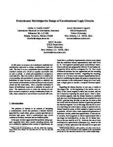
This paper discusses a new approach for Multidisciplinary Design Optimization (MDO). MDO has been a rapidly growing area of research.1-3 Thanks to these pioneering works, researchers in Computational Fluid Dynamics (CFD) are getting interested in MDO research as well. MDO research is still expanding because high fidelity CFD codes are becoming available with the aid of increasing computer power. A typical MDO problem involves competing objectives, for example in the aircraft design, minimization of aerodynamic drag, minimization of structural weight, etc. While single objective problems may have a unique optimal solution, multi-objective problems (MOPs) have a set of compromised solutions, largely known as the tradeoff surface, Pareto-optimal solutions or non-dominated solutions.4 These solutions are optimal in the sense that no other solutions in the search space are superior to them when all objectives are considered (Fig. 1). Traditional optimization methods such as the gradient-based methods5,6 are single objective optimization methods that optimize only one objective. These methods usually start with a single baseline design and use local gradient information of the objective function with respect to changes in the design variables to calculate a search direction. When these methods are applied to a MOP, the problem is transformed into a single objective optimization problem by combining multiple objectives into a single objective typically using a weighted sum method. For example, to minimize competing functions f1 and f2, these objective functions are combined into a scalar function F as (1) F = w1 ⋅ f1 + w2 ⋅ f 2 *

Professor, Institute of Fluid Science, 2-1-1 Katahira, Sendai, Japan, 980-8577, Associate Fellow AIAA Research Associate, Institute of Fluid Science, 2-1-1 Katahira, Sendai, Japan, 980-8577, Member AIAA ‡ Research Associate, 7-44-1 Jindaiji-Higashi, Chofu, Japan, 182-8522, Member AIAA †

1 American Institute of Aeronautics and Astronautics

AIAA-2005-4666 Revised Aug. 22, 2007

Feasible region G

F A

D B

E

Pareto-front C objective function f1 Figure 1 The concept of Pareto-optimality

objective function f2

objective function f2

This approach, however, can find only one of the Pareto-optimal solutions corresponding to each set of the weights w1 and w2. Therefore, one must run many optimizations by trial and error adjusting the weights to get Pareto-optimal solutions uniformly over the potential Pareto-front. This is considerably time consuming in terms of human time. What is more, there is no guarantee that uniform Pareto-optimal solutions can be obtained. For example, when this approach is applied to a MOP that has concave trade-off surface, it converges to two extreme optimums without showing any trade-off information between the objectives (Fig. 2). To overcome these difficulties, NormalBoundary Intersection Method7 and Aspiration Level Method8 were developed. An alternative approach to solve MOP is to find as many Pareto-optimal solutions as possible to reveal trade-off information among different objectives. Once such solutions are obtained, Decision Maker (DM) will be able to choose a final design with further considerations. Evolutionary Algorithms (EAs, for example, see Refs. 9 and 10) are particularly suited for this purpose. Evolutionary Algorithm is a generic name for population-based optimization methods, such as Genetic Algorithms (GAs), Evolutionary Strategies (ESs), Genetic Programming (GP), etc.11 EAs simulate the mechanism of natural evolution, where a biological population evolves over generations to adapt to an environment. Fitness, the individual, and genes in the evolutionary theory correspond to the objective function, design candidate, and design variables in design optimization problems, respectively. EAs have been extended successfully to solve MO problems.12 EAs use a population to seek optimal solutions in parallel. This feature can be extended to seek Pareto solutions in parallel without specifying weights between the objective functions. Because of this characteristic, EAs can find Pareto solutions for various problems having convex, concave and discontinuous Pareto front. The resultant Pareto solutions represent global trade-offs. In addition, EAs have other advantages such as robustness and suitability for parallel computing. Due to these advantages, EAs have been applied to MOPs very actively (EMO proceedings). EAs have been also applied to single objective and multi-objective aerospace design optimization problems.13-19

Feasible region

A

C

Pareto-front

B

objective function f1 Figure 2 Weighted-sum method applied to a MOP having a convex Pareto-front

This approach of finding many Pareto solutions works fine as it is, however, only when the number of objectives remains small (usually two, three at most, as shown in Fig. 3). To reveal trade-off information from the resultant Pareto front for real-world problems with many objectives, visualization of the Pareto front becomes an issue. Several techniques have been considered, such as parallel coordinates,20 box plot,21 and Self-Organizing Map (SOM).22 The importance of visualization of design space is also discussed in Ref. 23. Because such visualization is a tool for data mining, data mining is found very important in this approach. To support data mining activities, response surfaces are found versatile. Once the surface is constructed, it can be used for statistical analysis, for example, analysis of variance (ANOVA).24 ANOVA shows the effect of each design variables on objective functions quantitatively while SOM shows the information qualitatively. When the response surface method (RSM) is introduced for data mining as post-process of optimization, it can be applied to pre-process of optimization as a surrogate model, 25-27 too. Pre-process has been an important aspect of introduction of surrogate models because it would reduce the computational expense greatly, while it would produce rich non-dominated 2 American Institute of Aeronautics and Astronautics

AIAA-2005-4666 Revised Aug. 22, 2007

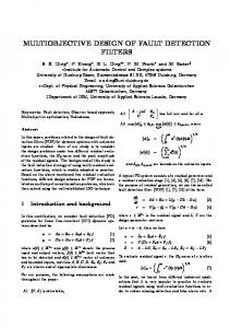
solutions efficiently. In this paper, surrogate models are introduced for both pre- and post-processes. However, it should be noted that RSM is needed for post-process primarily. EAs may be applied from the beginning in parallel to building the surrogate model. If function evaluations are very cheap, EAs may also be applied directly. As a result, the new approach for MDO named as Multi-Objective Design Exploration (MODE) can be summarized as a flowchart shown in Fig. 4. MODE is not intended to give an optimal solution. MODE reveals the structure of the design space from the trade-off information and visualizes it as a panorama for DM. DM will know the reason for trade-offs from non-dominated designs, instead of receiving an optimal design without trade-off information. The rest of the paper will explain the components of MODE used in our group, although the concept of MODE can be coupled with other RSM and optimization algorithms. Examples of data mining17,24,28 will be given briefly.

2 objectives

3 objectives

4 objectives

Projection

? Minimization problems

Figure 3 Visualization of Pareto front

Define design space

Parameterization: PARSEC, B-Spline, etc.

Choose sample points

Design of Experiment: Latin Hypercube

Construct surrogate model

Response Surface Method: Kriging Model

Find non-dominated front

Optimization: Adaptive Range Multi Objective Genetic Algorithms

Check the model and front

Uncertainty Analysis: Expected Improvement based on Kriging Model, statistics of design variables, etc.

Extract design knowledge

Data Mining: Analysis of Variance, Self-Organizing Map, etc.

Figure 4 Flowchart of Multi-Objective Design Exploration (MODE) with component algorithms

3 American Institute of Aeronautics and Astronautics

AIAA-2005-4666 Revised Aug. 22, 2007

II.

Surrogate Model

A. Kriging Model The present Kriging model expresses the unknown function y(x) as y ( x) = μ + Z ( x) (2) where x is an m-dimensional vector (m design variables), μ is a constant global model, and Z(x) represents a local deviation from the global model. In the model, the local deviation at an unknown point is expressed using stochastic processes. The sample points are interpolated with the Gaussian correlation function to estimate the distribution of the function value at the unknown point. The correlation between Z(xi) and Z(xj) is strongly related to the distance between the two corresponding points, xi and xj. In the Kriging model, a special weighted distance is used instead of the Euclidean distance because the Euclidean distance weighs all design variables equally. The distance function between the point at xi and xj is expressed as d (x i , x j ) =

m

∑θ

k

x ki − x kj

2

(3)

k =1

where θk (0≦θk≦∞) is the kth element of the parameter θ. The correlation between the point xi and xj is defined as

[

( )] = exp [− d ( x

Corr Z ( x i ), Z x The Kriging predictor27,29 is

j

i

,x j)

]

yˆ (x) = μˆ + r′R −1 (y − 1μˆ )

(4) (5)

Where μˆ is the estimated value of μ, R denotes the n×n matrix whose (i, j) entry is Corr[Z(xi), Z(xj)]. r is vector whose ith element is ri ( x) ≡ Corr Z (x), Z ( x i ) (6) 1 n and y=[y(x ),……,y(x )]. The unknown parameter, θ, for the Kriging model can be estimated by maximizing the following likelihood function: 1 n n Ln( μˆ , σˆ 2 , θ) = − ln(2π ) − ln(σˆ 2 ) − ln ( R ) 2 2 2 (7) 1 ′ −1 ˆ ˆ ( ) ( ) − y − 1 μ R y − 1 μ 2σˆ 2 where 1 denotes an m-dimensional unit vector. Maximization of the likelihood function is an m-dimensional unconstrained non-linear optimization problem. In this paper, the alternative method30 is adopted to solve this problem. For a given θ, μˆ and σˆ 2 can be defined as

[

μˆ =

σˆ 2 =

]

1′R −1 y

1′R −1 1 (y − 1 μ )′ R −1(y − 1μ )

(8) (9)

n The accuracy of the estimated value on the Kriging model largely depends on the distance from the sample points. Intuitively speaking, the closer point x is to the sample points, the more accurate yˆ (x ) is. This intuition is expressed in the mean squared error of the predictor. ⎡ (1 − 1R −1 r ) 2 ⎤ (10) s 2 (x) = σˆ 2 ⎢1 − r ′R −1 r + ⎥ 1′R −1 1 ⎥⎦ ⎢⎣ s2(x) is the mean squared error at point x, indicating the uncertainty of the estimated value.

4 American Institute of Aeronautics and Astronautics

AIAA-2005-4666 Revised Aug. 22, 2007

B. Exploration of Global Optimum and Treatment of Constraints on the Kriging model Once the approximation model is constructed, the optimum point can be explored using an arbitrary optimizer. However, there is a possibility of missing the global optimum because the estimated value includes uncertainty.

Figure 5 The objective function and the approximation model

In Fig. 5, the solid line is for the real shape of the objective function and the dotted line is for the approximation model. The minimum point on the approximation model is located near x=9, whereas, the real global minimum of the objective function is situated near x=4. Exploration of global minimum using the approximation model is apt to result in the local minimum. For a robust search of the global optimum on the approximation model, the uncertainty information is very useful.

Figure 6 The estimated value and the standard error of the Kriging model

Figure 6 shows the estimated value and the standard error (uncertainty) of the Kriging model. Around x=9.5, the standard error of the Kriging model is very small because there are many sample points around this point. Thus, the confidence interval is very short as shown in Fig. 6. On the other hand, the standard error around x=3.5 is very large due to the lack of sample points around there. Thus, the confidence interval at this point is very wide. The lower bound of this interval is smaller than current minimum on the Kriging model. Thus, it can be said that this point has some probability of being the global minimum. The probability of being the global optimum concept can be expressed by the criterion of ‘expected improvement (EI)31. In case of a minimization problem, the EI is express as follows: if y ( x) < f min = max( f min - y,0) ⎧ [ f − y ( x)] (11) I ( x) = ⎨ min 0 otherwise ⎩

E(I ) =

∫

f min

−∞

( f min − y )φ ( y ) dy

(12)

whereφis the probability density function representing uncertainty about y. By selecting the maximum EI point as additional sample points of the Kriging model iteratively, the robust exploration of the global optimum is possible. Then, if there are constraint as follows, 5 American Institute of Aeronautics and Astronautics

AIAA-2005-4666 Revised Aug. 22, 2007

ai ≤ ci ( x) ≤ bi EI subject to constraints is expressed as follows: E y ,c1 ,c2 ,......ck ( I c ) = E y (max( f min − y,0)

i = 1, L , k

(13)

b1

bk

(14)

a1

ak

∫ ⋅⋅⋅ ∫

f c1 ,...,ck y d c1 ⋅ ⋅d ck )

In order to evaluate Eq. (14), the multivariate normal distribution φ ( y, c1 ,⋅ ⋅ ⋅⋅, c k ) , which is very complicated, should be specified. Thus, in this paper, we assume that y, c1, c2, ···,ck are statistically independent in order to simplify Eq. (14). The modified Eq. (14) is as follows E y ,c1 ,L,ck ( I c ) = Ey (I ) ⋅

∏ (Φ

i =1,L, k

ci (bi ) − Φ ci ( ai )

)

(15)

= E y ( I ) ⋅ P (a1 ≤ c1 ( x) ≤ b1 ) L P (ak ≤ ck ( x) ≤ bk )

In order to calculate this value, the Kriging model is constructed for the objective function and all constraint functions separately. On the Kriging model of objective function, EI is calculated, and on the Kriging models of constraints, the probability to satisfying each constraint is calculated. Based on these values, the next additional point for balanced local and global search is selected, while satisfying the constraints.

III.

Adaptive Range Multi-Objective Genetic Algorithms

Pareto solutions and Pareto front are exact solutions by definition. Because it is difficult to show that numerical solutions are exact, numerical solutions and the corresponding front are usually called as non-dominated solutions and non-dominated front, respectively. They are non-dominated among the solutions generated by the computation (Fig. 7). Except for the introduction of range adaptation operator, the present ARMOGAs’ operators15 are the same as the MOEAs.9 Therefore, each genetic operator of the MOEAs adopted here is firstly explained. Then the unique procedure of ARMOGAs is described in this chapter.

Pareto front (exact) Approximate Pareto front Pareto solutions (exact) Extreme Pareto solutions (exact) Non-dominated solutions (numerical) Non-dominated front (numerical)

Utopia

Figure 7 Definition of Pareto solutions and non-dominated solutions

6 American Institute of Aeronautics and Astronautics

AIAA-2005-4666 Revised Aug. 22, 2007

A. Algorithm of Multi-Objective Evolutionary Algorithms 1. Binary and Floating-Point Representation As GAs originally simulated natural evolution, binary numbers were often used to represent design parameter values. However, for real function optimizations, such as aerodynamic optimization problems, it is more straightforward to use real numbers. Thus, the floating-point representation is adopted here. 2. Coding and Decoding GAs require both phenotype and genotype design variables. The phenotype design variable represents the actual design variables, such as length, angle, shape, etc. On the other hand, the genotype design variable is a binary number (Binary GAs) or a real number in [0,1] (Real-coded GAs). The operators of many GAs require genotype representation of design parameters. Therefore, actual design variables (phenotype representation) must be converted to the genotype representation. The conversion from phenotype to genotype is called “coding,” and conversely, the conversion from genotype to phenotype is “encoding.” For real-parameter design problems, such as aerodynamic optimizations, it is not favorable to use binary representation. One reason for this is that phenotype design space is not continuous by binary representation. For the present floating-point representation, i-th design parameter pi is coded to genotype value ri, which is normalized in [0,1]: pi − pi , min ri = (16) pi , max − pi , min 3. Initial Population The results of GAs can be affected by the initial population if the number of individuals per generation is small. It would be better to generate initial individuals in a wide range of design spaces. Here, the initial population is generated randomly. 4. Evaluation As GAs use only objective-function values for optimization, no modification of evaluation tools is required. In addition, it is easy to apply Master-Slave type parallelization systems to conserve computational resources because GAs do not have to compute design candidates sequentially, unlike gradient-based method. 5. Selection GAs choose superior individuals as parents to generate new design candidates. Therefore, selection has a large influence on search performance of GAs. For single-objective optimizations, as the aim is to obtain the best solution, selection is based on the fitness value given by the objective-function value. However, Pareto-optimal solutions must be obtained for MO optimization. To obtain Pareto solutions effectively, each individual is assigned a rank based on the Pareto ranking method and fitness sharing. In the present MOEAs, Fleming and Fonseca’s Paretoranking method12 is adopted. Each individual is assigned a rank according to the number of individuals dominating it, as shown in Fig. 8. The fitness value (Fi) of individual i is assigned based on the following equation: Fi = N −

∑

Ri −1 k =1

μ (k ) − 0.5(μ ( Ri ) − 1)

(17)

where N is the number of solutions, and μ(Ri) is the number of solutions in rank Ri. Thereafter, the standard sharing approach is adopted to prevent choosing similar solutions as parents and to maintain diversity of the population. The assigned fitness values are divided by the niche count: F (18) Fi′ = i nci Here, niche count nci is calculated by summing the sharing function values: nci = ∑ j =1 sh(d ij ) N

⎛ ⎛ d ij ⎜1 − ⎜ sh(d ij ) = ⎜ ⎜⎝ σ share ⎜⎜ ⎝0

⎞ ⎟⎟ ⎠

(19)

α

d ij < σ share others

7 American Institute of Aeronautics and Astronautics

(20)

AIAA-2005-4666 Revised Aug. 22, 2007

⎛ f ki − f k j ⎜⎜ ∑ k =1 ⎝ u k − l k M

d ij =

⎞ ⎟⎟ ⎠

(21) where uk is the maximum objective-function value of k at the present generation, lk is the minimum objectivefunction value of k at the present generation, and α is the sharing function parameter. If the distance between individuals i and j is lower than σshare, then niche count increases to reduce the fitness of the solution. The normalized niching parameter σshare is proposed as follows:

(1 + σ share )M − 1 = N (σ share )M

(22) where N is the size of the population and M is the number of objective functions. After shared fitness values are determined for all individuals, the stochastic universal selection (SUS) is applied to select better solutions for producing a new generation. Unlike roulette wheel selection method, only one random number is chosen for the whole selection process for SUS. As many different solutions should be chosen to maintain the diversity, a set of N equi-spaced numbers is created.

f2

1 6 3 1

4

1 1 f1 Figure 8 Pareto ranking method (Rank 1 means non-dominated solutions)

6. Crossover Crossover is an operator that interchanges the genotype parameters of selected parents and produces two different design candidates. Probability of crossovers and crossover method markedly affect the search performance of GAs. For the binary representation, crossover interchanges the bit strings of selected parents. However, many crossover methods have been proposed for real-parameter GAs. Simulated binary crossover (SBX) operator9 creates offspring based on the distance between the parents. If the two parents are closely related to each other, SBX is likely to generate new offspring near the parents. On the other hand, if the two parents are more distantly related, it is possible for solutions to be created away from the parents. This operator is described as follows: (23a) Child1 = 0.5 [(1+βq)⋅Parent1 + (1–βq)⋅Parent2 ] (23b) Child2 = 0.5 [ (1–βq)⋅Parent1 + (1+βq)⋅Parent2 ]

⎧(2 ⋅ ran1)1 (ηc +1) ⎪ 1 (η c +1) β q = ⎨⎛ ⎞ 1 ⎟⎟ ⎪⎜⎜ ⎩⎝ 2 ⋅ (1 − ran1) ⎠

(23c)

7. Mutation Mutation maintains diversity and expands the search space by changing the design parameters. If the mutation rate is high, a GA search is close to a random search and results in slow convergence. Therefore, an adequate value is required for the mutation rate. For binary representation, mutation is performed to reverse the bit strings. It is not as simple for real-coded GAs as for binary GAs. This is realised by adding disturbances to the design parameters.

8 American Institute of Aeronautics and Astronautics

AIAA-2005-4666 Revised Aug. 22, 2007

Polynomial mutation, which is similar to the SBX operator described in previous section, has been proposed9: (24) Childmutation = Childcrossover + (xmax–xmin)⋅δ where δ is calculated from the polynomial probability distribution:

⎧⎪(2 ⋅ ran 2 )1 (η m +1) − 1 ⎪⎩1 − 2 ⋅ (1 − ran 2)1 (η m +1)

δ =⎨

[

]

(25) where ran2 is a uniform random number in [0,1]. A value of ηm determines the perturbation size of mutation. 8. Archiving To obtain Pareto solutions efficiently, it would be better to include past excellent solutions as current solutions. In the present MOEAs, two archiving techniques are combined. The first is the Best-xN technique, which keeps the latest better solutions and parent generation of (x-1)N size and uses these solutions for the selection process. The second is the standard archiving technique, which is comprised of all previous solutions to prevent the loss of previous excellent solutions. These two methods are combined in the present MOEAs as shown in Fig. 9. The procedure is as follows: 1. Fitness values based on the fitness assignment operators are assigned to the present population and the Best-xN group. Here, x is set to 2. 2. According to the fitness value, the top N individuals are chosen for the next step. In addition, the top (x-1)N individuals are preserved as the Best-xN group. 3. Fitness values are assigned to chosen N individuals. 4. SUS is used to select the parents. Then, crossover and mutation are applied to generate new individuals. 5. Several individuals from the Best-xN group are replaced by the same number of individuals from the archives. Best-xN [(x-1)N individuals]

Better individuals

Archiving (all solutions)

Present population [N individuals]

Fitness assignment [xN individuals] Selection for top N population Fitness assignment [N individuals] Selection for mating pool Crossover and mutation

Figure 9 Archiving procedure used in the present MOEAs

9. Constraint-Handling Technique In many real-world problems, it is common to have several constraints. Many constraint-handling techniques have been proposed, however, it is not easy for GAs to solve constrained-problems compared to gradient-based methods. A popular and easy constraint-handling strategy is the penalty function approach in which a penalty value is added to the objective-function value if the design violates the constraint. Although several penalty functions have been proposed, it is difficult to choose appropriate penalty values a priori. In the present MOEAs, an extended Pareto ranking method based on constraint-dominance is used. Constraintdominance is defined as follows9: A solution xi is said to ‘constrain-dominate’ a solution xj, if any of the following conditions are true: 1. xi is feasible and xj is not. 9 American Institute of Aeronautics and Astronautics

AIAA-2005-4666 Revised Aug. 22, 2007

2. xi and xj are both infeasible, but xi has a smaller constraint violation. 3. xi and xj are feasible and xi dominates xj in the usual sense. Figure 10 shows the example of a Pareto ranking method based on constraint-dominance for the two-objective minimization problem with one constraint. Based on this approach, it would be easy to generate new offspring that satisfy the constraints because feasible solutions are likely to be chosen as the parents. However, it is possible for good solutions to lie close to the edge of the feasible and infeasible region in many industrial problems. Therefore, an adequate tolerance of the constraint (ctol) should be introduced to the constraint violation: G – ctol ≤ 0 (26) where G is an original constraint less than zero. As the tolerance ctol is introduced, solutions having smaller violation than ctol are assumed to be feasible for constraint-dominance. This enables EAs to search for solutions near the boundary between feasible and infeasible solutions. To consider the aerodynamic optimization using time-consuming CFD, it is unfavorable to generate many violated candidates. If it is possible to determine that the solution violates constraints before CFD computation, such as geometrical constraints (length, angle, etc.), it is possible to prevent generating such solutions, as it would be a waste of computation time in CFD. In the case of aerodynamic optimization, it would be better to take account of the above problem.

f2

Constraint 7 1 6 8 Infeasible

4 2 Feasible

1

1

f1 Pareto front Figure 10 Example of constrain-dominance.

B. Algorithm of Adaptive Range Multi-Objective Genetic Algorithms To reduce the large computational burden, the reduction of the total number of evaluations is needed. On the other hand, a large string length is necessary for real parameter problems. Oyama developed real-coded ARGAs and applied them to the transonic wing optimization.14 According to the encoding system based on normal distribution (Fig. 11) built by population statistics consisting of better designs computed before, ARGAs can find a good optimal design efficiently. The basis of ARMOGAs is the same as ARGAs, but a straightforward extension may cause a problem in the diversity of the population. Therefore, ARMOGAs have been developed based on ARGAs to deal with multiple Pareto solutions for the multi-objective optimization. In addition, archiving and constraint-handling techniques are considered to select better solutions to decide new search range. This section describes genetic operators of ARMOGAs. ARMOGAs differ from MOEAs described above with regard to the application of range adaptation. Therefore, before starting range adaptation, the MOEAs and ARMOGAs in the present study are identical. A flowchart of ARMOGAs is shown in Fig. 12. The range adaptation starts at Msa generation and is carried out every Mra generations. The new decision space is determined based on the statistics of selected better solutions, and then the new population is generated in the new decision space. Thereafter, all the genetic operators are applied to the new design space. ARMOGAs are able to find Pareto solutions more efficiently than conventional MOEAs because of the concentrated search of the promising design space out of the large, initial design space. ARMOGAs can adapt their

10 American Institute of Aeronautics and Astronautics

AIAA-2005-4666 Revised Aug. 22, 2007

search region as shown in Fig. 13. In contrast, the search region of conventional EAs remains unchanged. The encoding system is based on the normal distribution with the plateau region as shown in Fig. 14. The selected designs locate in the plateau region, and the normal distribution region is determined based on the population statistics to better preserve the diversity of solution candidates. Re-initialization helps to maintain the population diversity. Probability

ri

−∞

0

pn,i

pi=μi

+∞

xi

pi

Figure 11 Normal distribution for encoding in real-coded ARGAs

Initial population Evaluation Termination criteria

Selection

Archive

Sampling

Crossover

Range adaptation

Mutation

Re-initialisation

Figure 12 Flowchart of ARMOGAs

Superior solution Search region

Inferior solution Search region Probability

Probability

x x1L

x1U

(a) Conventional MOEAs

x x1L

x1U

(b) ARMOGAs

Figure 13 Sketch of search region

11 American Institute of Aeronautics and Astronautics

AIAA-2005-4666 Revised Aug. 22, 2007

1−αr ≤ ri ≤ 1

Probability

0 ≤ ri ≤ αr I

pi,min

II

αr < ri < 1−αr μi

μi−fli

III

μi+fli

pi pi,max

Figure 14 Sketch of probability distribution of phenotype design variable pi in ARMOGAs

1. Sampling for Range Adaptation Range adaptation needs to select superior solutions to determine the new design space based on the statistics. The solutions, which have higher fitness values based on Pareto ranking method, are selected to determine the reasonable search range. It would be better to select many solutions to prevent the creation of new search regions that do not include the global optimum. On the other hand, many solutions for range adaptation generally interfere with the decrease in size of the search space. The solutions are selected at random according to their fitness given by the following solution sets: 1. PRnon% non-dominated solutions from all solutions. (PRnon=100) 2. PRarc% solutions from the archive. (PRarc=0) 3. PRprs% solutions from the latest generation. (PRprs=0) 4. PRvio% solutions that violate the constraint. (PRvio=1, at least one design) Solution set 4 is introduced to search near the boundary between feasible and infeasible solutions, as the globaloptimum for constraint problems is often located there. According to the amount of violation, violated designs are sampled. The probabilities in bracket are used in this optimization. In this case, only non-dominated solutions with several infeasible designs are selected to determine new design range. 2. Range Adaptatoin In the ARMOGAs, the search region is changed according to the population statistics of the average and the standard deviation. The range adaptation adopts the Normal distribution to search global solutions efficiently. Figure 11 shows the Normal distribution used for encoding in the real-coded ARGAs. The real value of the i-th design variable pi is encoded to a real number ri defined in (0,1) such that ri is equal to the integrations of the normal distribution from -∞ to pn,i: ri =

∫

pn , i

−∞

p n,i =

N (0,1)( z ) dz

pi − μ i

(27a) (27b)

σi where μi is the average of the i-th design variable, and σi is the standard deviation of the i-th design variable.

The basic idea of encoding system in ARMOGAs is the same as for real-coded ARGAs, but a straightforward extension is not suitable in diversity of the population. To better preserve the diversity of solution candidates, the Normal distribution for encoding has to be changed. Figure 14 shows the search range with the distribution of probability. The search region is partitioned into three parts, I, II, and III. Regions I and III make use of the same encoding method as ARGAs. The real value of the i-th design variable Pi is encoded to a real number ri defined in (0,1). In contrast, region II adopts the conventional realnumber encoding method. The plateau region (region II) is defined by the upper and lower design variables of chosen solutions. Then, the normal distribution is considered at both sides of the plateau determined by the average (μi) and the standard deviation (σi). This encoding system is controlled by the parameters αr and fli, where αr (