Efficient Design Space Exploration for Application Specific Systems-on-a-Chip Giuseppe Ascia a , Vincenzo Catania a , Alessandro G. Di Nuovo a,∗ , Maurizio Palesi a , Davide Patti a a Dipartimento
di Ingegneria Informatica e delle Telecomunicazioni Universit`a di Catania, Viale A. Doria 6, 95125 Catania, Italy
Abstract A reduction in the time-to-market has led to widespread use of pre-designed parametric architectural solutions known as system-on-a-chip (SoC) platforms. A system designer has to configure the platform in such a way as to optimize it for the execution of a specific application. Very frequently, however, the space of possible configurations that can be mapped onto a SoC platform is huge and the computational effort needed to evaluate a single system configuration can be very costly. In this paper we propose an approach which tackles the problem of design space exploration (DSE) in both of the fronts of the reduction of the number of system configurations to be simulated and the reduction of the time required to evaluate (i.e., simulate) a system configuration. More precisely, we propose the use of Multi-objective Evolutionary Algorithms as optimization technique and Fuzzy Systems for the estimation of the performance indexes to be optimized. The proposed approach is applied on a highly parameterized SoC platform based on a parameterized VLIW processor and a parameterized memory hierarchy for the optimization of performance and power dissipation. The approach is evaluated in terms of both accuracy and efficiency and compared with several established DSE approaches. The results obtained for a set of multimedia applications show an improvement in both accuracy and exploration time. Key words: Design Space Exploration, Multiobjective Optimization, Embedded System Design, Very Long Instruction Word Processor, Fuzzy Estimation, Evolutionary Computation
∗ Corresponding Author Email addresses:
[email protected] (Giuseppe Ascia),
[email protected] (Vincenzo Catania),
[email protected] (Alessandro G. Di Nuovo),
[email protected] (Maurizio Palesi),
[email protected] (Davide Patti).
Preprint submitted to Journal of System Architecture
21 December 2006
1 Introduction
The design flow of a SoC features the combined use of heterogeneous techniques, methodologies and tools with which an architectural template is gradually refined step by step on the basis of functional specifications and system requirements. Each phase in the design flow can be considered as an optimization problem which is resolved by defining and/or setting some of the system’s free parameters in such a way as to optimize certain performance indexes. These optimization problems are usually tackled by means of processes based on successive cyclic refinements: starting from an initial system configuration, they introduce transformations at each iteration in order to enhance its quality. In this paper we focus on Platform-based design. In particular we refer to a design flow based on parameterized SoC platforms. With the term “platform” we intend a coordinated family of hardware-software architectures developed to promote high levels of re-use of hardware and software components in the rapid, low-risk design of application-oriented derivative products. These could take the form of a SoC or more complex electronic systems, and the platforms will be offered by a number of different vendors working in various product application domains, in the form of both relatively fixed platforms and ones incorporating reconfigurability. The apparent rigidity of a platform, due to a fixed architecture, is made flexible by means of a high degree of programmability and great parameterizations of the modules it contains [1]. Variations in parameters have a considerable impact on the performance indexes being optimized (such as performance, power consumption, area, etc.). Defining strategies to ”tune” parameters so as to establish the optimal configuration for a system is a challenge known as Design Space Exploration (DSE). Obviously, it is computationally unfeasible to use an exhaustive exploration strategy. The size of the design space grows as the product of the cardinalities of the variation sets for each parameter. In addition, evaluation of a single configuration almost always requires the use of simulators or analytical models which are often highly complex. Another problem is that the objectives being optimized are often conflicting. The result of the exploration will therefore not be a single solution but a set of tradeoffs which make up the Pareto set. Any DSE technique can be schematically represented as in Figure 1. Starting with a base configuration, the exploration process is an iterative refinement process comprising two main stages: evaluation and tuning of the parameters of the configuration. The evaluation phase often boils down to a system-level simulation which constitutes a bottleneck in the exploration process. The tuning phase uses the results of the evaluation phase to modify the system configuration parameters so as to optimize certain performance indexes. The cycle ends when a system configuration that meets the design constraints has been obtained, or, more frequently, when a set of Pareto-optimal configurations for the indexes to be optimized have been accumulated.
2
Fig. 1. General design space exploration flow.
The main objective of a design space exploration strategy is to minimize the exploration time while guaranteeing good-quality solutions. Most contribution to DSE to be found in literature address the problem in two complementary ways either by minimizing the number or configurations visited (i.e., simulated), or by minimizing the time required to evaluate (i.e., simulate) the system configurations visited (see Figure 2). Works [2–4] belong to the first category. In [2] Givargis et al. propose an exact technique based on the notion of dependence between parameters. The basic idea of their approach is to cluster dependent parameters and then carry out an exhaustive exploration within these clusters. If the size of these clusters increases too much due to great dependency between the parameters, the approach becomes a purely exhaustive search, with a consequent loss of efficiency. To deal with these problems approximate approaches have been proposed in literature which further reduce the exploration space but give no guarantee that the solutions found will be optimal. Fornaciari et al. in [3] use sensitivity analysis to reduce the space of exploration from the product of the cardinalities of the sets of variation of the parameters to their sum. This approach can be seen as a simplified version of [2], as all the parameters are considered to be independent. In this way exploration is carried out by fixing the less sensitive parameters and varying the most sensitive parameter until the objective is optimized. Another approximate approach was proposed by Ascia et al. in [4]. They propose the use of multi-objective genetic algorithms as
Fig. 2. Design space exploration approaches.
3
optimization technique for DSE. Other DSE approaches which perform the pruning of the design space con be found in [5–8]. Most of the approaches belonging to the second category are of limited applicability and not general (or scalable) since they are often tailored for a specific system architecture. The use of an analytical model to speed up evaluation of a system configuration is presented in [9]. Statistical simulation is used in [10] to enable quick and accurate design decisions in the early stages of computer design, at the processor and system levels. A recent approach [11] uses statistical simulation to speed up the evaluation of configurations by a multi-objective genetic algorithm. In this paper we propose an approach which tackles the problem on two fronts: the prune of the design space and the reduction of the time required to evaluate system configurations. To achieve this, we propose the use of a Genetic Fuzzy System to increase efficiency or, with the same level of efficiency, improve the accuracy of any DSE strategy. We propose the use of a genetic algorithm as exploration heuristic and a fuzzy system as an evaluation tool. The methodology proposed is applied to the exploration of the design space of a parameterized SoC platform based on a VLIW processor. The use of such platforms for the development of advanced applications, above all in the mobile multimedia area is a representative testbed to evaluate the methodology proposed. The high degree of parametrization that these platforms feature, combined with the heterogeneous nature of the parameters being investigated, both hardware (architectural, micro-architectural and technology-dependent parameters) and software (compilation strategies and application parameters), demonstrates the scalability of the approach. The rest of the paper is organized as follows. A formal statement of the problem is given in section 2. Section 3 outlines some of contributions representing the state of the art of DSE techniques proposed in the literature. Section 4 gives a general description of our proposal. Section 5 present the simulation framework and the quality measures we used to assess and compare the performances of the proposed algorithm. In Section 6 the methodology is applied to real case studies and compared, in terms of both efficiency and accuracy, with methodologies presented in Section 3. Finally Section 7 summarizes our contribution and outlines some directions for future work.
2 Formulation of the Problem
Although the methodology we propose is applied to and evaluated on a specific case study (optimization of a highly parameterized VLIW-based SoC platform), it is widely applicable. For this reason, in this section we will provide a general formulation of Design Space Exploration problem. Let S be a parameterized system with n parameters. The generic parameter pi , i ∈ 4
{1, 2, . . . , n} can take any value in the set Vi . A configuration c of the system S is a n-tuple hv1 , v2 , . . . , vn i in which vi ∈ Vi is the value fixed for the parameter pi . The configuration space (or design space) of S [which we will indicate as C(S)] is the complete range of possible configurations [C(S) = V1 × V2 × . . . × Vn ]. Naturally not all the configurations of C(S) can really be mapped on S. We will call the set of configurations that can be physically mapped on S the feasible configuration space of S [and indicate it as C ∗ (S)]. Let m be the number of objectives to be optimized (e.g. power, cost, performance, etc.). An evaluation function E : C ∗ (S) × B −→ ℜm is a function that associates each feasible configuration of S with an m-tuple of values corresponding to the objectives to be optimized when any application belonging to the set of benchmarks B is executed. Given a system S, an application b ∈ B and two configurations c′ , c′′ ∈ C ∗ (S), c′ is said to dominate (or eclipse) c′′ , and is indicated as c′ ≻ c′′ , if given o′ = E(c′ , b) and o′′ = E(c′′ , b) it results that o′ ≤ o′′ and o′ 6= o′′ . Where vector comparisons are interpreted component-wise and are true only if all of the individual comparisons are true (o′i ≤ o′′i ∀ i = 1, 2, . . . , m). The Pareto-optimal set of S for the application b is the set: P(S, b) = {c ∈ C ∗ (S) : ∄ c′ ∈ C ∗ (S), c′ ≻ c} that is, the set of configurations c ∈ C ∗ (S) not dominated by any other configuration. Pareto-optimal configurations are configurations belonging to the Paretooptimal set and the Pareto-optimal front is the image of the Pareto-optimal configurations, i.e. the set: PF (S, b) = {o : o = E(c, b), c ∈ P(S, b)} The aim of the paper is to define a Design Space Exploration (DSE) strategy that will give a good approximation of the Pareto-optimal front for a system S and an application b, simulating as few configurations as possible.
3 Design Space Exploration Approaches
In this section we will present and discuss three approaches to DSE. The first, GA, uses Genetic Algorithms as the optimization engine. A configuration is mapped onto a chromosome and a population of configurations is made to evolve until it converges on the Pareto-optimal set. The second approach, PBSA (Pareto Based Sensitivity Analysis), uses sensitivity analysis to order the parameters by importance. Each parameter is thus made to vary independently of the others, the imme5
diate consequence being the need to visit a number of configurations, which grow in a linear fashion as the number of parameters increases (rather than exponentially as happens in an exhaustive analysis). The third, DEP (short for DEPendency analysis), is an exact approach. It uses parameter dependence information to divide the configuration space up into subspaces of a size that will enable an exhaustive search to be made. The following subsection will give a detailed description of these approaches, concluding each one with a list of their strong and weak points.
3.1
Genetic-based Approach
In general, when the configuration space is too large for exhaustive exploration, the use of evolutionary techniques represents an alternative solution. Genetic algorithms (GAs) have been applied in various VLSI design environments [12], for example in layout problems such as partitioning [13], placement [14] and routing [15]; in design problems such as power estimation [16], technology mapping [17] and netlist partitioning [18]; and in reliable chip testing through efficient test vector generation [19]. All these problems are untractable in the sense that no polynomial time algorithm can guarantee an optimal solution and they actually belong to the NP-complete and NP-hard categories. The GA-based approach is highly suitable for a general, efficient solution to these problems. It is a general approach because the GA solution to a problem only requires the definition of a representation of the configuration, the genetic operators and the objective functions to be optimized. In addition, it does not require detailed knowledge of the system, for example the internal architecture or parameter dependency, if any, unlike DEP. We applied GAs for the design space exploration of parameterized systems based on both RISC processor [20,21] and VLIW processor [4]. Strengths. The approach is a general one and its application does not require detailed knowledge of the system. The only thing that needs to be defined is the mapping of a system configuration onto a chromosome. The most simple way to do this is to use a gene for each system parameter and limit their range of variation to that of the parameters they represent. Weaknesses. Unlike DEP, a GA-based approach is an approximate one. This means that the set of solutions found is not the Pareto-optimal set but an approximation of it. 6
3.2
Pareto Based Sensitivity Analysis
The Pareto-Based Sensitivity Analysis (PBSA) is a generalization of the sensitivity analysis approach proposed by Fornaciari et al. in [3]. In its basic formulation, sensitivity analysis is a mono-objective approach in the sense that it provides one and only one solution that optimizes a certain objective function. This objective function may be expressed as a combination of several objective functions (in [22,3], for example, it is expressed as the power-delay product for a memory hierarchy). Sensitivity analysis reduces the space of possible configurations in two phases. The aim of the first phase is to identify the parameters which most influence the objective function to be optimized—the sensitivity analysis phase. For a system with n parameters, determination of the degree of sensitivity of each parameter consists of fixing n − 1 parameters and varying one of them, determining the maximum range of variation of the objective function. The set of parameters that do not reach a user defined sensitivity threshold can be ignored at the purpose of the exploration. The next phase, design space exploration phase, identifies the optimal value for each parameter, from the most to the least sensitive. The number of configurations to Q P be evaluated goes down from ni=1 |Vi | to ni=1 |Vi |. To overcome the limits of the mono-objective approach described, in [23] we defined a new technique based on sensitivity analysis to perform multi-objective optimization based on the notion of Pareto optimum. Strengths. As in GA, the PBSA application does not require detailed knowledge of the system. The user can also establish the accuracy/efficiency tradeoff by acting on the value of the threshold. A low threshold value means considering more parameters. This leads to an increase in the configuration space (and therefore the time required to explore it) but consequently to an improvement in terms of the accuracy of the solutions found. Vice versa, using a high threshold value means that only the most sensitive parameters are considered, thus limiting the space of exploration but reducing the accuracy of the solutions. Weaknesses. This approach is an approximate one and the quality of the solutions found depends on the threshold value. However, once a threshold value has been set, the number of parameters exceeding it depends on the application involved. A threshold value that gives excellent results in terms of accuracy and/or efficiency for one application may not do so for another.
3.3
Dependency Approach
The dependency approach (DEP) was proposed by Givargis et al. in [2]. The basic idea is to exploit information regarding the dependency of certain parameters of the system being examined in order to reduce the dimensions of the exploration space. 7
Parameter dependency is captured by an oriented graph (dependency graph), in which nodes represent parameters and oriented arcs represent dependency between two nodes (parameters). A path from a node A to a node B indicates that the Pareto-optimal configurations of B only have to be calculated after the Pareto-optimal configurations of all the nodes on the path connecting A to B have been calculated. During calculation, all the parameters that are not on the path connecting A and B can be set to an arbitrary value. The exploration algorithm operates on the dependency graph in two phases. The first phase is a local search for the Pareto-optimal configurations and can be further divided into two sub-phases. The first clusters the parameters in relation to their degree of dependency, while the second performs an exhaustive exploration of the subspace of configurations generated by each cluster to obtain the Pareto-optimal configurations. The second phase of the algorithm combines the clusters two by two and extracts their Pareto-optimal configurations. This is repeated until all the clusters have been combined. Strengths. The dependency approach is an exact approach in the sense that if the dependency graph is correct it is possible to obtain all the Pareto-optimal configurations. Weaknesses. Application of the method requires detailed knowledge of the system in order to plot the dependency graph. In [2] the authors suggest that when the dependency between two parameters is uncertain, the conservative choice is to consider them as being dependent. The problem is that by doing so there is a possibility of generating cluster containing such a large number of parameters that the associated configuration space is too large to be explored exhaustively. Another weak point is the scalability of the approach as the complexity of the system increases: if the parameters are highly interdependent the approach may become inapplicable.
4 The Genetic Fuzzy Approach for Design Space Exploration
Unfortunately, the approaches introduced in the previous section may be expensive (sometimes computationally infeasible) when a single simulation (i.e., the evaluation of a single system configuration) requires a long compilation and/or execution time. For the sake of example, referring to the computer system architecture considered in this paper, Table 1 reports the computation effort needed for one evaluation (i.e. simulation) of just a single system configuration for several media and digital signal processing application benchmarks. By a little multiplication we can notice that a few thousands of simulations (just a drop in the immense ocean of feasible configurations) could last from a day to weeks! 8
Table 1 Evaluation time for a simulation (compilation + execution) for several multimedia benchmarks on a Pentium IV Xeon 2.8 GHz Linux Workstation. Benchmark Description Input size Evaluation time (KB)
(sec)
625
5.4
wave
Audio Wavefront computation
g721-enc
CCITT G.711, G.721 and G.723 voice compressions
8
25.9
jpeg-codec
jpeg compression and decompression
32
33.2
mpeg2-dec
MPEG-2 video decoding
400
143.7
adpcm-enc
Adaptive Differential Pulse Code Modulation speech encoding
295
22.6
adpcm-dec
Adaptive Differential Pulse Code Modulation speech decoding
16
20.2
fir
FIR filter
64
9.1
The primary goal of this work was to create a new approach which could run as few simulations as possible without affecting the good performance of the GA approach. For this reason we developed an intelligent GA approach which has the ability to avoid the simulation of configurations that it foresees to be not good enough to belong the Pareto-set and to give them fitness values according to a fast estimation of the objectives. This feature was implemented using a Fuzzy System (FS) to approximate the unknown function from configuration space to objective space. The approach could be briefly described as follows: the GA evolves normally; in the meanwhile the FS learns from simulations until it becomes expert and reliable. From this moment on the GA stops launching simulations and uses the FS to estimate the objectives. Only if the estimated objective values are good enough to enter the Pareto-set will the associated configuration be simulated. We chose a fuzzy rule-based system as an estimator above all because it has cheap additional computational time requirements for the learning process, which are negligible as compared with simulation time. A further advantage of the system of fuzzy rules is that these rules can be easily interpreted by the designer. The rules obtained can thus be used to for detailed analysis of the dynamics of the system. The basic idea of our methodology is depicted in Figure 3. The qualitative graph shows the exploration time versus the number of system configurations evaluated. If we consider a constant simulation time, the exploration time grows linearly with the number of system configurations to be visited. Our proposal is to use an estimator 9
Fig. 3. Saving in exploration time achieved by using the proposed approach.
which learns during the initial phase of the exploration (training phase). When the estimator becomes reliable, the simulator engine is turned off and the exploration continues by using the estimator in place of the simulator. Since the evaluation of a system configuration carried out by a simulator is generally much more time consuming as compared to the evaluation carried out by the estimator, the saving in terms of computation time increase with the number of system configurations to be explored. More precisely, in the training phase the estimator is not reliable and the system configurations are evaluated by means of a simulator which represents the bottleneck of the DSE. The actual results are then used to train the estimator. This cycle continues until the estimator becomes reliable. From that point on, the system configurations are evaluated by the estimator. If the estimated results are predicted to belong the Pareto set, the simulation is performed. This avoid the insertion in the Pareto set of non-Pareto system configurations. Algorithm 1 Evaluation of a configuration. Require: c ∈ C (Configuration Space) Ensure: power, ex time if F easible(c) = true then ConfigurePlatform(c) results = RunSimulation() power = PowerEstimation(results) ex time = ExTimeEstimation(results) else power = ex time = ∞ end if
10
Algorithm 2 RunSimulation(). if FuzzyEstimatorReliable() == true then results = FuzzyEstimation(c) if IsGoodForPareto(results) == true then results = SimulatePlatform(c) FuzzyEstimatorLearn(c, results) end if else results = SimulatePlatform(c) FuzzyEstimatorLearn(c, results) end if Algorithms 1 and 2 explain how the proposed approach evaluates a configuration suggested by the GA. The reliability condition is essential in this flow. It assures that the estimator is reliable and that it can be used in place of the simulator. The reliability test can be performed in several way as follows: (1) The estimator is considered to be reliable after a given number of samples have been presented. In this case the duration of the training phase is constant and user defined. (2) During the training phase the difference between the actual system output and the predicted (approximated) system output is evaluated. If this difference (error) is below a user defined threshold, the estimator is considered to be reliable. (3) The reliability test is performed using a combination of criteria 1 and 2. That is: During the training phase the difference between the actual system output and the predicted (approximated) system output is evaluated. If this difference (error) is below a user defined threshold and a minimum number of samples have been presented, the estimator is considered to be reliable. The first reliability test is suitable only when the function to approximate is known a priori, so it is possible to preset the number of samples needed by the estimator before the GA exploration starts. In our application the function is obviously not know, so the second test appear to be more suitable. However the design space is wide, for this reason we expect that the error measure oscillates for early evaluations and it will be reliable only when a representative set of system configurations were visited, i.e. a minimum number of configurations were evaluated. So the third test is the one which meets our requirements. 4.1
Our Implementation of Multi-Objective Genetic Algorithm
For this work we chose SPEA2 [24], which is very effective in sampling from along the entire Pareto-optimal surface and distributing the solutions generated over the trade-off surface. SPEA2 is an elitist multi-objective evolutionary algorithm 11
which incorporates a fine-grained fitness assignment strategy, a density estimation technique, and an enhanced archive truncation method.
Fig. 4. Mapping of a system configuration into a chromosome.
The representation of a system configuration is on a chromosome whose genes define the parameters of the system. The chromosome of the GA will then be defined with as many genes as there are free parameters and each gene will be coded according to the set of values it can take. For instance Figure 4 shows our reference parameterized architectures and its mapping on the chromosome. Crossover (recombination) and mutation operators produce the offspring. In our specific case, the mutation operator randomly modifies the value of a parameter chosen at random. The crossover between two configuration exchanges the value of two parameters chosen at random. Application of these operators may generate non-valid configurations (i.e. ones that cannot be mapped on the system). Although it is possible to define the operators in such a way that they will always give feasible configurations, or to define recovery functions, these have not been taken into consideration in the paper. Any unfeasible configurations are filtered by the feasible function. A feasible function fF : C −→ {true, f alse} assigns a generic configuration c belonging to the configuration space C a value of true if it is feasible and f alse if c cannot be mapped onto the parameterized system. A stop criterion based on convergence makes it possible to stop iterations when there is no longer any appreciable improvement in the Pareto sets found. The convergence criterion we propose uses the function of coverage [25] between two sets to establish when the GA has reached convergence.
4.2
Fuzzy Function Approximation
In our approach we used the well-known Wang and Mendel method [26], which consists of five steps: • Step 1 Divides the input and output space of the given numerical data into fuzzy regions. • Step 2 Generates fuzzy rules from the given data. 12
Fig. 5. Fuzzy Rule Generation Example.
• Step 3 Assigns a degree to each of the generated rules for the purpose of resolving conflicts among them (rule with higher degree wins). • Step 4 Creates a combined fuzzy rule base based on both the generated rules and, if there were any, linguistic rules previously provided by human experts. • Step 5 Determines a mapping from the input space to the output space based on the combined fuzzy rule base using a defuzzifying procedure. From Step 1 to 5 it is evident that this method is simple and straightforward, in the sense that it is a one-pass buildup procedure that does not require time-consuming training. In our implementation the output space could not be divided in Step 1, because we had no information about boundaries. For this reason we used Takagi-Sugeno fuzzy rules [27], which have as consequents a real number sj associated with all the M outputs: if x1 is S1 and . . . and xN is SN then y1 = s1 , . . . , ym = sM where Si are the fuzzy sets associated with the N inputs. In this work we chose to use the maximum granularity to describe the features, i.e. the number of fuzzy sets are equal to the number of degrees of freedom for each input variable. For this reason Step 3 was not necessary. Steps 2 and 4 were iterated with the GA: after every evaluation a fuzzy rule is created and inserted into the rule base. Fuzzy rules were generated from examples as follows: for each of the N inputs (xi ) the fuzzy set Si with the greatest degree of truth out of those belonging to the term set of the i-th input is selected. After constructing the set of antecedents the consequent values yj equal to the values of the outputs are associated. Let us assume that we are given a set of two input – one output data pairs: (x1 , x2 ; y), and a total of four fuzzy sets (respectively LOW1 , HIGH1 and LOW2 , HIGH2 ) associated with the two inputs. Let us also assume that x1 has a degree of 0.8 in HIGH1 and 0.2 in LOW1 , and x2 has a degree of 0.4 in HIGH2 and 0.6 in LOW2 , y = 10. As can be seen from Figure 5, the fuzzy sets with the highest degree of truth are LOW1 and HIGH2 , so the rule generated would be: if x1 is HIGH1 and x2 is LOW2 then y = 10. 13
Fig. 6. Defuzzyfication example.
The rules generated in this way are “and” rules, i.e., rules in which the condition of the IF part must be met simultaneously in order for the result of the THEN part to occur. For the problem considered in this paper, i.e., generating fuzzy rules from numerical data, only “and” rules are required since the antecedents are different components of a single input vector. The defuzzifying procedure chosen for Step 5 was, as suggested in [26], the weighted sum of the values estimated by the K rules (¯ yi ) with degree of truth (mi ) of the pattern to be estimated as weight:
y˙ =
K P
mi y¯i
i=1 K P
(1) mi
i=1
For the sake of example let us consider a fuzzy estimation system composed by the fuzzy sets in Figure 5 and the following rule base: if if if if
x1 x1 x1 x1
is is is is
HIGH1 and x2 is HIGH2 then y = 5 HIGH1 and x2 is LOW2 then y = 8 LOW1 and x2 is HIGH2 then y = 4 LOW1 and x2 is LOW2 then y = 3
Using this fuzzy estimation system we can approximate the output from any couple of inputs. For example consider x1 = 2 and x2 = 4 as input pair, as can be seen graphically in Figure 6, this pair has 0.6, 0.3, 0.2 and 0.8 degree of truth with respectively LOW1 , HIGH1 , LOW2 and HIGH2 . Applying (1) we have that the approximated objective value (y) ˙ is: 5 × (0.3 × 0.8) + 8 × (0.3 × 0.2) + 4 × (0.6 × 0.8) + 3 × (0.6 × 0.2) (0.3 × 0.8) + (0.3 × 0.2) + (0.6 × 0.8) + (0.6 × 0.2) = 4.4
y(x ˙ 1 , x2 ) =
In our implementation the defuzzifying procedure and the shape of the fuzzy sets were chosen a priori. This choice proved to be effective as well as a more intelligent implementation which could embed a selection procedure to choose the best defuzzifying function and shape to use online. The main advantage of our implementation is a lesser complexity of the algorithm and a faster convergence without appreciable losses in accuracy as will be shown in the rest of the paper. 14
5 Simulation Framework and Quality Measures
In this section we present the simulation framework we used to evaluate the fitness objectives, and the quality measures we used to assess and to compare the proposed approach.
5.1
Parameterized System Architecture
Architectures based on Very Long Instruction Word (VLIW) processors [28] are emerging in the domain of modern, increasingly complex embedded multimedia applications, given their capacity to exploit high levels of performance while maintaining a reasonable trade-off between hardware complexity, cost and power consumption. A VLIW architecture, like a superscalar architecture, allows several instructions to be issued in a single clock cycle, with the aim of obtaining a good degree of Instruction Level Parallelism (ILP). But the feature which distinguishes the VLIW approach from other multiple issue architectures is that the compiler is exclusively responsible for the correct parallel scheduling of instructions. The hardware, in fact, only carries out a plan of execution that is statically established in the compilation phase. A plan of execution consist of a sequence of very long instructions, where a very long instruction consists of a set of instructions that can be issued in the same clock cycle. The decision as to which and how many operations can be executed in parallel obviously depends on the availability of hardware resources. For this reason several features of the hardware, such as the number of functional units and their relative latencies, have to be “architecturally visible”, in such a way that the compiler can schedule the instructions correctly. Shifting the complexity from the processor control unit to the compiler considerably simplifies design of the hardware and the scalability of the architecture. It is preferable to modify and test the code of a compiler than to modify and simulate complex hardware control structures. In addition, the cost of modifying a compiler can be spread over several instances of a processor, whereas the addition of new control hardware has to be replicated in each instance. These advantages presuppose the presence of a compiler which, on the basis of the hardware configuration, schedules instructions in such a way as to achieve optimal utilization of the functional units available. 15
5.2
Evaluation of a Configuration
To evaluate and compare the performance indexes of different architectures for a specific application, one needs to simulate the architecture running the code of the application. When the architecture is based on a VLIW processor this is impossible without a compiler because it has to schedule instructions. In addition, to make architectural exploration possible both the compiler and the simulator have to be retargetable. Trimaran [29] provides these tools and thus represents the pillar central to the EPIC-Explorer [30], which is a framework that not only allows us to evaluate any instance of a platform in terms of area, performance and power, exploiting the state of the art in estimation approaches at a high level of abstraction, but also implements various techniques for exploration of the design space. The EPIC-Explorer platform, which can be freely downloaded from the Internet [31], allows the designer to evaluate any application written in C and compiled for any instance of the platform. For this reason it is an excellent testbed for comparison between different design space exploration algorithms. The tunable parameters of the architecture can be classified in three main categories: • Register files. Each register file is parameterized with respect to the number of registers it contains. These include a set of general purpose registers (GPR) comprising 32-bit registers for integers with or without sign; FPR registers comprising 64-bit registers for floating point values (with single and double precision); Predicate registers (PR) comprising 1-bit registers used to store the Boolean values of instructions using predication; and BTR registers comprising 64-bit registers containing information about possible future branches. • The functional units. Four different types of functional units are available: integer, floating point, memory and branch. Here parametrization regards the number of instances for each unit. • The memory sub-system. Each of the three caches, level 1 data cache, level 1 instruction cache, and level 2 unified cache, is independently specified with the following parameters: size, block size and associativity. Together with the configuration of the system, the statistics produced by simulation contain all the information needed to apply he area, performance and power consumption estimation models. The results obtained from these models are the input for the exploration strategy, the aim of which is to modify the parameters of the configuration so as to minimize the objectives.
16
Fig. 7. Evaluation flow.
Each of these parameters can be assigned a value from a finite set of values. A complete assignment of values to all the parameters is a configuration. A complete collection of all possible configurations is the configuration space, (also known as the design space). A configuration of the system generates an instance that is simulated and evaluated for a specific application according to the scheme in Figure 7. The application written in C is first compiled. Trimaran uses the IMPACT compiler system as its front-end. This front-end performs ANSI C parsing, code profiling, classical code optimizations and block formation. The code produced, together with the High Level Machine Description Facility (HMDES) machine specification, represents the Elcor input. The HMDES is the machine description language used in Trimaran. This language describes a processor architecture from the compiler’s point of view. Elcor is Trimaran’s back-end for the HPL-PD architecture and is parameterized by the machine description facility to a large extent. It performs three tasks: code selection and scheduling, register allocation, and machine dependent code optimizations. The Trimaran framework also consists of a simulator which is used to generate various statistics such as compute cycles, total number of operations, etc. In order to consider the impact of the memory hierarchy, a cache simulator has been added to the platform. Together with the configuration of the system, the statistics produced by simulation contain all the information needed to apply the area, performance and power consumption estimation models. The results obtained by these models are the input for the exploration block. This block implements an optimization algorithm, the aim of which is to modify the parameters of the configuration so as to minimize the three cost functions (area, execution time and power dissipation). The performance statistics produced by the simulator are expressed in clock cycles. To evaluate the execution time it is sufficient to multiply the number of clock cycles by the clock period. This was set to 200MHz, which is long enough to access cache memory in one single clock cycle. 17
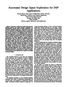
Fig. 8. A block scheme of the Hierarchical Fuzzy System used. SoC components (Proc, L1D$,L1I$ and L2D$) are modeled with a MIMO Fuzzy System, which is connected with others following the SoC hierarchy.
5.3
The Fuzzy System
The estimation block of the framework consists of a hierarchical FS [32] as shown in Figure 8. We split the system into three levels: the processor level, the L1 cache memory level, and the L2 cache memory level. A FS at level l uses as inputs the outputs of the FS at level l −1. For example, the FS used to estimate misses and hits in the first-level instruction cache uses as inputs the number of integer operations, float operations and branch operations estimated by the processor level FS as well as the cache configuration (size, block size, and associativity). This hierarchical decomposition of the system allows us to reduce drastically the complexity of the estimation problem with the additional effect of improving estimation accuracy. The knowledge base was defined on the basis of experience gained from an extensive series of tests. We verified that a fuzzy system with a few thousands rules takes milliseconds to approximate the objectives, which is some orders of magnitude less than the time required for a simulation. We therefore chose to use the maximum granularity, equal to the number of degrees of freedom for each input variable. The shape chosen for the sets was Gaussian intersecting at a degree of 0.5.
5.4
Assessment of Pareto set approximations
It is difficult to define appropriate quality measures for Pareto set approximations, and as a consequence graphical plots were until recently used to compare the outcomes of multi-objective algorithms. Nevertheless quality measures are necessary in order to compare the outcomes of multi-objective optimizers in a quantitative manner. Several quality measures have been proposed in the literature in recent years, an analysis and review of these is to be found in [33]. In this work we follow 18
the guidelines suggested in [34], that is a recent tutorial on performance assessment of stochastic multi-objective optimizers. The quality measures we considered most suitable for our context are the followings: (1) Hypervolume, This is a widely-used index, that measures the hypervolume of that portion of the objective space that is weakly dominated by the Pareto set to be evaluated. In order to measure this index the objective space must be bounded- if it is not, then a bounding reference point that is (at least weakly) dominated by all points should be used. In this work we define as bounding point the one which has coordinates in the objective space equal to the highest values obtained. Higher quality corresponds to smaller values. (2) Cardinality, this is an integer and represents the configurations selected for inclusion in the Pareto set. A high cardinality indicates that the designer has several solutions at his disposal, so can generally be considered to be positive. However, this index generally needs to be accompanied by others in order to provide significant information, because quantity is not always accompanied by quality. (3) Pareto Dominance, the value this index takes is equal to the ratio between the total number of points in Pareto set P that are also present in a reference Pareto set R (i.e. it is the number of non-dominated points by the other Pareto set). In this case a higher value obviously corresponds to a better Pareto set. Using the same reference Pareto set, it is possible to compare quantitatively results from different algorithms. (4) Distance, this index explains how close a Pareto set (P ) is to a reference set (R). We define the average and maximum distance index as follows: X
distanceaverage =
∀xi ∈P
min (d(xi , yj ))
∀yj ∈R
distancemax = max( min (d(xi , yj ))) xi ∈P ∀yj ∈R
where xi and yj are vectors whose size is equal to the number of objectives M and d(·, ·) is the Euclidean distance. The lower the value of this index, the more similar the two Pareto sets are. For example a high value of maximum distance suggests that some reference points are not well approximated, and consequently a high value of average distance tells us that an entire region of the reference Pareto is missing in the approximated set. A standard, linear normalization procedure was applied to allow the different objectives to contribute approximately equally to index values. In order to minimize differences in results due to the stochastic nature of GAs, we repeated the execution of the algorithm 10 times using different random seeds. For the analysis of multiple runs, we compute the quality measures of each individual run, and report the mean of these. 19
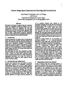
Fig. 9. Dependency graph of the parameterized VLIW-based system architecture.
6 Comparison between Methods
In this section we perform an extensive evaluation of the proposed approach by the comparison with the DSE approaches presented in Section 3. The comparison is carried out in terms of both accuracy and efficiency, on the parameterized system architecture described in Section 5. Efficiency can be defined as the number of system configurations simulated to complete the exploration, and is proportional to the execution time of the exploration algorithm. Accuracy is an index of quality of the solutions obtained. The parameters used for the GA-based approaches (GA and GA-Fuzzy) are as follows: The internal and external population were set as comprising 30 individuals, using a crossover probability of 0.8 and a mutation probability of 0.1. These values were set following the indications given in [21], where the convergence times and accuracy of the results were evaluated with various crossover and mutation probabilities, and it was observed that the performance of the algorithm with the various benchmarks was very similar. For GA-Fuzzy the estimation error is calculated in a window of 20 evaluations for the objectives, and the threshold was set to 5% of the Euclidean distance between the real point and estimated one in the objective space. The minimum number of evaluations, before which consider the error test to assess the reliability of the fuzzy estimator, was set to 90. Both thresholds were chosen after extensive series of experiments with computationally inexpensive test functions. The dependency graph used for DEP is depicted in Figure 9. It should be pointed out, however, that the dependency graph shown in Figure 9 is a simplified version of the actual dependency graph. This was due to the fact that it is unfeasible to apply DEP using the actual dependency graph, because exploration will run for a very long time. The logic followed was to remove some dependencies by requiring the parameters to be explored in order of importance. For example, we introduced an approximation whereby the parameters of the first level cache are explored independently of those of the second level cache. 20
Table 2 Parameters Space. Parameter
Parameter space
GPR / FPR
16,32,64,128
PR / CR
32,64,128
BTR
8,12,16
Integer/Float Units
1,2,3,4,5,6
Memory/Branch Units
1,2,3,4
L1D/I cache size
1KB,2KB,...,128KB
L1D/I cache block size
32B,64B,128B
L1D/I cache associativity
1,2,4
L2U cache size
32KB,64KB...,512KB
L2U cache block size
64B,128B,256B
L2U cache associativity
2,4,8,16
Space size
7.7397 × 10¹⁰
The parameter space along with the size of the design space to be explored is reported in Table 2. As can be seen, the size of the configuration space is such that to be able to explore all the configurations in a 365-day year a simulation need to last about 3 ms, a value which is several orders of magnitude away from the values in Table 1. A whole human lifetime would not, in fact, be long enough to obtain complete results for an exhaustive exploration of any of the existing benchmarks, even using the most powerful workstation currently available. It is, of course, possible to turn to High Performance Computing systems, but this is extremely expensive and would still require a very long time.
21
Table 3 GA-Fuzzy savings Benchmark
Number of
% Savings
simulations
of GA-Fuzzy vs.
GA-Fuzzy
GA
PBSA
DEP
GA
PBSA
DEP
wave
817
1412
3376
2378
42
76
66
fir
1563
2250
14941
17833
31
90
91
adpcm-encode
864
1373
5570
2096
37
84
59
adpcm-decode
962
1381
3257
1898
30
70
51
g721-encode
811
1354
6992
4654
40
88
83
jpeg-codec
1449
2254
12065
13642
36
88
89
mpeg2-dec
751
1389
4694
2892
46
84
74
38
83
73
Average % saving of GA-Fuzzy
For each benchmark Table 3 reports the number of configurations simulated by the different approaches. The table reports the percentage saving in number of simulations run by GA-Fuzzy respect to GA, PBSA, and DEP. On average, the exploration of the design space using GA-Fuzzy requires 38%, 73%, 83% less simulations than GA, PBSA, and DEP respectively. Considering the simulation time reported in Table 1 this translates in a saving in exploration time ranging from 3 hours for wave to 113 hours (i.e. about 5 days) for jpeg-codec. Learning and estimation times are neglected because they are several orders of magnitude shorter than simulation, as can be seen in Table 7.
22
Table 4 Quality assessment: distance from reference Pareto-optimal front. Benchmark
Distance from reference Pareto-optimal front% Average/Max (%) GA-Fuzzy
GA
PBSA
DEP
wave
0.18/0.97
0.24/6.65
1.24/8.41
0.59/7.52
fir
0.05/5.61
0.07/1.19
0.14/6.15
0.02/6.15
adpcm-encode
0.16/2.03
0.27/1.69
0.10/7.26
0.09/1.28
adpcm-decode
0.18/6.46
1.09/30.48
1.01/30.38
0.03/0.95
g721-encode
0.24/6.01
0.64/17.98
0.52/16.73
0.51/25.11
jpeg
0.83/7.76
0.62/6.90
0.12/1.93
0.80/4.07
mpeg2-decode
0.91/11.45
1.22/4.84
0.92/6.66
1.09/11.22
Average
0.36/5.76
0.59/9.96
0.58/11.07
0.45/8.04
To assess the accuracy of the different approaches, we need to know the Paretooptimal system configurations. Since the whole design space cannot be exhaustively explored in order to obtain them, we used the following approach to compute a reference Pareto-set. First, we merged all the Pareto-set obtained by each approach, then we removed all the dominated configurations. Thus, the remaining points, which are not dominated by any of the approximations sets, form the reference set. Table 4 reports the average and maximum distance between the Pareto fronts obtained by the different approaches and the reference Pareto front. As can be observed the accuracy exhibited by GA-Fuzzy is very close to that obtained by DEP. In particular for two of the benchmarks (wave and g721-encode) GAFuzzy outperforms the other approaches. As expected, DEP does not dominate the other approaches. In fact, as stated before, to make DEP computationally feasible, the dependency graph used in the experiments does not include all the parameters’ dependencies.
23
Table 5 Quality assessment: Hypervolume. Benchmark
Hypervolume (%) GA-Fuzzy
GA
PBSA
DEP
wave
25.19
25.44
28.41
26.69
fir
30.09
30.21
30.66
30.09
adpcm-encode
28.79
29.15
28.54
28.73
adpcm-decode
19.44
19.70
19.43
19.15
g721-encode
18.03
18.64
18.52
19.12
jpeg
16.31
16.61
15.90
16.33
mpeg2-decode
20.19
20.30
20.86
20.91
Average
22.58
22.86
23.18
23.00
To further confirm the accuracy of GA-Fuzzy, Table 5 reports the hypervolume measure (normalized respect to the boundaries of the objective space and expressed in percentage) of the Pareto-fronts obtained by the different approaches. Once again, the results confirm the accuracy characteristics of GA-Fuzzy. Actually, using this metric, all the approaches seem perform almost the same for all benchmarks. However, looking at the average results in Tables 4 and 5, it can be stated that GA-Fuzzy performs slightly better than the other approaches. Table 6 Accuracy comparison between GA and GA-Fuzzy after an equal number of simulations. Benchmark
Simulations
Cardinality
Pareto Dominance (%)
GA-Fuzzy
GA
GA-Fuzzy
GA
wave
1412
43
42
97.43
89.65
fir
2250
108
106
98.15
84.11
adpcm-encode
1373
53
48
82.55
68.22
adpcm-decode
1381
48
42
95.92
76.57
g721-encode
1354
118
118
74.81
59.85
jpeg
2254
166
127
74.95
64.87
mpeg2-dec
1389
157
152
80.22
54.72
Finally, in the last experiment, we perform the exploration of the design space by using GA and GA-Fuzzy on an equal number of simulations. Table 6 show that GAFuzzy yields a Pareto front which in many points dominates the set provided by GA thanks to its ability to evaluate much more system configurations than GA. This is 24
numerically expressed by the higher Pareto Dominance value and the greater number of points in the Pareto set obtained by the GA-Fuzzy approach. This means that the results obtained by GA-Fuzzy are both qualitatively and quantitatively better than that obtained by GA. In summary, the proposed approach yields similar results to those of the other approaches, with a 40–90% saving on computation time, which translates in several hours or days depending on the benchmark being considered. The equivalence of Pareto sets obtained is numerically justified by the short distance between the sets and the similar hypervolume values. Table 7 Efficiency and accuracy of fuzzy estimation system builded by GA-Fuzzy on a random test set of 10,000 configurations Benchmark fir
adpcm-enc
adpcm-dec
mpeg2-dec
jpeg
g721-enc
Simulations
2250
1373
1381
1389
2254
1354
Rules
2172
1338
1342
1354
2168
1313
- Learn
3.44
3.36
3.39
3.81
5.37
3.09
- Estimate
6.87
6.72
6.88
7.51
10.68
6.26
Avg Time (ms)
Avg Estimation Error (%) Whole Set - Avg Power
6.76
8.12
7.13
12.12
7.08
7.41
- Exec Time
6.33
8.01
7.02
18.89
6.07
6.42
- Avg Power
2.21
2.41
2.22
7.88
2.88
2.72
- Exec Time
4.21
3.45
4.99
8.21
2.49
4.04
Pareto Set
Another interesting feature of the approach proposed is that at the end of the genetic evolution we obtain a fuzzy system that can approximate any configuration. The designer can exploit this to conduct a more in-depth exploration. Table 7 gives the estimation errors for the fuzzy system obtained after 100 generations on a random set of configurations other than those used in the learning phase. The same table also shows the time required to simulate a system configuration on a Pentium IV 2.8GHz workstation. Despite the great number of rules this time is several orders of magnitude shorter as compared to the time required to perform a simulation without any appreciable impact on estimation accuracy.
25
PBSA DEP GA GAF
0.125
Execution Time (ms)
0.12
0.115
0.11
0.105
0.1
0.095
0.09 1.5
1.6
1.7
1.8
1.9
2
Average Power Consumption (W)
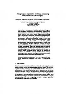
Fig. 10. wave: Pareto sets and attainment surfaces obtained by DEP, PBSA, GA and GA– Fuzzy (GAF). 62
PBSA DEP GA GAF
60
58
Execution Time (ms)
56
54
52
50
48
46
44
42 1.4
1.45
1.5
1.55
1.6
1.65
1.7
1.75
Average Power Consumption (W)
Fig. 11. adpcm-encoder: Pareto sets and attainment surfaces obtained by DEP, PBSA, GA and GA-Fuzzy (GAF).
7 Conclusion and Future Works
In this paper we presented a new DSE approach based on a Hierarchical Fuzzy System hybridized with a Genetic Algorithm. The approach reduces the number of 26
simulations while minimizing the time required to simulate: GA smartly explores the design space, in the meanwhile the FS learn from the experience accumulated during the GA evolution, storing knowledge in fuzzy rules. The joined rules build the Knowledge Base through which the integrated system quickly predict the results of complex simulations thus avoiding their long execution times. A comparison between GA-Fuzzy and established DSE approaches, performed on various multimedia benchmarks, showed that integration with the fuzzy system saves a great amount of time and also gives slightly more accurate results. Further developments may involve the use of acquired knowledge to create a set of generic linguistic rules to speed up the learning phase, providing an aid for designers and a basis for teaching. Finally, we are interested in applying the estimation technique by means of a fuzzy system to the other approaches as well, with a view to speeding them up.
References
[1] F. Vahid, T. Givargis, Platform tuning for embedded systems design, IEEE Computer 34 (3) (2001) 112–114. [2] T. Givargis, F. Vahid, J. Henkel, System-level exploration for Pareto-optimal configurations in parameterized System-on-a-Chip, IEEE Transactions on Very Large Scale Integration Systems 10 (2) (2002) 416–422. [3] W. Fornaciari, D. Sciuto, C. Silvano, V. Zaccaria, A sensitivity-based design space exploration methodology for embedded systems, Design Automation for Embedded Systems 7 (2002) 7–33. [4] G. Ascia, V. Catania, M. Palesi, A multi-objective genetic approach for system-level exploration in parameterized systems-on-a-chip, IEEE Transactions on ComputerAided Design of Integrated Circuits and Systems 24 (4) (2005) 635–645. [5] G. Hekstra, D. L. Hei, P. Bingley, F. Sijstermans, TriMedia CPU64 design space exploration, in: International Conference on Computer Design, Austin Texas, 1999, pp. 599–606. [6] S. G. Abraham, B. R. Rau, R. Schreiber, Fast design space exploration through validity and quality filtering of subsystem designs, Tech. Rep. HPL-2000-98, HP Laboratories Palo Alto (Jul. 2000). [7] R. Szymanek, F. Catthoor, K. Kuchcinski, Time-energy design space exploration for multi-layer memory architectures, in: Design, Automation and Test in Europe, 2004, pp. 181–190. [8] S. Neema, J. Sztipanovits, G. Karsai, Design-space construction and exploration in platform-based design, Tech. Rep. ISIS-02-301, Institute for Software Integrated Systems Vanderbilt University Nashville Tennessee 37235 (Jun. 2002). [9] A. Ghosh, T. Givargis, Cache optimization for embedded processor cores: An analytical approach, ACM Transactions on Design Automation of Electronic Systems, 9 (4) (2004) 419–440.
27
[10] L. Eeckhout, S. Nussbaum, J. E. Smith, K. D. Bosschere, Statistical simulation: Adding efficiency to the computer designer’s toolbox, IEEE Micro 23 (5) (2003) 26– 38. [11] S. Eyerman, L. Eechhout, K. D. Bosschere, Efficient design space exploration of high performance embedded out-of-order processors, in: DATE, 2006. [12] P. Mazumder, E. M. Rudnick, Genetic Algorithms for VLSI Design, Layout & Test Automation, Prentice Hall, Inc., 1999. [13] C. J. Alpert, L. W. Hagen, A. B. Kahng, A hybrid multilevel/genetic approach for circuit partitioning, in: Fifth ACM/SIGDA Physical Design Workshop, 1996, pp. 100– 105. [14] K. Shahookar, P. Mazumder, A genetic approach to standard cell placement using metagenetic parameter optimization, IEEE Transactions on Computer-Aided Design 9 (1990) 500–511. [15] J. Lienig, K. Thulasiraman, A genetic algorithm for channel routing in VLSI circuits, Evolutionary Computation 1 (4) (1993) 293–311. [16] Y.-M. Jiang, K.-T. Cheng, A. Krstic, Estimation of maximum power and instantaneous current using a genetic algorithm, in: Proceedings of IEEE Custom Integrated Circuits Conference, 1997, pp. 135–138. [17] V. Kommu, I. Pomenraz, GAFAP: Genetic algorithm for FPGA technology mapping, in: European Design Automation Conference, 1993, pp. 300–305. [18] C. J. Alpert, A. B. Kahng, Recent developments in netlist partitioning: A survey, VLSI Journal 19 (1–2) (1995) 1–81. [19] D. Saab, Y. Saab, J. Abraham, Automatic test vector cultivation for sequential VLSI circuits using genetic algorithms, IEEE Transactions on Computer-Aided Design 15 (10) (1996) 1278–1285. [20] G. Ascia, V. Catania, M. Palesi, Parameterized system design based on genetic algorithms, in: 9th. International Symposium on Hardware/Software Co-Design, Copenhagen, Denmark, 2001, pp. 177–182. [21] G. Ascia, V. Catania, M. Palesi, A GA based design space exploration framework for parameterized system-on-a-chip platforms, IEEE Transactions on Evolutionary Computation 8 (4) (2004) 329–346. [22] W. Fornaciari, D. Sciuto, C. Silvano, V. Zaccaria, A design framework to efficiently explore energy-delay tradeoffs, in: 9th. International Symposium on Hardware/Software Co-Design, Copenhagen, Denmark, 2001, pp. 260–265. [23] G. Ascia, V. Catania, M. Palesi, Tuning methodologies for parameterized systems design, in: K. A. Publisher (Ed.), System on Chip for Realtime Systems, 2002. [24] E. Zitzler, M. Laumanns, L. Thiele, SPEA2: Improving the performance of the strength pareto evolutionary algorithm, in: EUROGEN 2001. Evolutionary Methods for Design, Optimization and Control with Applications to Industrial Problems, Athens, Greece, 2001, pp. 95–100.
28
[25] E. Zitzler, L. Thiele, Multiobjective evolutionary algorithms: A comparative case study and the strength pareto approach, IEEE Transactions on Evolutionary Computation 4 (3) (1999) 257–271. [26] L.-X. Wang, J. M. Mendel, Generating fuzzy rules by learning from examples, IEEE Transactions on System, Man and Cybernetics 22 (1992) 1414–1427. [27] T. Takagi, M. Sugeno, Fuzzy identification of systems and its application to modeling and control, IEEE Transactions on System, Man and Cybernetics 15 (1985) 116–132. [28] J. A. Fisher, Very long instruction word architectures and the ELI512, in: Tenth Annual International Symposium on Computer Architecture, 1983, pp. 140–150. [29] An infrastructure for research in instruction-level parallelism, http://www. trimaran.org/. [30] G. Ascia, V. Catania, M. Palesi, D. Patti, EPIC-Explorer: A parameterized VLIWbased platform framework for design space exploration, in: First Workshop on Embedded Systems for Real-Time Multimedia (ESTIMedia), Newport Beach, California, USA, 2003, pp. 65–72. [31] D. Patti, M. Palesi, EPIC-Explorer, http://epic-explorer.sourceforge. net/ (Jul. 2003). [32] X.-J. Zeng, J. A. Keane, Approximation capabilities of hierarchical fuzzy systems, IEEE Transactions on Fuzzy Systems 13 (5) (2005) 659–672. [33] E. Zitzler, L. Thiele, M. Laumanns, C. M. Fonseca, V. G. da Fonseca, Performance assessment of multiobjective optimizers: An analysis and review, IEEE Transactions on Evolutionary Computation 7 (2) (2003) 117–132. [34] J. D. Knowles, L. Thiele, E. Zitzler, A tutorial on the performance assessment of stochastive multiobjective optimizers, Tech. Rep. TIK-Report No. 214, Computer Engineering and Networks Laboratory, ETH Zurich, Swiss (Feb. 2006). URL http://dbk.ch.umist.ac.uk/knowles/TIK214b.pdf
29