Multi-Objective Differential Evolution (MODE): An Evolutionary Algorithm for Multi-Objective Optimization Problems (MOOPs) B. V. Babu* and B. Anbarasu Birla Institute of Technology and Science (BITS) PILANI – 333 031 (Rajasthan) INDIA
[email protected] Abstract
The last decade has seen a surge of research activity on Multi-objective Optimization using evolutionary computation and a number of algorithms have been developed. Although Evolutionary Algorithms (EAs) are successful, to some extent, in solving Multi-Objective Optimization Problems (MOOPs), the methods appearing in the literature vary a lot in terms of their solutions and the way of comparing their best results with other existing algorithms. In other words, there is no well-accepted method for MOOPs that will produce a good set of solutions for all problems. This motivates the further development of good approaches to MOOPs. In this paper, we propose a novel approach using Differential Evolution (DE) for MOOPs, referred to herein as Multi-Objective Differential Evolution (MODE). The performance of MODE has been compared to that of other Elitist multi-objective evolutionary algorithms such as NSGA-II and its adapted form, NSGA-II-JG on four test problems. It has been observed that even though the computational complexity of MODE is high, the solutions obtained on the pareto optimal front are well diversed. Index Terms — Evolutionary Computation, Differential Evolution, Evolutionary Multi-objective Optimization (EMO), Multi-Objective Differential Evolution (MODE).
1. Introduction Till the last decade, most of the problems solved in the field of optimization involved only a single objective function. In the past several years, there has been an increasing interest in applying evolutionary algorithms to multiobjective optimization problems (MOOPs), since real world optimization problems often involve several conflicting objectives. *Corresponding Author:
Assistant Dean-ESD & Head-Chemical Engineering Department BITS, PILANI-333 031 (Rajasthan) India Phone: 0091-1596-245073 Ext. 205/224; Fax: 0091-1596-244183; E-mail:
[email protected] Homepage: http://discovery.bits-pilani.ac.in/discipline/chemical/BVb/
In such multiobjective studies, we often obtain a Pareto set of non-dominating (equally good) solutions, and a decisionmaker needs to use his intuition or additional information to decide upon the preferred solution. Indeed, Deb [1] has given several examples in different fields that are better studied using multiple objectives.
2. Elitist Multi-Objective Algorithms
Evolutionary
During the past few years, a number of different Evolutionary Algorithms (EAs) were suggested to solve multi-objective optimization problems. An elitist nondominated sorting genetic algorithm (NSGA-II) was proposed by Deb et al. [2]. NSGA-II has several advantages over the currently available multi-objective optimization algorithms. These have been reviewed by Deb [1]. NSGA-II uses the concept of elitism, borrowed from nature. Two main features of the algorithm are as follows: i) assigning fitness to population members based on nondominated sorting and ii) preserving diversity among solutions of the same nondominated front. In this algorithm, the better parents are given a chance to be part of the next generation. In contrast, the likelihood of this happening in the earlier algorithm, NSGA-I, that did not incorporate this concept, is very small. Unfortunately, the diversity decreases because of this elitism, and this needs to be counteracted by some means. One such adaptation, inspired by the concept of jumping genes (JG, or transposons) in biology, was developed by Kasat and Gupta [3]. This is referred to as NSGA-II-JG. This adaptation exploits the benefits of elitism, while still maintaining genetic diversity. In this study, Differential Evolution (a highly efficient optimization algorithm for single objective problems), has been adapted for solving optimization problems involving multiple objectives. It has been applied to four different test problems chosen from Deb [1] and the results have been compared to that obtained using NSGA-II and NSGA-II-JG. The results encourage
the application of MODE to more complex and realworld multi-objective optimization problems.
3. Differential Evolution
( )
' xi ,G = k = lower xi +
Differential Evolution (DE) is a type of evolutionary algorithm originally proposed by Price and Storn [4] for optimization problems over a continuous domain. DE is similar to a (µ, ) evolution strategy in which mutation plays the key role. The basic idea of DE is to adapt the search during the evolutionary process. At the start of evolution, the perturbations are large since parent individuals are far away from each other. As the evolutionary process matures, the population converges to a small region and the perturbations adaptively become small. As a result, the evolutionary algorithm performs a global exploratory search during the early stages of the evolutionary process and local exploitation during the mature stage of the search. In DE, a solution, l, in a generation is a multidimensional vector x G =i = ( x1 ,......., x N )T . A population, l
PG =k , at generation G=k is a vector of M solutions
{
1
M
}
(M>4). The initial population, PG =0 = x G =0 ,......, x G =0 , is initialized as
( )
[ ] (
( )
( )),
l x i,G =0 = lower x i + rand i 0,1 × upper x i − lower x i l = 1,......, M
l
the initial generation G = 0, x i ,G = 0 , is initialized within its boundaries (lower(xi ), upper(xi )) . Selection is carried out to select four different solutions indices r1; r2; r3; and j ∈ [1,M]. The values of each variable in the child are changed with some crossover probability, CR, to
(
r r r x i ,3G = k −1 + F × x i 1,G = k −1 − x i ,2G =k −1 if
(random[0,1] < CR ∧ i = i rand )
if
2 j xi ,G − upper xi
( )
( )
j xi ,G +1 < lower xi if
2 j xi ,G +1 otherwise
( )
j xi ,G +1 > upper xi
The detailed algorithm is available in literature [8,9].
4. Different Strategies of DE Price & Storn [4] gave the working principle of DE with single strategy. Later on, they suggested ten different strategies of DE. The strategies can vary based on the vector to be perturbed, number of difference vectors considered for perturbation, and finally the type of crossover used [4,8]. However, strategy-7 (DE/rand/1/bin) is the most successful and the most widely used strategy. The key parameters of control in DE are: NP-the population size, CR-the crossover constant, and F-the weight applied to random differential (scaling factor). In addition, some new strategies have been proposed and successfully applied to optimization of extraction process by Babu & Angira [6]. DE has been successfully applied in various fields [7-22].
5. Multi-Objective Differential Evolution
i = 1, 2,......, N
where, M is the population size, N is the solution’s dimension, and each variable i in a solution vector l in
' ∀i ≤ N , x i ,G =k =
( )
j xi ,G + lower xi
)
j x i ,G =k −1 otherwise
where, F ∈ (0, 1) is a problem parameter representing the amount of perturbation added to the main parent. The new solution replaces the old one if it is better than the original and at least one of the variables should be changed. The latter is represented in the algorithm by randomly selecting a variable, irand (1, N). After crossover, if one or more of the variables in the new solution are outside their boundaries, the following repair rule is applied.
This is inspired from elitist nondominated sorting genetic algorithm (NSGA-II). In a single-objective optimization problem, the best solution, integral to the DE search process, may be easily identified by selecting the individual with highest fitness value. However, in a multi-objective domain, the goal is to identify the Pareto optimal solution set. In this proposed multi-objective differential evolution (MODE), a Pareto-based approach is introduced to implement the selection of the best individuals. Firstly, a population of size, NP, is generated randomly and the fitness functions are evaluated. At a given generation of the evolutionary search, the population is sorted into several ranks based on dominance concept. Secondly, DE operations are carried out over the individuals of the population. The fitness functions of the trial vectors, thus formed, are evaluated. One of the major differences between DE and MODE is that the trial vectors are not compared with the corresponding parent vectors. Instead, both the parent vectors and the trial vectors are combined to form a global population of size, 2*NP. Then, the ranking of the global population is carried out followed by the crowding distance calculation. The best NP individuals are selected based on its ranking and crowding distance. These act as the parent vectors for the next generation.
The procedure is carried out until the entire selected best NP individuals have a rank of one. The Pseudocode for MODE algorithm is presented below: The following assumes that we are minimizing all the objective functions, fq (1) Generate box, P, of Np parent vectors using a random-number code to generate the several real variables. These vectors are given a sequence (position) number as generated (2) Classify these vectors into fronts based on nondomination [1], as follows: a. Create new (empty) box, P’, of size, Np b. Transfer ith vector from P to P’, starting with i=1 c. Compare vector I with each member, say each member, say j, already present in P’, one at a time d. If i dominates31 over j (i.e. i is superior to or better than j in terms of all objective functions), remove the jth vector from P’ and put it back in its original location in P e. If i dominated over by j, remove i from P’ and put it back in its position in P f. If i and j are non-dominating (i.e. there is at least one objective function associated with i that is superior to/better than that of j), keep both i and j in P’ (in sequence). Test for all j present in P’ g. Repeat for next vector (in the sequence, without going back) in P till all Np are tested. P’ now contains a sub-box (of size CR; copy the value from the target vector, else copy the value from the noisy random vector into the trial vector and put it in box P’’ (5) Elitism: Copy all the Np parent vectors (P’) and all the Np trial vectors (P’’) into box PT. Box PT has 2Np vectors a. Reclassify these 2Np vectors into fronts (box PT’) using only non-domination (as described in Step 2 above) b. Take the best Np from box PT’ and put into box P’’’. The following procedure is adopted to identify the better of the two chromosomes. Chromosome i is better than chromosome j if Ii,rank ≠ Ij,rank : Ii,rank < Ij,rank Ii,rank =Ij,rank : Ii,dist > Ij,dist This completes one generation. Stop if appropriate criteria are met, e.g., the generation number > maximum number of generations (user specified). Else, Copy P’’’ into starting box, P. Go to Step 2 above
6. Test Problems The test problems were taken from Deb [1]. We first describe the test problems used to compare different algorithms. Problem 1: Min. f1(x) = x1; 0.1 x1 1 Min. f2(x) = (1+x2)/x1; 0 x2 5 Problem 2:
7.2 Results
Max. f1(x) =1-x1; 0.1 x1 1 Max. f2 = 60-(1+x2)/x1; 0 x2 5 Problem 3: πd 2 Min f1 (d , l ) = ρ l 10 ≤ d ≤ 50mm 4 64 PI 3 Min f 2 (d , l ) = 200 ≤ l ≤ 1000mm 3Eπd 4 subject to
The results obtained for various cases are presented in the form of tables (Tables 2-5). Table 2 Effects of NP and other parameters on different Algorithms for Case-I Algorithm Parameter
σ max ≤ S , δ ≤ δ max
NSGA-II
where, the maximum stress is calculated as follows : 32 PI σ max = πd 3
The following parameter values are used: =7800 kg/cu. m P = 1000 N E = 207 GPa Sy=300 MPa max = 5 mm Problem 4:
(
)
(
Min
f1 (x ) = 0.5 x12 + x22 + sin x12 + x22
Min
f 2 (x ) =
(3 x1 − 2 x 2 + 4 )2 + (x1 − x 2 + 1)2
f 3 (x ) =
Min
)
8
(x
2 1
1
27
− 1.1e (− x1 − x 2 ) 2
)
+ x +1 2 2
2
+ 15
NSGA-IIJG (Pjump)
MODE (Scaling Factor-F)
2
Table-1 shows the details of the Case-I to Case-VIII. Single point Cross-over is used. Mutation Probability for NSGA-II & NSGA-II-JG - 0.05 Table-1 Details of Cases I to VIII 1
Case II
2
Case III
3
Case IV
1
Case V
3
Case VI
3
Case VII
3
Case VIII
4
Scaling Factor, F
0.5 11 11 10 11 11 11 12 12 11 11
7.1 Case Studies
Case I
Scaling Factor, F
0.5 0.6 0.7 0.8 0.9 0.5 0.6 0.7 0.8 0.9
Several cases have been studied using the test problems. This section deals with the results obtained for various cases and the related inferences.
Type/ DE strategy Unconstrained DE/rand/1/bin Unconstrained DE/rand/1/bin Constrained DE/rand/1/bin Unconstrained DE/rand/1/bin Constrained DE/rand/1/bin Constrained DE/rand/1/exp Constrained DE/current-torand/1/bin Unconstrained DE/rand/1/bin
Pop = 100 Time, Gen ms 7 563 7 578 8 672 9 734 9 734 9 750 11 875 12 953 11 875 14 1110 15 1187
Generation for Case IV Generation for Case V Parameter
7. Results and Discussion
Problem No.
Pop = 40 Time, Gen ms 7 500 10 718 8 578 7 500 9 641 8 562 11 781 9 641 9 641 10 703 11 766
Table 3 Effects of CR and F on Generations in MODE for Case IV & Case V
- 3 ≤ x1 , x 2 ≤ 3
Case
0.5 0.6 0.7 0.8 0.9 0.5 0.6 0.7 0.8 0.9
Pop = 20 Time, Gen ms 10 672 7 468 7 469 8 546 9 625 8 547 8 516 6 406 6 406 11 750 6 406
Accuracy CR Np
Random Seed
x1-0.001 0.95 0.7534 x2-0.001 x1-0.001 0.95 - 0.6985414 x2-0.001 d-0.0001 0.95 0.28446 l-0.001 d-0.0001 - 100 0.7534 l-0.001 d-0.0001 - 100 0.28446 l-0.001 d-0.0001 - 100 0.28446 l-0.001 d-0.0001 l-0.001
-
100
0.28446
x1-0.001 x2-0.001
-
100
0.35652
0.6 10 11 10 11 11 11 10 12 13 13 CR 0.7 11 13 11 11 12 12 13 13 12 14 0.8 11 11 12 12 13 12 13 14 13 13 0.9 11 12 14 13 13 13 12 13 14 15
Table 4 Effects of NP and other parameters on different algorithms for Case II Algorithm Parameter NSGA-II NSGA-IIJG (Pjump)
MODE (Scaling Factor-F)
0.5 0.6 0.7 0.8 0.9 0.5 0.6 0.7 0.8 0.9
Pop = 20 Gen 5 5 6 5 6 6 9 8 7 9 6
Time, ms 328 344 422 344 406 407 625 547 469 609 406
Pop = 40 Gen 8 8 6 7 8 7 11 10 11 11 10
Time, ms 563 563 422 500 578 500 734 703 766 766 703
Pop = 100 Gen 8 8 10 10 9 9 11 11 11 14 13
Time, ms 688 656 828 813 734 734 859 859 860 1109 1031
Table 5 Effects of NP and Other parameters on different Algorithms for CASE III
NSGA-II NSGA-IIJG (Pjump)
MODE (Scaling Factor-F)
-
7
Time, ms 485
0.5 0.6 0.7 0.8 0.9 0.5 0.6 0.7 0.8 0.9
5 9 7 7 6 7 8 7 7 9
328 625 485 485 422 469 546 469 468 609
Gen
Pop = 40
6
Time, ms 437
8 8 8 7 10 11 10 11 13 10
578 578 563 516 719 782 703 782 938 703
Gen
8
Time, ms 687
8 10 9 10 10 13 14 13 15 16
687 844 767 859 859 1078 1156 1078 1234 1312
Gen
NSGA -II
Pop - 100
10
Pop = 100
NSGA -II-JG(0.9) M ODE(0.5)
8 6
f2
Algorithm Parameter
Pop = 20
12
4 2 0 0
0.2
0.4
0.6
0.8
1
f1
Fig. 1(b). Effects of NP and other parameters on different algorithms for Case I
7.3 Discussion
18
M ODE(0.5)
12 10 8 6 4 2 0 0
0.2
0.6
0.8
1
Fig. 1(c). Effects of NP and other parameters on different algorithms for Case I Effect of Number of Generations: Once the entire population reaches the first front, a slight increase in the number of generation increases the diversity of the solution. However, for a very high value of generation the diversity decreases and the computational time increases. 60
NSGA -II
NSGA -II
Pop - 20
NSGA -II-JG(0.6)
10
0.4 f1
12 Pop - 40
NSGA -II-JG(0.7)
14
f2
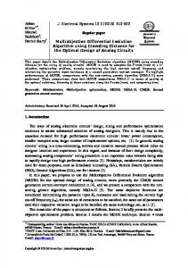
The inferences obtained from the results are discussed in terms of the following: population size, number of generation, controlling parameters and different strategies. Effect of Population Size: It can be observed from Figs. 1-3 that NSGA-II could converge to the global optimum even with a population size of 20 as compared to NSGA-II-JG and MODE. However, the solutions obtained using NSGA-II are less diverse. For all the three algorithms, computational complexity increases with the population size. For a population size of 100, all the three algorithms converged to the Pareto set. Hence in most of the Multiobjective Optimization Problems (MOPs), the population size is taken as 100. The number of generations required for convergence is presented in Table 2, Table-4 and Table-5.
NSGA -II
Pop - 20
16
NSGA -II-JG(0.8)
58
M ODE(0.8)
M ODE(0.5)
8
f2
f2
56 6 4
54 52
2
50
0 0
0.2
0.4
0.6
0.8
1
f1
48 0
Fig. 1(a). Effects of NP and other parameters on different algorithms for Case I
0.2
0.4
0.6
0.8
1
f1
Fig. 2(a). Effects of NP and other parameters on different algorithms for CaseII
0.005
60
NSGA -II-JG(0.9)
58
NSGA -II
Pop - 20
NSGA -II
Pop - 40
NSGA -II-JG(0.6) M ODE(0.7)
0.004
M ODE(0.9)
56 f2
f2
0.003
54
0.002
52 0.001
50 0 0.6
48 0
0.2
0.4
0.6
0.8
f1
Fig. 2(b). Effects of NP and other parameters on different algorithms for CaseII 60
1.1
2.6
3.1
Fig. 3(b). Effects of NP and other parameters on different algorithms for Case III 0.005
NSGA -II-JG(0.7)
58
2.1 f1
NSGA -II
Pop - 100
NSGA -II
Pop - 100
1.6
1
NSGA -II-JG(0.8) M ODE(0.9)
0.004
M ODE(0.5)
56 f2
f2
0.003
54
0.002
52
0.001
50 0 0.6
48 0
0.2
0.4
0.6
0.8
1
f1
Fig. 2(c). Effects of NP and other parameters on different algorithms for CaseII Effect of Key Parameters: For a population size of 100, NSGA-II-JG is found to perform well (in terms of both Pareto set and diversity) with PJUMP=0.7 and Pcross= 0.95, in most of the cases. This is well evident from Table 2, Table-4 and Table-5. It is also suggested not to choose high value of PJUMP, as it increases the number of generation. As far as MODE is concerned, it is observed from Table 3 and Table-5 that the following combinations of CR and F provide excellent result for the two objective problems. 0.005
NSGA -II
Pop - 40
NSGA -II-JG(0.5) M ODE(0.5)
0.004
f2
0.003
0.002
0.001
0 0.6
1.1
1.6
2.1
2.6
3.1
f1
Fig. 3(a). Effects of NP and other parameters on different algorithms for Case III
1.1
1.6
f1
2.1
2.6
3.1
Fig. 3(c). Effects of NP and other parameters on different algorithms for Case III Crossover Probability (CR) Scaling Factor (F) Low Low Low High High Low For any number of objective functions, it is better to choose the following range of values for F and CR: 0.5 – 0.7 and 0.7 – 0.9 respectively. Effect of Different Strategies on MODE: The following strategies of DE have been studied for their performance: I. DE/rand/1/bin II. DE/rand/1/exp III. DE/current-to-rand/1/bin It is found that the first strategy performs better in terms of both Pareto set and diversity. In normal DE, the trial vector replaces the parent vector in the next generation if it has better fitness value. It is not so in MODE as the child vectors are chosen from the global competition. Thus, the randomness of the DE is greatly affected and would have lead to the premature convergence of the algorithm at a low population. However, for a large population size, the algorithm could converge to global pareto set. This increases the run-time complexity of the algorithm.
8. Conclusions The major advantage of the MODE over other existing algorithms is its diversity. Thus it is concluded that MODE could be applied to the more complicated systems where other algorithms fail to provide diverse solutions. It also provides an alternative means to solve MOPs. Yet, the run-time complexity of MODE is an area that has to be explored for further improvement. [1] [2]
[3]
[4] [5]
[6]
[7]
[8] [9] [10]
[11]
[12]
[13]
[14]
References
K. Deb, Multi-objective Optimization using Evolutionary Algorithms. Chichester, U.K.: Wiley, 2001. K. Deb, S. Agarwal, A. Pratap and T. Meyariyan, “A Fast and Elitist Multiobjective Genetic Algorithm: NSGA-II,” IEEE Transactions on Evolutionary Computation, vol. 6, no. 2, pp. 182197, April 2002. Rahul B. Kasat and Santosh K. Gupta, “Multi-objective optimization of an industrial fluidized-bed catalytic cracking unit (FCCU) using genetic algorithm (GA) with the jumping genes operator, ” Computers & Chemical Engineering, vol. 27, no. 12, pp. 1785-1800, December 2003. K. Price and R. Storn, “Differential Evolution – A simple evolution strategy for fast optimization,” Dr.Dobb’s Journal, vol. 22, no. 4, pp. 18-24, April 1997. H. A. Abbass and R. Sarker, “The Pareto Differential Evolution Algorithm, ” International Journal on Artificial Intelligence Tools, Vol. 11, No. 4, pp. 531-552, December 2002.
B. V. Babu and Rakesh Angira, “New Strategies of Differential Evolution for Optimization of Extraction Process,” presented at the 2003 International Symposium & 56th Annual Session of IIChE (CHEMCON), Bhubaneswar. B. V. Babu and K. K. N. Sastry, “Estimation of Heat Transfer Parameters in a Trickle Bed Reactor using Differential Evolution and Orthogonal Collocation”, Computers and Chemical Engineering, Vol. 23 (No. 3), pp. 327-339, 1999. B. V. Babu, Process Plant Simulation. New Delhi, India: Oxford University Press, 2004. G. C. Onwubolu and B. V. Babu, New Optimization Techniques in Engineering. Heidelberg, Germany: Springer-Verlag, 2004. B. V. Babu and S.A.Munawar, “Differential Evolution for the Optimal Design of Heat Exchangers”, Proceedings of All India Seminar on “Chemical Engineering Progress on Resource Development: A Vision 2010 and Beyond”, organized by IE (I), Orissa State Centre Bhuvaneshwar, March 13, 2000. B. V. Babu and Rishindra Pal Singh, “Optimization and Synthesis of Heat Integrated Distillation Systems Using Differential Evolution”, Proceedings of All India Seminar on “Chemical Engineering Progress on Resource Development: A Vision 2010 and Beyond”, organized by IE (I), Orissa State Centre Bhuvaneshwar, March 13, 2000. B. V. Babu and Gaurav Chaturvedi, “Evolutionary Computation strategy for optimization of an Alkylation Reaction”, Proceedings of International Symposium & 53rd Annual Session of IIChE (CHEMCON-2000), Science City, Calcutta, December 18-21, 2000. B. V. Babu and Rakesh Angira, “Optimization of Non-Linear Functions Using Evolutionary Computation”, Proceedings of 12th ISME Conference on Mechanical Engineering, Crescent Engineering College, Chennai, January 10-12, 2001, Paper No. CT07, pp. 153-157 (2001). B. V. Babu and S.A.Munawar, “Optimal Design of Shell-andTube Heat Exchangers using Different Strategies of Differential Evolution”, PreJournal.org – The Faculty Lounge, Article No. 003873, posted on website Journal http://www.prejournal.org, March 03, 2001.
[15] B. V. Babu and Rakesh Angira, “Optimization of Thermal Cracker Operation using Differential Evolution”, Proceedings of International Symposium & 54th Annual Session of IIChE (CHEMCON-2001), CLRI, Chennai, December 19-22, 2001. [16] B. V. Babu and K.Gautam, “Evolutionary Computation for Scenario-Integrated Optimization of Dynamic Systems”, Proceedings of International Symposium & 54th Annual Session of IIChE (CHEMCON-2001), CLRI, Chennai, December 19-22, 2001. [17] B. V. Babu and Rakesh Angira, “A Differential Evolution Approach for Global Optimization of MINLP Problems”, Proceedings of 4th Asia-Pacific Conference on Simulated Evolution And Learning (SEAL' 02), Singapore, November 18 22, 2002, Paper No. 1033, Vol. 2, pp. 880-884, 2002 [18] B. V. Babu and Rakesh Angira, “Optimization of Non-Linear Chemical Processes Using Evolutionary Algorithm”, Proceedings of International Symposium & 55th Annual Session of IIChE (CHEMCON-2002), OU, Hyderabad, December 19-22, 2002. [19] Rakesh Angira and B. V. Babu, “Evolutionary Computation for Global Optimization of Non-Linear Chemical Engineering Processes”, Proceedings of International Symposium on Process Systems Engineering and Control (ISPSEC’03) - For Productivity Enhancement through Design and Optimization, IIT-Bombay, Mumbai, January 3-4, 2003, Paper No. FMA2, pp. 87-91 (2003). [20] B. V. Babu and Rakesh Angira, ”Optimization of Water Pumping System Using Differential Evolution Strategies”, Proceedings of The Second International Conference on Computational Intelligence, Robotics, and Autonomous Systems (CIRAS-2003), Singapore, December 15-18, 2003. [21] B. V. Babu, Rakesh Angira, Pallavi G.Chakole, and J.H.Syed Mubeen, “Optimal Design of Gas Transmission Network using Differential Evolution”, Proceedings of The Second International Conference on Computational Intelligence, Robotics, and Autonomous Systems (CIRAS-2003), Singapore, December 1518, 2003. [22] B. V. Babu, Rakesh Angira, and Anand Nilekar, “Optimal Design of an Auto-Thermal Ammonia Synthesis Reactor Using Differential Evolution”, Proceedings of The Eighth World MultiConference on Systemics, Cybernetics and Informatics (SCI2004), July 18-21, 2004, Orlando, Florida, USA. Note: The soft copies of full papers in PDF format of the references in which B.V. Babu is one of the authors as listed above are available at the homepage of B.V.Babu, the URL of which is http://discovery.bitspilani.ac.in/discipline/chemical/BVb/publications/html.