Feb 4, 2004 - that the multi-objective optimization genetic algorithm returns a set of .... route-second method using genetic algorithms and local search optimization ...... The Theory of NP-Completeness, W. H. Freeman and Company, 1979.
Brock University Department of Computer Science
Multi-objective Genetic Algorithms for Vehicle Routing Problem with Time Windows B. Ombuki, B. J. Ross, and F. Hanshar Technical Report # CS-04-02 January 2004
Brock University Department of Computer Science St. Catharines, Ontario Canada L2S 3A1 www.cosc.brocku.ca
Multi-Objective Genetic Algorithms for Vehicle Routing Problem with Time Windows Beatrice Ombuki, Brian J. Ross and Franklin Hanshar Brock University. Dept. of Computer Science St. Catharines, ON, Canada L2S 3A1 {bross, bombuki}@cosc.brocku.ca February 4, 2004 ABSTRACT The Vehicle Routing Problem with Time windows (VRPTW) is an extension of the capacity constrained Vehicle Routing Problem (VRP). The VRPTW is NP-Complete and instances with 100 customers or more are very hard to solve optimally. We represent the VRPTW as a multi-objective problem and present a genetic algorithm solution using the Pareto ranking technique. We use a direct interpretation of the VRPTW as a multi-objective problem, in which the two objective dimensions are number of vehicles and total cost (distance). An advantage of this approach is that it is unnecessary to derive weights for a weighted sum scoring formula. This prevents the introduction of solution bias towards either of the problem dimensions. We argue that the VRPTW is most naturally viewed as a multi-modal problem, in which both vehicles and cost are of equal value, depending on the needs of the user. A result of our research is that the multi-objective optimization genetic algorithm returns a set of solutions that fairly consider both of these dimensions. Our approach is quite effective, as it provides solutions competitive with the best known in the literature, as well as new solutions that are not biased toward the number of vehicles. A set of well-known benchmark data are used to compare the effectiveness of the proposed method for solving the VRPTW. Keywords: Vehicle Routing Problem with Time Windows (VRPTW), genetic algorithm, multi-objective optimization, Pareto ranking
1
Introduction
Scheduling and routing problems are a subject of active research in the optimization community for a number of reasons. Firstly, they usually define challenging
Beatrice Ombuki, Brian J. Ross and Franklin Hanshar
2
search problems, and are good for exercising new heuristic search techniques to their limits. They are easily cast into formal specifications, and standardized data sets of varying complexity are often made for them. This permits welldefined problem instances to be shared amongst researchers, thus making for effective comparisons of methodologies. Finally, they often have many practical real-world applications: the results are of genuine use to industry and others. Vehicle Routing Problems (VRPs) are well known combinatorial optimization problems arising in transportation logistics that usually involve scheduling in constrained environments. In transportation management, there is a requirement to provide goods and/or services from a supply point to various geographically dispersed points with significant economic implications. VRPs have received much attention in recent years due to their wide applicability and economic importance in determining efficient distribution strategies to reduce operational costs in distribution systems. As a result, variants of VRP have been studied extensively in the literature (for detailed reviews, see [1-4]). A typical VRP can be stated as follows: design least-cost routes from a central depot to a set of geographically dispersed points (customers, stores, schools, cities, warehouses etc) with various demands. Each customer is to be serviced exactly once by only one vehicle, and each vehicle has a limited capacity. The Vehicle Routing Problem with Time Windows (VRPTW) is an extension of the VRP; here a time window is associated with each customer. That is, in addition to the vehicle capacity constraint, each customer provides a time frame within which a particular service or task must be completed, such as loading or unloading a vehicle. A vehicle may arrive early, but it must wait until start of service time is possible. Some VRPTW models (soft time window models) allow for early or late window service, but with some form of penalty. However, most researchers have focused on the hard time window models, as does this paper. The objective of the VRPTW is to minimize the number of vehicles and total distance traveled to service the customers without violating the capacity and time window constraints. Capacity constraint is violated if the total sum of the customer demands in a given route exceeds the vehicle capacity. The VRPTW has received much attention due to applicability of time window constraints in real-world situations. Examples of practical applications of the VRPTW include school-bus and and taxi scheduling, courier and mail delivery/pickup, airline and railway fleet scheduling, and industrial refuse collection. The VRPTW is a classic example of a NP-complete [5,6] multi-objective optimization problem. The combinatorial explosion is obvious, and obtaining exact optimal solutions for this type of NP-hard problems is computationally intractable. Thus we can rarely accomplish optimal route schedules within reasonable time for large problem instances [6]. No polynomial algorithms have been developed for this type of problem, and their non-existence is generally believed [5]. Various researchers have investigated the VRPTW using exact and approximation techniques. Kohl’s work [7] is one of the most efficient exact methods for the VRPTW; it succeeded in solving various 100 customersize instances. However, no algorithm has been developed to date that can solve to optimality all VRPTW with 100 customers or more. It should be
Beatrice Ombuki, Brian J. Ross and Franklin Hanshar
3
noted that exact methods are more efficient in the situations where the solution space is restricted by narrow time windows, since there are less combinations of customers to define feasible routes [8]. Research on combinatorial optimization based on meta-heuristics has gained popularity especially since the 90s. These approaches seek approximate solutions in polynomial time instead of exact solutions which would be at intolerably high cost. Meta-heuristics, such as genetic algorithms (GA) [9-15, 17,18], evolution strategies [16], simulated annealing [19], tabu search [21-25], and ant colony optimization [8] have been proposed for the VRPTW. Meta-heuristics are well suited to solving complex problems that may be too difficult or time-consuming to solve by traditional techniques. Other heuristics that have been applied to the VRPTW include constraint programming and local search [26,27]. One of the most efficient techniques for the VRPTW has been the development of two-phased hybrid algorithms which divide the search into two stages: the minimization of (i) the number of routes and (ii) travel costs. A two-phased approach for the VRPTW is usually geared towards the design of algorithms tailored towards each sub-optimization. The two-phased algorithm normally uses two distinct local search procedures to exploit the minimization of routes which is followed by the minimization of travel costs. Gehring and Homberger [28] introduced a two-stage hybrid search which first minimizes the number of vehicles using an evolution strategy and then the total distance is minimized using a tabu search algorithm. In the two-phased tabu search, introduced by Potvin et al [29], the first phase moved customers out of routes to reduce the total number of vehicles, and in the second phase inter- and intra-customer exchanges are done to reduce travel costs. Chiang and Russell [30] introduced a hybrid search based on simulated annealing and tabu search. A cluster-first, route-second method using genetic algorithms and local search optimization process was done by Thangiah [31]. Comparative studies of the performance of GA, tabu search and simulated annealing for the VRPTW is given in [31,32]. Luca Maria Gambardella et al. [8] studied a type of multi-objective implementation of the VRPTW by minimizing a hierarchical objective function, where the first objective minimized the number of vehicles and the second minimized the total travel time. This was achieved by adapting the ant colony system (ACS) [33] and defining two ant colonies, each dedicated to the optimization each objective function. In previous work (Ombuki et al. [11]) we applied a hybrid search based on GA and tabu search to the soft VRPTW. While good results were obtained, the approach was two-phased: a GA was first used to set the number of vehicles, and then a local tabu search was employed to minimize the total cost of the distance traveled. In essence, the multi-objective VRPTW problem was transformed into a single-objective optimization. It should be noted that all the above VRPTW work is biased towards the number of vehicles. Whenever a weighted sum fitness measure is undertaken, the vehicle and distance dimensions are essentially evaluated as a unified score, thereby forcing a unimodal search space for the problem. The advantage of this is that single solutions are obtained as a result. However, these solutions are
Beatrice Ombuki, Brian J. Ross and Franklin Hanshar
4
biased by the unimodal transformation of the problem, and in all the previous work, this bias always prioritizes the number of vehicles. This can be seen by the fact that reported solutions tacitly assume that the vehicle count is first minimized, and then the distance is minimized with respect to this vehicle value. This paper studies the VRPTW as a multi-objective optimization problem (MOP), as implemented within a GA. Specifically, the two dimensions of the problem to be optimized – the number of vehicles and the total distance traveled – are considered to be separate dimensions of a multi-objective search space. Although MOP’s and genetic algorithms have been applied to the VRPTW before, this interpretation of the VRPTW as a MOP using GAs is uncommon. As with all MOP’s, one immediate advantage is that it is not necessary to numerically reconcile these problem characteristics with each another. In other words, we do not specify that either the number of vehicles or the total distance traveled take priority. Rather, the MOP analysis treats both as mutually exclusive, even though they ultimately do have a natural influence on each other with respect to solutions obtained. Using the Pareto ranking procedure, each of these problem characteristics is kept separate, and there is no attempt to unify them. There are a number of advantages in using this literal MOP formulation of the VRPTW. Firstly, by treating the number of vehicles and total distance as separate entities, search bias is not introduced. Search methods that treat the VRPTW as single-dimension optimization problems must necessarily combine these factors together in some manner. Doing so creates an implicit bias or preference for one factor over another, which in turn influences the performance of the search, as well as the characteristics of the solutions. The ways in which bias can arise are difficult to predict and control, as even the best attempts at balancing them will be strongly influenced by specific problem instances. With respect to scheduling and routing problems, a small change in a problem instance can dramatically influence the search space. On the other hand, the MOP approach taken here works with all instances of the VRPTW, with minimal need for problem-specific refinements. Secondly, there is a strong philosophical case to be made for treating the VRPTW as a MOP. The VRPTW specification requires a minimization of both the number of vehicles and total distance traveled. From a theoretical point of view, this may be impossible to realize, because instances of the VRPTW may have multi-modal solutions. Some solutions may minimize the number of vehicles at the expense of distance, and others minimize distance while necessarily increasing the vehicle count. If one scans the literature, however, most researchers clearly place priority on minimizing the number of vehicles. Although this might be reasonable in some instances, it is not inherently preferable over minimizing distance. Minimizing the number of vehicles affects vehicle and labour costs, while minimizing distance affects time and fuel resources. Therefore, the VRPTW is intrinsically a MOP in nature, and our MOP formulation recognizes these alternative solutions. Finally, our MOP formulation of the VRPTW is computationally advantageous. As will be shown, the performance and results obtained with the MOP with Pareto ranking are competitive with those found elsewhere.
Beatrice Ombuki, Brian J. Ross and Franklin Hanshar
5
Section 2 provides the VRPTW specification, and an overview of multiobjective optimization search. Experimental details are presented in Section 3 while Section 4 reports our results and gives comparisons with related work. A general discussion concludes the paper in Section 5.
2
Background
2.1
Description of VRPTW
The VRPTW is represented by a set of identical vehicles denoted by V , and a directed graph G, which consist of a set of customers, C. The nodes 0 and n+1 represent the depot, i.e., exiting depot, and returning depot respectively. The set of n vertices denoting customers is denoted N . The arc set A denotes all possible connections between the nodes (including node denoting depot). No arc terminates at node 0 and no arc originates at node n + 1 and all routes start at 0 and end at n + 1. We associate a cost Cij and a time tij with each arc (i, j) ∈ A of the routing network. The travel time ti,j may include service time at customer i. Each vehicle has a capacity limit q and each customer i, a demand di , i ∈ C. Each customer i has a time window, [ai , bi ], where ai and bi are the respective opening time and closing times of i. A vehicle may arrive before the beginning of the time window (i.e., ai ) meaning incur waiting time until service is possible. However, no vehicle may arrive past the closure of a given time interval, bi . Vehicles must also leave the depot within the depot time window [a0 , b0 ] and must return before or at time bn+1 . Assuming waiting time is permitted at no cost, we may assume that a0 = b0 = 0; that is, all routes start at time 0. The model has two types of decision variables x and s. For each arc (i, j), where i 6= j, i 6= n + 1, j 6= 0, and each vehicle k, the decision variable xijk is equal to 1 if vehicle k drives from vertex i to vertex j, and 0 otherwise. The decision variable sik denotes the time vehicle k, k ∈ V starts to service customer i, i ∈ C. If vehicle k does not service customer i, then sik has no meaning. We may assume that a0 = 0 and therefore s0k , ∀k. The objective of the VRPTW is to service all the C customers using the V vehicles such that the following objectives are met and the following constraints are satisfied. Objectives: • Minimize the total number of vehicles used to service the customers. • Minimize the distance traveled by the vehicles. Constraints: • Vehicle capacity constraint is observed. • Time window constraint should be observed. • Each customer is serviced exactly once.
Beatrice Ombuki, Brian J. Ross and Franklin Hanshar
6
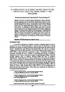
• Each vehicle route starts at vertex 0 and ends at vertex n + 1. Figure 1 shows a simple graphical model of the VRPTW and its solution. In this example, there are two routes, Route 1 with 4 customers and route 2 with 5 customers.
Figure 1: Example of a routing Solution for VRPTW The VRPTW model can be mathematically formulated as shown below:
Beatrice Ombuki, Brian J. Ross and Franklin Hanshar
min
XXX
cij xijk
7
(1) s.t.
k∈V i∈N j∈N
XX
=
1
∀i ∈ C
(2)
≤
q
∀k ∈ V
(3)
=
1
∀k ∈ V
(4)
=
0
∀h ∈ C, ∀k ∈ V
(5)
=
1
∀k ∈ V
(6)
≤
sjk
∀i ∈ N, ∀j ∈ N, ∀k ∈ V
(7)
oti ≤ sik ≤ cti
∀i ∈ N, ∀k ∈ V
( 8)
xijk ∈ {0, 1}
∀i ∈ N, ∀j ∈ N, ∀k ∈ V
(9)
xijk
k∈V j∈N
X
di
X
x0jk
X
xihk −
X
xi,n+1,k
i∈C
X
xijk
j∈N
j∈N
i∈N
X
xhjk
j∈N
i∈N
sik + tij − K(1 − xijk )
V = {1, 2, · · ·, k} vehicles C = {1, 2, · · ·, n} customer size 0, n + 1 depot N = {0, 1, · · ·, n, n + 1} node size di client i demand ai client i open time bi client i close time qk vehicle k capacity tij client i from j time sik client i take k service time The objective function (1) states that costs should be minimized. The constraint set (2) state that each customer must be visited exactly once by one vehicle, and constraint set (3) states that the vehicle capacity should not be exceeded. The next set of constraints (4), (5) and (6) give the flow constraints that ensure that each vehicle leaves the depot 0, departs from a customer it visited and finally returns to the depot, given by node n + 1. The nonlinear inequality (7) (which can be easily linearized, see [1]) states that a a vehicle K cannot arrive at j before sik + tij if it travels from from i to j. Constraint (8) ensures that time windows are observed and (9) gives the set of integrality constraints.
Beatrice Ombuki, Brian J. Ross and Franklin Hanshar
2.2
8
Multi-objective optimization and Pareto ranking
A multi-objective optimization problem (MOP) is one in which two or more objectives or parameters contribute to the overall result. These objectives often affect one another in complex, nonlinear ways. The challenge is to find a set of values for them which yields an optimization of the overall problem at hand. Evolutionary computation has been widely applied to MOP’s [34,35,36]. Their success resides in the general applicability of evolutionary algorithms in finding good solutions to problems with appropriate structure, and the adaptability of genetic representation and fitness evaluation towards problems in the MOP field. The Pareto ranking scheme has often been used in MOP applications of genetic algorithms [9]. It is easily incorporated into the fitness evaluation process within a genetic algorithm, by replacing the raw fitness scores with Pareto ranks. These ranks, to be defined below, stratify the population into preference categories. With it, lower ranks are preferable, and the individuals within rank 1 are the best in the current population. The idea of Pareto ranking is to preserve the independence of individual objectives. This is done by treating the current candidate solutions as stratified sets or ranks of possible solutions. The individuals in each rank set represent solutions that are in some sense incomparable with one another. Pareto ranking will only differentiate individuals that are clearly superior to others in all dimensions of the problem. This contrasts with a pure genetic algorithm’s attempt to assign a single fitness score to a MOP, perhaps as a weighted sum. Doing so essentially recasts the MOP as a single-objective problem. The difficulty with this is that this weighted sum necessitates the introduction of bias into both search performance and quality of solutions obtained. For many MOP’s, finding an effective weighting for the multiple dimensions is difficult and ad hoc, and often results in unsatisfactory performance and solutions. The following is based on a discussion in [36]. We assume that the MOP is a minimization problem, in which lower scores are preferred. Definition: Given a problem defined by a vector of objectives f~ = (f1 , ..., fk ) subject to appropriate problem constraints. Then vector ~u dominates ~v iff ∀i ∈ (1, ..., k) : ui ≤ vi ∧ ∃i ∈ (1, ..., k) : ui < vi This is denoted as ~u � ~v . The above definition says that a vector is dominated if and only if another vector exists which is better in at least 1 objective, and at least as good in the remaining objectives. Definition: A solution ~v is Pareto optimal if there is no other vector ~u in the search space that dominates ~v . Definition: For a given MOP, the Pareto optimal set P ∗ is the set of vectors ~vi such that ∀vi : ¬∃~u : ~u � ~vi .
Beatrice Ombuki, Brian J. Ross and Franklin Hanshar
9
Curr Rank := 1 N := (population size) m := N While N 6= 0 { /* process entire population */ For i := 1 to m { /* find members in current rank */ If ~vi is nondominated { rank(~vi ) := Curr Rank } } For i := 1 to m { /* remove ranked members from population */ if rank(~vi ) = Curr Rank { Remove ~vi from population N := N-1 } } Curr Rank := Curr Rank + 1 m := N } Figure 2: Pareto Ranking Algorithm
Definition: For a given MOP, the Pareto front is a subset of the Pareto optimal set. Many MOP’s will have a multitude of solutions in its Pareto optimal set. Therefore, in a successful run of a genetic algorithm, the Pareto front will be the set of solutions obtained. As mentioned earlier, a Pareto ranking scheme is incorporated into a genetic algorithm by replacing the chromosome fitnesses with Pareto ranks. These ranks are sequential integers values that represent the layers of stratification in the population obtained via dominance testing. Vectors assigned rank 1 are undominated, and inductively, those of rank i+1 are dominated by all vectors of ranks 1 through i. Figure 2 shows how a Pareto ranking can be computed for a set of vectors. First, the set of nondominated vectors in the population are assigned rank 1. These vectors are removed, and the remaining set of nondominated vectors are assigned rank 2. This is repeated until the entire population is ranked. Evolution then proceeds as usual, using the rank values as fitness scores. Note that Pareto ranks are relative measurements, and there is no concept of “best solution” using a rank score. Therefore, every generation in a run will have a rank 1 set. In order to determine whether an actual solution has been found, and that the run should be terminated, the raw fitness measurements need to be inspected.
Beatrice Ombuki, Brian J. Ross and Franklin Hanshar
3
Multi-Objective VRPTW
Genetic
Search
10
for
the
This section provides the details of the VRPTW representation, fitness evaluation, Pareto strategy and other GA parameters used. In the GA, each chromosome in the population pool is transformed into a cluster of routes. The chromosomes are then subjected to an iterative evolutionary process until a minimum possible number of route clusters is attained or the termination condition is met. The transformation process is achieved by our routing scheme described in sub-section 3.7. The evolutionary part is carried out as in ordinary GAs using crossover and selection operations on chromosomes. Tournament selection with elite retension is used to perform fitness-based selection of individuals for further evolutionary reproduction. A problem specific crossover operator that ensures solutions generated through genetic evolution are all feasible is also proposed. Hence, both checking of the constraints and repair mechanism can be avoided, thus resulting in increased efficiency. Figure 2 outlines the genetic routing system. procedure Genetic routing system; begin Read instance data(customer size and locations, time windows, capacity); Set GA parameters; Generate randomly an initial population, POP of size popSize; for gen = 1 to maxGen do Transform each chromosome into feasible network configuration by applying the routing scheme; Evaluate fitness of the individuals of POP; Rank the individuals of POP and select new population with the elite retaining strategy; Apply GA operators (crossover and mutation); endfor; end;
Figure 3: An outline of the genetic routing system
3.1
Chromosome Representation and Initial Population creation
In order to apply the GA to a particular problem, we need to select an internal string (chromosome) representation for the solution space. The choice of this component is one of the critical aspects to the success/failure of the GA for
Beatrice Ombuki, Brian J. Ross and Franklin Hanshar
11
a problem of interest. In our approach, a chromosome representing a network configuration is given by an integer string of length N, where N is the number of customers in a particular problem instance. A gene in a given chromosome indicates the original node number assigned to a customer, whilst the sequence of genes in the chromosome string dictates the order of visitation of customers. An example of a chromosome representing a solution for the network given in Figure 1 is as follows: 251478639 A chromosome string contains a sequence of routes, but no delimiter is used to indicate the beginning or end of a respective route in a given chromosome. However, the correspondence between a chromosome and the routes is further explained in Section 3.6. To generate the initial population, 90 percent of the population is created by random permutations of N customers nodes. The remaining 10 percentage is generate by a greedy procedure as follows: 1. Given a set of customers C of size N ; 2. Initialize an empty chromosome string l; 3. Randomly remove a customer ci ∈ C, else goto Step 8. 4. Add customer node ci to the chromosome string l; 5. Within an empirically decided Euclidean radius centered around centered around ci , choose the nearest customer cj , where cj 6∈ l; 6. If cj D.N.E then goto 3. 7. Append cj to l, and remove Cj from C; 8. Let ci = cj and goto 5. 9. If chromosome length = N , terminate, else goto 5;
3.2
Pareto fitness evaluation and other evaluation strategies
Once each chromosome has been transformed into a possible feasible network topology using the route clustering scheme given in Section 3.6, the fitness of each chromosome is determined. The chromosome fitness is evaluated according to two approaches: 1) weighted sum fitness function and 2) rank based upon Pareto ranking technique. Weighted sum method
Beatrice Ombuki, Brian J. Ross and Franklin Hanshar
12
Create initial population. Repeat until max. generation reached { For each chromosome i in population: Evaluate route, determining number of vehicles and cost. Determine Pareto rank. ⇒ ranki Apply GA to population, using ranki as fitness value. ⇒ new population }
⇒ (ni , ci )
Figure 4: GA with Pareto Ranking This method requires adding the problem objective functions together using weighted coefficients for each individual objective. That is, our multi-objective VRPTW is transformed into a single-objective optimization problem where the fitness of an individual F (x) is returned as: F itness
=
α· | V | +β ·
X
Dk
(1)
k∈V
Dk
=
XX
tij xijk
(2)
i∈N j∈N
α and β are weight parameters associated with the number of vehicles and the total distance traveled by vehicles respectively. The weight values of the parameters used in this function were established empirically and set at α = 100 and β = 0.001.
3.3
Pareto Ranking Procedure
A straight-forward MOP interpretation of the VRPTW is adopted. The two objectives are the number of vehicles and the total cost. They define two independent dimensions in a multi-objective fitness space. Thus, using the characterization of Section 2.1, each candidate VRPTW solution in the population has associated with it a vector ~v = (n, c), where n is the number of vehicles for that candidate solution, and c is the total cost. Unlike the weighted sum above, these two dimensions are retained as independent values, to be eventually used by the Pareto ranking procedure. Figure 4 shows how the Pareto ranking scheme of Figure 1 is incorporated with the genetic algorithm. Pareto ranking is applied to the (n, c) vectors of the population, essentially creating for the population a set of integral ranks ≥ 1. These ranks are then used by the GA as fitnesses for generating the next population. Note that the ranks themselves do not convey the quality of solutions, nor whether an optimal solution has been discovered. Each population, including the randomized initial population, is guaranteed to have a rank 1 set. This is not a disadvantage for general instances of the VRPTW anyway, since
Beatrice Ombuki, Brian J. Ross and Franklin Hanshar
13
there is no efficient means of knowing whether a candidate VRPTW solution is truly optimal.
3.4
Fitness based Selection
At every generation stage, we need to select parents for mating and reproduction. The tournament selection strategy with elite retaining model [9] is used to generate a new population. The tournament selection strategy is a fitness-based selection scheme that works as follows. A set of K individuals are randomly selected from the population. This is known as the tournament set. In this paper, the set size is taken to be 4. We also select a random number r, between 0 and 1. If r is less than 0.8 (0.8 set empirically), the fittest individual in the tournament set is then chosen as the one to be used for reproduction. Otherwise, any chromosome is chosen for reproduction from the tournament set. An elite model is incorporated to ensure that the best individual is carried on into the next generation. The advantage of the elitist method over traditional probabilistic reproduction is that it ensures that the current best solution from the previous generation is copied unaltered to the next generation. This means that the best solution produced by the overall best chromosome can never deteriorate from one generation to the next. In our GA, although the preceding fittest individual is passed unaltered to the next generation, it is forced to compete with the new fittest individual.
3.5
Recombination Phase
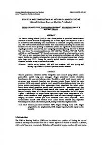
One of the unique and important aspects of the techniques involving genetic algorithms is the important role that recombination (traditionally, in the form of crossover operator) plays. In [11] we carried experiments where we established that two standard crossover operators: Uniform order crossover (UOX) [37] and Partially mapped Crossover (PMX) [37] are not suitable for VRPTW. We then introduced Route Crossover (RC) which is an improvement of the UOX. Experimental details showed that the RC outperforms UOX and PMX (see details of RC in [11]). Thus, in this work, we initially employed RC. While we established that the RC is better suited for VRPTW than well-known crossover operators, a weakness of the RC is that it is more suited for soft VRPTW where some conditions are relaxed. For example, when applying the RC occasionally results in some customers not being assigned to any vehicle. In this case, the chromosome resulting to unserviced customer(s) was simply penalized during the fitness evaluation stage. In this paper, we are dealing with hard VRPTW where all the constraints should be satisfied, hence we need a crossover operator that does not result in some customers being unserviced. This paper employs a problem specific crossover (Best Cost Route Crossover, BCRC) which aims at minimizing the number of vehicles and cost simultaneously while checking feasibility constraints. The dynamics of the proposed Best Cost Route Crossover are presented here.
Beatrice Ombuki, Brian J. Ross and Franklin Hanshar
Figure 5: Example Best Cost Route Crossover (BCRC) operator
14
Beatrice Ombuki, Brian J. Ross and Franklin Hanshar
15
Example 1 illustrates the creation of two offsprings, C1 and C2, from two parents, P1 and P2, using an arbitrary problem instance of customer size 9 for explanation purposes. RP1 and RP2 give corresponding set of routes associated with P1 and P2 respectively at the current generation. For examples, P1 has three routes (R1-R3) with respective customers, i.e., R1: 3 1 7, R2: 5 6 and R3: 4 2 8 9. As shown in Example 1a, from each parent, a route is chosen randomly. In this case, for P1, route R2 with customers 5 and 6 is chosen, while for P2, route R3 with customers 7 and 3 is picked. Next, for a given parent, the customers in the chosen route from the opposite parent are deleted. For example in 1a, for parent P1, customers 7 and 3 (which belonged to the randomly selected route in P2) is is deleted from P1 resulting in the upcoming child C1. Likewise customers 5 and 6 which belonged to a route in P1 are deleted from the routes in P2 resulting the upcoming C2. Since each chromosome should contain all the customer numbers (for a given VRPTW problem instance, the next step is to locate the best possible locations for the deleted customers in the corresponding children. As shown in 1b, the algorithm needs to re-insert customers 7 and 3 to child C1 and customers 5 and 6 should be inserted in child C2 respectively. Note that the choice of which customer to insert first is done randomly, i.e., in creating C1 for example, the order of insertion of 7 and 3 is done arbitrarily. In this case, customer 3 was first inserted in the best location found in C1 (as shown in 1b) before 7 was inserted as shown in 1c. An insertion point is said to be infeasible if it results to the routes either not meeting the vehicle capacity or time window constraints. The best insertion location is one that results in total minimum cost routes. In this example, customers 3 and 7 were both found to fit into route 3 of P1 as shown in 1c. Occasionally no feasible insertion point is found and a new route is started. For example, in creating C2, customer 6 could not be inserted in the current routes for P2 hence a new route was created.
3.6
Constrained Route Inversion mutation
Mutation aids a genetic algorithm to break free from fixation at any given point in the search space, and is used here in VRPTW for that very reason. Since mutation can be highly destructive of good schemas, each chromosome has a low probability of being mutated, in this research each chromosome has a 0.10 probability of being chosen for mutation. When utilizing mutation it may be best to introduce the smallest change in the chromosome as possible, especially in the VRPTW, where the time windows can easily be violated. We propose an adaptation of a simple widely used mutation, usually referred to as inversion [37]. In a simple use of inversion applied to the TSP, where the chromosome representation is simply a permutation of the order in which to visit each locale, two cut points are selected in the chromosome, and the genetic material between these two cuts points is reversed, for example given the TSP chromosome: 95178243
Beatrice Ombuki, Brian J. Ross and Franklin Hanshar
16
Two cut points are generated: 95|17824|3 And the genetic material is reversed between the cut points giving: 95428713 In this paper mutation is carried only in one randomly chosen route so as to minimize total route disruption. Maintaining route time window puts major constraints since the violation of individual customer time windows can segment that route into multiple routes. Thus we employ a constrained inversion, which is limited in length to 2-3 customers. Since an inversion of 2-customers is the smallest change one can make in a route (since it changes only two edges of the graph) we employ this type of mutation to aid search away from converging at local optima.
3.7
Routing Scheme
It is quite common among research for the VRPTW to route exhaustively in relation to vehicle capacity; that is, vehicles are filled with customers until capacity constraints disallow the addition of another customer. A worthy exception [32] attempts all feasible routing schemes, and chooses the routing scheme with the best cost. Our work used a two-phase routing scheme that transforms each of the chromosomes into a cluster of routes. In Phase 1, a vehicle must depart from the depot and the first gene of a chromosome indicates the first customer the vehicle is to service. A customer is appended to the current route in the order that he/she appears on the chromosome. The routing procedure takes into consideration that the vehicle capacity and time window constraints are not violated before adding a customer to the current route. A new route is initiated every time a customer is encountered that cannot be appended to the current route due to constraints violation. This process is continued until each customer has been assigned to exactly one route. In Phase 2, the last customer of each route ri , is relocated to become the first customer to route ri+1 . If this removal and insertion maintains feasibility for route ri+1 , and the sum of costs of r1 and ri+1 at Phase 2 is less than sum of costs of ri + ri+1 at Phase 1, the routing configuration at Phase 2 is accepted, otherwise the network topology before the Phase 2 (i.e., at Phase 1) is maintained.
4
Experimental Results and Comparisons
This section describes computational experiments carried out to investigate the performance of the proposed GA. In particular the experimental results shown here aim at showing two types of simulations: (i) where the VRPTW simulations consider only single objective where minimizing the number of vehicles is
Beatrice Ombuki, Brian J. Ross and Franklin Hanshar
17
given more weight over minimizing travel costs (ii) VRPTW is considered as a multi-objective problem (MOP) hence concurrently minimizing both number of vehicles and travel costs without a bias. The algorithm was coded in Java and run on an Intel Pentium IV 1.6 MHz PC with 512 MB memory. Our experimental results use the standard Solomon’s VRPTW benchmark problem instances available at [38]. Solomon’s data is clustered into six classes; C1, C2, R1, R2, RC1 and RC2. Problems in the C category means the problem is clustered, that is, customers are clustered either geographically or according to time windows. Problems in category R mean the customer locations are uniformly distributed whereas those in category RC imply hybrid problems with mixed characteristics from both C and R. Furthermore, for C1, R1 and RC1 problem sets, the time window is narrow for the depot, hence only a few customers can be served by one vehicle. Conversely, the remaining problem sets have wider time windows hence many customers can be served by main vehicles. See [39] for further descriptions of the Solomon’s problem sets. Unless otherwise stated, the results presented below are based on the following set of GA parameters: • population size = 300 • generation span = 350 • crossover rate = 0.80 • mutation rate = 0.10
4.1
Comparisons with best published results
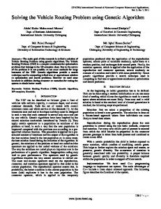
In Figures 4-6, we illustrate some of the network topologies obtained after running the GA for 350 generations. Figure 4 represents a data set where customers are clustered together and have a small time window. Figure 5 shows a data set where customers are also clustered but have a wider time window hence as expected, the network topology shows that one vehicle can serve more customers as opposed to Figure 6. On the other hand, Figure 6 shows customers that also have a small time window but the locations of customers is uniformly distributed. It should be noted that nodes in R1 category are much harder to solve than in C category. Due to space limitations we show only three network topologies here, however, the general behavior is representative of the respective data sets. Tables 1 and 2 present a summary of our results and compare them with the published solutions. Route costs are measured by average Euclidian distance. The column labeled Best Known gives the best known published solutions, column wGA gives the best solution where the VRPTW was interpreted as a single objective problem by using weighted sum fitness evaluation criterion. The columns labeled pGA Vehicles and pGA cost show the best solutions obtained when the VRPTW was interpreted as multi-objective optimization problem and the Pareto procedure was incorporated into our GA for fitness evaluation. The reported Pareto solutions in tables 1 and 2 are two examples from the Pareto
Beatrice Ombuki, Brian J. Ross and Franklin Hanshar
18
Figure 6: Network topology for 100 geographically clustered customers with a narrow time window. Test problem c101:[38]
Figure 7: Network topology for 100 geographically clustered customers with a wide time window. Test problem c201:[38]
Beatrice Ombuki, Brian J. Ross and Franklin Hanshar
19
Figure 8: Network topology for 100 uniformly distributed customers with a narrow time window. Test problem r108:[38] rank 1 set at the end of a run. pGA Vehicles solution is the rank 1 solution that has the minimal number of vehicles, while the pGA Cost value is the rank 1 solution with the minimal cost. Note that in experiments in which the difference in the number of vehicles in these two columns is ≥ 2, there are even further rank 1 solutions between these two extremes. We report only these two instances, however, to give an idea of the range of possible solutions returned by the Pareto MOP approach. Bolded figures in Tables 1 and 2 indicate an improvement on the best currently known results from literature (when considering either number of vehicles or cost). A tick on the other hand indicates that the solution we obtained is the same as the best known. The results obtained by our GA are quite good as compared to the best published results found in literature. The advantages of the efforts of interpreting the VRPTW as a MOP using Pareto ranking as opposed to the single objective using weighted sum can be established from the solution quality. When using the Pareto ranking, one has a choice of two (or more) solutions, depending on whether the user wants the best number of vehicles or best travel costs solutions. In some experiments, for example c101 in Table 1, there is a single Pareto solution that is optimal to the best known in both vehicle and distance dimensions. Other solutions, such as rc102, reduce the distance significantly, but at the expense of adding extra vehicles. In rc105, there are two reported solutions in the table that have better distance scores than the best known solution. However, both these solutions use 14 and 16 vehicles, which add 1 and 3 vehicles respectively to the 13 vehicles
Beatrice Ombuki, Brian J. Ross and Franklin Hanshar
20
used in the best known solution. Should distance (and hence time) be critical, then these alternate Pareto solutions are clearly preferable. Note that another Pareto solution with 15 vehicles may likely exist in rc105 as well, but it was not reported in the table. With weighted sum approach, there is only one solution which does not necessarily effectively serve the purpose of both objectives. Tables 3 and 4 give comparisons of our results with published results using GA (or hybrid GAs) in terms of average number of vehicles employed and average costs respectively (boldface are best solutions). Table 3 illustrates that our GAs (given by wGA and pGA) obtained better or similar average number of vehicles as compared to some of the well known published GA based methods for VRPTW. Except for [31] which is an hybrid strategy (incorporating GA, tabu search and simulated annealing), our wGA solution quality is better or very competitive with most of the other published work. The results of our multiple objective GA (given by pGA in Table 3) are equally competitive with other published work. Also in Table 4, it is shown that our multi-objective GA gives the best distances in almost all instances (see bold figures in Table 4) when considering costs. The corresponding average number of vehicles for the respective distances of the multi-objective GA is given in brackets under column pGA cost in Table 4. The corresponding average number of vehicles for the other published distances in Table 4 can be inferred from Table 3.
5
Concluding Remarks
This paper presented a multi-objective genetic algorithm approach to the vehicle routing problem with time windows. The solution quality of our GA is competitive with the best solutions reported for the VRPTW by other researchers. However, the most significant contribution of this paper is our interpretation of the VRP as a MOP. Our simple translation of the VRPTW into a MOP was surprisingly effective. Firstly, its performance was very good. Our results are competitive with other vehicle-biased results in the literature. Secondly, the Pareto scoring procedure precludes the need to experiment with weights as required in a weighted-sum approach. Poorly chosen weights result in unsatisfactory solutions, and only after considerably experimentation can effective weights be obtained for a specific instance of a VRPTW. Perhaps most significantly, our MOP interpretation of the VRPTW represents a philosophically view of the problem as the whole. When the VRPTW is viewed without bias towards number of vehicles or total cost, we are afforded with a more natural multi-modal perspective for this application problem. No unnecessary bias is introduced into the search. This is in stark contrast to most other work in VRP’s, in which the number of vehicles is given implicit priority, and consequently the scoring procedure must prioritize this dimension of the problem. We claim that there is no theoretical nor practical advantage to giving priority to the number of vehicles, perhaps other than having a common framework from which to compare different researcher’s results. Admittedly, there is an associated cost to having more vehicles, and the associated man-
Beatrice Ombuki, Brian J. Ross and Franklin Hanshar
21
Table 1: Solomon Benchmarks with narrow time windows: Comparison of our GAs with best published results Instance data c101 c102 c103 c104 c105 c106 c107 c108 c109 r101 r102 r103 r104 r105 r106 r107 r108 r109 r110 r111 r112 rc101 rc102 rc103 rc104 rc105 rc106 rc107 rc108
Best known 10 828.94 10 828.94 10 828.06 10 824.78 10 828.94 10 828.94 10 828.94 10 828.94 10 828.94 19 1650.8 17 1486.12 13 1292.68 9 1007.31 14 1377.11 12 1252.03 10 1104.66 9 963.99 11 1194.73 10 1124.4 10 1096.72 9 982.14 14 1696.94 12 1554.75 11 1261.67 10 1135.48 13 1633.72 11 1427.13 11 1230.48 10 1142.66
Ref. [21] [21] [21] [21] [13] [21] [21] [21] [13] [21] [21] [27] [27] [27] [21] [27] [27] [16] [20] [20] [8] [23] [23] [27] [27] [20] [25] [27] [23]
wGA √ √ √ √ √ √ √ √ √ √
1685.27 18 1523.10 √ 1348.28 10 1010.36 15 1427.72 √ 1273.62 11 1100.97 10 960.26 12 1211.81 11 1146.11 11 1132.51 10 985.99 15 1675.86 13 1536.04 12 1309.59 √ 1154.18 14 1623.33 12 1441.46 √ 1271.59 √
pGA Vehicles √ √ √
pGA cost √ √ √
10 825.65 √ √ √ √ √ √ 1690.28 √ 1513.74 14 1237.05 10 1020.87 √ 1415.13 13 1254.22 11 1100.52 10 975.34 12 1169.85 11 1112.21 11 1084.76 10 976.99 15 1636.92 14 1488.36 12 1306.42 √ 1140.45 14 1616.56 12 1454.61 12 1254.26 √ 1141.34
10 825.65 √ √ √ √ √ 20 1664.13 18 1487.07 1237.05 11 1010.24 15 1390.12 13 1254.22 1100.52 10 975.34 13 1166.09 11 1112.21 12 1079.82 10 976.99 15 1636.92 14 1488.36 12 1306.42 √ 1140.45 16 1590.25 13 1408.70 12 1254.26 12 1254.26
Beatrice Ombuki, Brian J. Ross and Franklin Hanshar
22
Table 2: Solomon Benchmarks with wide time windows: Comparison of our GAs with best published results Instance data c201 c202 c203 c204 c205 c206 c207 c208 r201 r202 r203 r204 r205 r206 r207 r208 r209 r210 r211 rc201 rc202 rc203 rc204 rc205 rc206 rc207 rc208
Best Ref. wGA pGA pGA known Sum Vehicles cost √ √ √ 3 591.56 [13] √ √ √ 3 591.56 [13] √ √ √ 3 591.17 [21] √ √ √ 3 590.60 [13] 596.55 596.55 596.55 √ √ √ 3 588.88 [13] √ √ √ 3 588.49 [13] √ √ √ 3 588.29 [21] √ √ √ 3 588.32 [21] √ √ 4 1252.37 [16] 1276.2 1268.44 7 1173.75 3 1191.7 [20] 41087.52 4 1112.59 5 1046.16 √ √ 3 942.64 [16] 952.52 989.11 5 890.50 2 849.62 [25] 3 766.92 3 760.82 3 760.82 √ √ 3 994.42 [20] 1036.08 1084.34 5 954.16 √ √ 3 912.97 [21] 921.32 919.73 4 889.39 2 914.39 [22] 3 821.32 3 825.07 4 822.90 √ 2 726.823 [8] 3 738.41 773.13 3 719.17 √ √ 3 909.86 [20] 928.93 971.70 5 874.95 √ √ 3 939.37 D[26] 983.77 985.38 5 930.42 2 910.09 [16] 3 786.23 3 833.76 4 761.10 √ √ 4 1406.94 [25] 1438.43 1423.73 7 1306.34 3 1377.089 [8] 4 1181.99 4 1183.88 8 1118.05 √ √ 3 1060.45 [16] 1078.38 1131.78 5 951.08 √ √ 3 798.46 [8] 810.15 806.44 4 796.14 √ √ 4 1302.42 [16] 1334.83 1352.39 7 1181.86 √ 3 1153.93 [20] 1203.7 4 1269.64 5 1080.50 √ √ 3 1062.05 [25] 1093.25 1140.23 5 982.58 √ √ 3 829.69 [20] 912.76 881.20 4 785.93
Table 3: Comparison of Average Number of Routes on the Solomon Benchmarks with other GA based published results. Set [18](95) [13](96) [31](99) [14](99) [12](01) [17](01) [32](01) [12](01) [10](03) wGA pGA (V) C1 10.0 10.0 10.0 10.0 10.0 10.1 10.1 10.0 10.0 10.0 10.0 C2 3.0 3.0 3.0 3.0 3.0 3.3 3.3 3.0 3.0 3.0 3.0 R1 12.8 12.6 12.3 12.6 12.6 13.2 14.4 12.6 12.8 12.7 12. 7 R2 3.2 3.0 3.0 3.1 3.2 5.0 5.6 3.2 3.0 3.2 3.1 RC1 12.5 12.1 12.0 12.1 12.8 13.5 14.6 12.8 13.0 12.3 12.5 RC2 3.4 3.4 3.4 3.4 3.8 5.0 7.0 3.8 3.7 3.4 3.5
Beatrice Ombuki, Brian J. Ross and Franklin Hanshar
23
Table 4: Relative Average Cost on the Solomon Benchmarks with other GA based published results Set C1 C2 R1 R2 RC1 RC2
[18](95) 892.11 749.13 1300.25 1124.28 1474.13 1411.13
[13](96) 838.11 590.00 1296.83 1117.64 1446.25 1368.13
[31](99) 830.89 640.86 1227.42 1005.00 1391.13 1173.38
[14](99) 857.64 624.31 1272.34 1053.65 1417.05 1256.80
[15](01) [17](01) [32](01) [12](01) [10](03) pGA cost 867.36 861 860.62 833.32 828.9 828.48 (10.0) 625.40 619 623.47 593.00 589.9 590.60 (3.0) 1369.97 1227 1314.79 1203.32 1242.7 1204.48 (13.1) 1193.6 980 1093.37 951.17 1016.4 893.03 (4.5) 1577.64 1427 1512.94 1382.06 1412.0 1370.79 (13) 1377.86 1123 1282.47 1132.79 1201.2 1025.31 (5.6)
power to drive them. However, there is also an associated cost to the additional fuel and time used in using fewer vehicles at longer distances to service clients. Furthermore, vehicle counts can be less important when vehicle and manpower costs are low if using for example bicycle couriers. By considering minimal cost (distance), we reduce energy consumption. Such ecological considerations are arguably of growing concern in a world of green house gases and a depleted ozone layer. In any case, the VRPTW is naturally multimodal, and neither dimension is fundamentally more important than the other from a theoretical perspective and even from a practical aspect, it is arguably debatable as to whether the optimization search should be biased towards minimizing the number of vehicles deployed as most current research work on VRPTW tends to do. Hence, as can be seen with our results, the MOP approach generates a set of equally valid VRPTW solutions. These solutions represent a range of possible answers, with different numbers of vehicles and costs. We leave it to the user to decide which kind of solution is preferable. Acknowledgment This research is supported by the Natural Sciences and Engineering Research Council of Canada Grant No. 249891-02. Special thanks to Mario Ventresca for his constructive input.
References [1] J. Desrosier, Y. Dumas, M. M. Solomon and F. Soumis, “Time constraint routing and scheduling,” In Handbooks in Operations Research and Management Science, Vol. 8: Network Routing, M.O. Ball, T/L Magnanti, C.L Monma, G.L. Nemhauser (eds.). Elsevier Science Publishers, Amsterdam, pp. 35-139, 1995. [2] J.F. Cordeau, G. Desaulniers, J. Desrosiers, M.M. Solomon, and F. Soumis, “The VRP with Time Windows. To Appear in The Vehicle Routing Problem,” Chapter 7, P. Toth and D. Vigo (eds), SIAM Monographs on Discrete Mathematics and Applications, 2001.
Beatrice Ombuki, Brian J. Ross and Franklin Hanshar
24
[3] O. Braysy, and M. Gendreau, “Vehicle Routing Problem with Time Windows, Part 1: Route Construction and Local Search Algorithms,” SINTEF Applied Mathematics Report, Department of Optimization, Norway, 2001. [4] O. Braysy and M. Gendreau, “Vehicle Routing Problem with Time Windows, Part II: Metaheuristics,” SINTEF Applied Mathematics Report, Department of Optimization, Norway, 2001. [5] M. R. Garey, and D. S. Johnson, Computers and Intractability, A Guide to The Theory of NP-Completeness, W. H. Freeman and Company, 1979. [6] J. K. Lenstra and A. H. G. Rinnooy Kan, “Complexity of Vehicle Routing Problem with Time Windows,” Networks, 11:221-227, 1981. [7] Niklas Kohl. “Exact Methods for Time Constrained Routing and Related Scheduling Problems,” PhD Thesis, Department of Mathematical Modeling, Technical University of Denmark, 1995. [8] L. M, Gambardella, E. Taillard and G. Agazzi, “MACS-VRPTW: A Multiple Ant Colony System for Vehicle Routing Problems with Time Windows,” In David Corne, Marco Dorigo, and Fred Glover, editors, New Ideas in Optimization, pp.63-76, McGraw-Hill, London, 1999. [9] D. E. Goldberg, Genetic Algorithms in Search, Optimization, and Machine Learning, Addison Wesley, 1989. [10] Kenny Q. Zhu. “A Diversity-controlling Adaptive Genetic Algorithm for the Vehicle Routing Problem with Time Windows,” Proceedings of the 15th IEEE International Conference on Tools for Artificial Intelligence (ICTAI 2003), pp.176-183, 2003. [11] B. Ombuki, M. Nakamura and O. Maeda, “A Hybrid Search based on Genetic Algorithms and Tabu Search for Vehicle Routing,”6th IASTED Intl. Conf. On Artificial Intelligence and Soft Computing (ASC 2002), pp. 176181. Banff, AB, ed. H Leung, ACTA Press, July 2002. [12] H. Wee Kit, J. Chin and A. Lim, “A Hybrid Genetic Algorithm for the Vehicle Routing Problem,” International Journal on Artificial Intelligence Tools, To appear. [13] J. Y. Potvin, S.Bengio, “The Vehicle Routing Problem with Time Windows- Part II: Genetic Search,” INFORMS Journal of Computing, 8: 165-172, 1996. [14] O. Braysy, “A New Genetic Algorithms for Vehicle Routing Problem with Time Windows Based on Hybridization of a Genetic Algorithm and Route Construction Heuristics,”, Proceedings of the University of Vaasa, Research Papers, 227, 1999.
Beatrice Ombuki, Brian J. Ross and Franklin Hanshar
25
[15] Kenny Q. Zhu, “A New Genetic Algorithm for VRPTW,” IC-AI 2000, Las Vegas, USA. [16] J. Homberger and H. Gehring. “Two Evolutionary Meta-heuristics for the vehicle routing problem with time windows,” INFORMS Journal on Computing, 37(3): 297-318, 1999. [17] K. C. Tan, L.L. Hay, O. Ke. “A Hybrid Genetic Algorithm for Solving Vehicle Routing Problems with Time Window Constraints,” Asia-Pacific Journal of Operational Research, Vol. 18, no.1, pp. 121-130, 2001. [18] S. Thangiah. “Vehicle Routing with Time windows using Genetic Algorithms,” In Applications Handbook of Genetic Algorithms: New Frontiers, Volume II, 253-277, CRC Press, Boca Raton, 1995. [19] W. C. Chiang and Russell, “Simulated Annealing Metaheuristic for the Vehicle Routing Problem with Time Windows,” Annals of Operations Research, 63:3-27, 1996. [20] L. M. Rousseau, M. Gendreau, and G. Peasant. “Using Constraint-based Operators to solve the Vehicle Routing Problem with Time Windows,” Journal of Heuristics, forthcoming. [21] Y. Rochat, E. D. Taillard. “Probabilistic Diversification and Intensification in Local Search for Vehicle Routing,” Journal of Heuristics 1: 147-167, 1995 [22] W. C. Chiang and Russell. “A Reactive Tabu Search Metaheuristic for the Vehicle Routing Problem with Time Windows,” INFORMS Journal on Computing, 9:417-430, 1997. [23] E. D. Taillard, P. Badeau, M. Gendreau, F. Gueritin, J. -Y Potvi, “A Tabu Search Heuristic for the Vehicle Routing Problem with Soft Time Windows,” Transportation Science, 31:170-186, 1997. [24] P. Badeau, M. Gendreau, F. Guertin, J.-Y. Potvin, E. D. Taillard, “A Parallel Tabu Search Heuristic for the Vehicle Routing Problem with Time Windows,” Transportation Research-C 5, 109-122, 1997. [25] J.F. Cordeau, G. Larporte and A Mercier. “A unified Tabu Search Heuristic for Vehicle Routing Problems with Time Windows,” Journal of the Operational Research Society, 52, 928-936, 2001. [26] B. De Backer, V. Furnon, P. Shaw, P.Kilby, and P. Prosser, “Solving Vehicle Routing Problems Using Constraint Programming and Metaheuristics, Journal of Heuristics, ” 6:501-523, 2000. [27] P. Shaw, “Using Constraint Programming and Local Search Methods to Solve Vehicle Routing Problems,” Proceedings of the Fourth International Conference on Principles and Practice of Constraint Programming (CP’98), M. Maher abd J.-F. Puget (eds.), Springer-Verlag, 417-431, 1998.
Beatrice Ombuki, Brian J. Ross and Franklin Hanshar
26
[28] H. Gehring and J. Homberger, “Parallelization of a Two-phased Metaheuristic for Routing Problems with Time Windows, ” Asia- Pacific Journal of Operational Research 18, 35-47, 2001. [29] J.Y. Potvin and J. M. Rousseau, “A Parallel Route Building Algorithm for the Vehicle Routing and Scheduling Problem with Time Windows,” European Journal of Operational Research, 66, 331-340, 1993. [30] W. C. Chiang and R. Russell, “Hybrid Heuristics for the Vehicle Routing Problem with Time Windows,” Transportation Science, Vol. 29, No. 2, 1995. [31] S.R. Thangiah, “A Hybrid Genetic Algorithms, Simulated Annealing and Tabu Search Heuristic for Vehicle Routing Problems with Time Windows,” Practical Handbook of Genetic Algorithms, Volume III: Complex Structures, L. Chambers (Ed.), CRC Press, 347-381, 1999. [32] K. C. Tan, L. H. Lee, Q. L. Zhu and K. Ou. “Heuristic methods for vehicle routing problem with time windows,”Artificial Intelligent in Engineering, pp. 281-295, Elsevier, 2001. [33] M. Dorigo, L. M. Gambardella, “Ant Colony System: A Cooperative Learning Approach to the Traveling Salesman Problem,” IEEE Transactions on Evolutionary Computation 1:53-66, 1997. [34] C. A. Coello Coello, D. A Van Veldhuizen, and G.B Lamont. Evolutionary Algorithms for Solving Multi-Objective Problems, Kluwer Academic Publishers, 2002. [35] C. M. Fonseca and P.J. Fleming. “An Overview of Evolutionary Algorithms in Multiobjective Optimization,” Evolutionary Computation, 3(1):116, 1995. [36] D. A Van Veldhuizen and G.B Lamont. “Multiobjective Evolutionary Algorithms: Analyzing the State-of-the-Art,” Evolutionary Computation, 8(2):125-147, 2000. [37] Z. Michalewicz, Genetic Algorithms + Data Structures = Evolution Programs (3ed.), Springer-Verlag, New York, 1998. [38] http://w.cba.neu.edu/ msolomon/problems.htm [39] M.M. Solomon. “Algorithms for the Vehicle Routing and Scheduling Problems with Time Window Constraints,” Operations Research, 35(2):254265,1987.