Multi-Objective Optimization Techniques for VLSI Circuits Fatemeh Kashfi, Safar Hatami, Massoud Pedram University of Southern California 3740 McClintock Ave, Los Angeles CA 90089 E-mail:
[email protected] Abstract The EDA design flows must be retooled to cope with the rapid increase in the number of operational modes and process corners for a VLSI circuit, which in turn results in different and sometimes conflicting design goals and requirements. Single-objective solutions to various design optimization problems, ranging from sizing and fanout optimization to technology mapping and cell placement, must hence be augmented to deal with this changing landscape. This paper starts off by presenting a variety of methods for providing analytical models for power and delay to be used in the optimization algorithms. The modeling includes non-convex and convex functional forms. Next, a class of robust and scalable methods for solving multi-objective optimization problems (MOP) in a digital circuit is presented. We present the results of a multiobjective (i.e., power dissipation and delay) gate (transistor) sizing optimization algorithm to demonstrate the effectiveness of our method. We set up the problem as a simultaneous, multi-objective optimization problem and solve it by using the Weighted Sum and Compromise Programming methods. After comparing these two methods, we present the Satisficing Trade-off Method (STOM) to find the most desirable operating point of a circuit.
Keywords Multi-objective optimization, Power, Delay, Pareto surface, Convexity, STOM
1. Introduction A multi-objective optimization problem (MOP) is the optimization of different objective functions simultaneously and reaching a solution that is the best in regard to all of the objective functions. Multi-objective optimization problems are present at different levels of VLSI circuit optimization. During the initial design, RTL/logic synthesis, and placement/routing steps, circuit designers typically wish to optimize a circuit with respect to its clock speed, power dissipation, and layout area at the same time. The optimization of a circuit for speed and power is nearly always conflicting i.e., higher speed leads to higher power dissipation and vice versa. If this optimization is done on the transistor or gate sizing of the circuit, finding the best sizing vector for both speed and power is a challenging task. This problem can also emerge in a circuit working under different supply voltage levels or clock frequencies, or even different die temperatures. AS discussed in the the power and speed This research was supported in part by a grant from the National Science Foundation.
1-xxxx-xxxx-4/10/$25.00 ©2010 IEEE
tradeoff case, multi-objective optimization techniques become important when optimization of different objective functions conflicts with each other. Multi-objective optimization is an important topic of research in science and engineering. There are many tutorials, review papers, and even text books written on this subject. Different aspects of nonlinear multi-objective optimization are defined in [1]. In [2] some advanced method for solving a MOP e.g., Fuzzy methods, interactive methods, and evolutionary algorithms are explained in details. Multi-objective optimization techniques have been applied for designing analog and digital circuits. Coello in [3] emphasizes Evolutionary Multi-objective Optimization and explains different methods using this technique. The author claims that aggregating objective functions by simply doing a weighted summation to produce a single function can be used for VLSI circuit optimization. In particular, the author shows that Vector Evaluated Genetic Search (GS), which is a modified version of the conventional GS in the selection step, is effective in designing some combinational circuits and multiplier-less IIR filters. The authors in [4] use multi-objective Genetic Algorithm optimization to design a low-power operational amplifier. The objective functions include gain, band-width, and power dissipation. In the field of digital circuit design, signal delay, chip area, and dynamic power dissipation are optimized with a design tool, called Multi-objective Gate Level Optimization (MOGLO) in [5]. Multi-objective optimization for VLSI interconnects is discussed in [6], where the objective functions to be simultaneously optimized are the metal widths, metal spaces, and metal thicknesses with the constraints on speed, area and power of the chip. This paper focuses on multi-objective optimization of power and delay, as an example of the two conflicting objective functions for VLSI circuits. The proposed methods can be applied for any other set of disagreeing functions to find the best (Pareto-optimal) operating point in today’s multi-mode multi-corner problems. First we propose different non-convex and convex models of power and delay and explain which ones are the most appropriate to be used in multi-objective optimization. In particular, we present three methods for solving a multi-objective problem. The first one is the Weighted Sum method which is the most popular technique for solving multi-objective optimization. Compromise Programming is the second method which is quite effective for convex functions. Finally a Satisficing Trade-off Method (STOM) based algorithm is presented for the optimization (Satisficing is a portmanteau of satisfy and 11th Int’l Symposium on Quality Electronic Design
suffice; it is a strategy that attempts to meet criteria for adequacy, rather than to try and find an optimal solution.) STOM can be used to find the best point when the designer is provided some goals for the objective functions. We will describe step by step how to find the best point of operation of a circuit in regard to multiple conflicting objective functions. The organization of the paper is as follows. In section 2 we present non-convex and convex modeling for power and delay. In section 3 we define MOP, Pareto optimal surface, methods of solving a multi-objective optimization problem, and our proposed approach. Section 4 presents the experimental results. Section 5 is the conclusion.
2. Power and Delay Modeling In this section, three different methods are proposed to model delay and power of a circuit. We will use these analytical models for multi-objective optimization.
2.1. Non-convex Modeling of Power and Delay The first modeling that we used is obtained by a second order polynomial interpolation of several sampling points of power and delay. We specified upper and lower bounds for the sizing vector elements and applied every permutation of the possible value of the sizing vector elements to a circuit analyzer (HSPICE) and then obtained the corresponding delay and power dissipation values for the circuit. Next by interpolation of the sampling points, we derived an analytical model for the circuit power dissipation and delay, which happens to be non-convex. The non-convex model of delay is formulated as follows: ∑
∑
(1)
⁄
∑∑
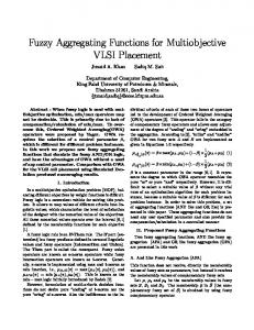
where n signifies the non-convexity of model, xi is the size of gate i. and i, i, and i are real-valued fitting coefficients. In the experimental results, the maximum error of the delay macromodel equation is 6% for every possible sizing vector value, while the mean and the variance are 1.5% and 1.2% respectively. The histogram of the modeling error is shown in Figure 1. Histogram of Error 25
Frequency(%)
20
15
10
5
0 0
1
2
3 Error bin
4
5
6
Figure 1 Histogram of error in non-convex delay modeling. The non-convex model of power dissipation is as follows:
Kashfi, Multi-Objective Optimization Techniques for ...
(2) where xi is the size of gate i. and i, i, i, and i are fitting coefficients and they are real numbers. The maximum error of this macromodel equation for power is 0.3% for every possible sizing vector value. 2.2. Convex Modeling of Power and Delay A multi-objective optimization is convex if all objective functions and the feasible region are convex. There are many algorithms that can solve a convex MOP but they face difficulty in solving non-convex MOP [1]. Definition (1): A function : is convex if for all , : 1 1 (3) 0 1 A set is convex if , implies that 1 for all 0 1. Delay and power dissipation can be modeled as convex functions of sizing vector elements too. We used posynomial functions for modeling circuit the power and delay values. These functions are convex when the variables have positive value [7]. Again the model is obtained by interpolation of the sampling points, and finding the best fitting coefficients. The convex delay modeling equation is as follows: (4) are positive where xi is the size of gate i, and , , , real numbers. The maximum error of this macromodel equation for every possible sizing vector elements in the specified range is 18%, while the mean and the variance are 3% and 5% respectively. The convex power modeling equation is as follows: (5) where xi is the size of gate i, and is positive real number. The maximum error of macromodel equation is 5%. By using convex modeling although we have less precise models, we can easily find the global optimum of the function during optimization. After finding the global optimum point using convex models, we narrow our search near the convex global optimum point and use more precise delay and power macromodel equations to find the actual optimum point of the functions. 3. Multi-Objective Optimization Problem Multi-objective optimization problem (MOP) can be formulated as follows: , ,…, 2 (6) . where fi is an objective function and : , ,… , is called the decision vector that the optimization is done on it. is the feasible region that is determined by the constraints on the MOP.
The goal is to minimize all objective functions simultaneously. We assume that there is no single solution that is optimal with respect to every objective function. The optimum single-objective solutions are at least partly conflicting with one another, and they can also be incommensurable, i.e., they may be expressed in very different units (μw of power dissipation vs. ns of delay). 3.1. Pareto Optimal Solution If the objective functions are conflicting, there is not a single solution that minimizes all the objective functions simultaneously. We are thus looking for a non-dominated solution in the sense that if we try to optimize one of the objective functions any further, the other objective function value(s) will degrade. This kind of optimality is called Pareto optimality [1]. Definition (2): A decision vector is Pareto optimal if there is no other decision vector such that for all 1, … , and for at least one index j. (Figure 2)
Figure 2. Pareto Optimal Set (a.k.a. the Pareto Surface). Mathematically a MOP is solved when the Pareto optimal set is reached. 3.2. Multi-objective Optimization Solution Methods MOP is usually solved by scalarization. It means that objective functions are combined in a way that at the end a single objective function will be optimized. As a single objective function can be optimized only to its local optimum, solving a MOP can also be ended in local Pareto optimal sets. If a MOP is convex then every locally Pareto optimal solution is also global Pareto optimal solution. Moving from decision vector in Pareto optimal solution to another needs trading off. Always there is a decision maker (the designer) with a better insight to the problem who decides which optimal decision vector to be chosen. A function : that represents the preference of the decision maker among all the objective function is called “Value Function”. In MOP the value function is assumed to be implicitly known [1]. A decision maker is needed to reach to a single solution for the problem. Based on the participation of the decision maker in different phases of the problem solving, methods of MOP is categorized in four categories. In the no-preference methods, the decision maker is not participated. In posteriori methods, decision maker will choose the desired answer among the Pareto optimal solutions at the end. In Priori methods, the preference and opinion of the decision maker is considered
Kashfi, Multi-Objective Optimization Techniques for ...
before the solving of the problem. In interactive methods, the decision maker is involved in every iteration of the optimization, and based on the new information will decide [1]. There are several methods for solving a MOP; here we explain three methods in detail. 3.2.1. Weighted Sum Method In the Weighted Sum (WS) method the weighted sum of the objective functions is minimized. The problem can be formulated as follows:
(7) 0
1
wi is the weight corresponds to objective function fi. wi’s are positive real numbers and are normalized. By perturbing the weights in the WS method we can find the Pareto Surface although some solution may be missed in non-convex functions [1]. WS is categorized as an a posteriori method. 3.2.2. Compromise Programming Method In this paper we also use an a priori method called Compromise Programming (CP) method for our MOP circuit optimization. In this method the distance between some reference point and the feasible objective region is minimized. Consider k objective functions of , ,…, to be optimized simultaneously. We assign the design references of , ,…, for the set of objective functions. These values can be equal to the minimum of each objective functions. The problem is formulated as follows: |
|
(8)
The vector of w specifies how much an objective function needs to get close to its reference. Sometimes some objective functions are relatively more important and the designer needs them to be much more optimized than the others. Therefore, by specifying larger wi to them, they will be encouraged to get closer to their references compared to others. The weighting vector also determines the direction of the search toward the optimum point in the feasible region. This method is robust and can be used in multi-objective optimization of a digital circuit. It is one of the simple and straightforward methods, and is very efficient in practice. In circuit optimization the designer can determine the optimum point (reference point) of each operating function (delay, power, etc). The preference of the decision maker is determined by the weights and the value of the references. If these values are chosen appropriately the Pareto optimal solution can be obtained by equation (8). However it is sometimes difficult to determine the best value of them. Moreover, the solution cannot be better than the references, even though they are
pessimistically underestimated. Note that the desirable solution can be obtained by adjusting the weight, and there is no positive correlation between the weight wi and the corresponding objective function [8]. 3.2.3. Satisficing Trade-off Method (STOM) Satisficing Trade-off Method (STOM) is an interactive method for getting a solution that a decision maker desires. After the Pareto optimal solution has been obtained it is presented to the decision maker. The objective functions are then classified in three classes, ones to be improved more, those which are accepted, and the objective functions that can be relaxed more. Based on this information aspiration levels (i.e., the objective function values that are satisfactory to the decision maker) will be specified. These aspiration levels will be developed interactively until the desired solution is obtained. In this method, in the first step, the range of each objective function is specified. For an objective function fi the maximum and minimum of it are shown by and . An aspiration level of is also specified for the objective function. The problem formulation in STOM method is as follows: (9) ,
1,2, … , ,
, 1⁄ This problem is usually solved for the small value of . If solution is satisfying the problem is solved, otherwise the decision maker will ask for another aspiration level [7][8]. 3.3. Proposed Approach Now we summarize the steps toward finding the best point of operation in regard to power and delay in VLSI circuits, which are also given in Figure 3. We can use either non-convex models of power and delay or convex models. Non-convex models have less error but they have a high chance of getting stuck in the local optimum points during the optimization. Convex models have more error but guarantee to lead to the global optimum points during the optimization. Furthermore, having generated analytical models for circuit power and delay parameters, we can also generate analytical equations for the gradients of the parameters of interest as well. Providing analytical gradient equations to the optimizer helps it achieve the global optimum point without suffering from the inaccuracies associated with the numerical computation of the gradient values during the optimization process. The impact of the gradient equation will be explained in section 4.1.1. By providing analytical gradient to the optimizer, the points on the Pareto surface can be reached more easily. Recall that these are the most optimum points based on Definition (2). After providing proper models and analytical gradient to the optimizer, we can optimize the circuit using the WS or CP method. As it will be explained in section 4.1.1 by using non-convex models, the WS method cannot result in all of the possible points on the Pareto surface; therefore, in this case the CP has an advantage over the WS method [8]. Kashfi, Multi-Objective Optimization Techniques for ...
If circuit power and delay parameters are of the same “value” to the designer, we should provide equal weights to them and do multi-objective optimization to find the best operating point of the circuit in regard to power and delay. Power and delay analytical modeling Convert non-convex to convex models Provide Analytical Gradient to the optimizer
Use WS or CP with the weights to obtain the result
YES
Are the weights provided? NO
Use equal weights and WS or CP to obtain the results
NO
Are the goals provided?
YES Use STOM to obtain the results
Figure 3. Power and delay multi-objective optimization. If on the other hand, the designer has a preference for lower delay over higher power dissipation (or vice versa), then the weights must be set so as to reflect this preference. Unfortunately it is hard to translate a designer’s preference for one or the other objective function into weights that yield the desired tradeoff behavior during multi-objective optimization process. In addition, sometimes there are objective function goals set by the designer. In this case we suggest that the designer uses STOM method, which is an interactive multi-objective programming technique based on aspiration levels. The aspiration levels are developed during the optimization until the desired solution is obtained. 4.Simulation Results We used combinational and sequential circuits to test the effectiveness of the multi-objective optimization algorithms which were defined in the previous sections. The combinational circuit is a Ladner-Fischer 10-bit carrylookahead adder shown in Figure 4 [9]. In the adder circuit, propagation delay of the critical path and power of the circuit are modeled as the function of gate sizing. Therefore the objective functions are delay and power and the elements of the decision vector are the sizing of the gates in the circuit.
methods for the non-convex modeling of power and delay are shown in Figure 6.
Figure 6. Simulation results for finding Pareto surface for non-convex modeling power and delay. (a) WS method (b) CP method.
Figure 4. 10-bit carry-lookahead adder. The sequential circuit is a True Single-Phase Clock (TSPC) flip flop [10]. In the TSPC FF, the Clk-to-Q delay and power dissipation are modeled as functions of transistor sizing. Therefore the two objective functions are Clk-to-Q delay and power dissipation and the elements of the decision vector are the sizing of the transistors in the circuit. The schematic of the circuit is shown in Figure 5.
Figure 5. TSPC Flip Flop 4.1. Multi-objective Power-Delay Optimization in the Circuit Now we explain how to find the best operating point of the circuit in regard to power and delay for the adder circuit. The method can be applied to other conflicting objective functions (area, delay, routing cost, etc.) and to other circuits. 4.1.1. Finding the Pareto Surface First we used non-convex (but more precise) models of power and delay and applied the WS and CP methods to combine the objective functions for optimization. For each weight combination (total of 100 weights) used to scaliarize the power and delay objective functions, we optimized the circuit for 100 initial sizing values. The simulation results for finding the Pareto surfaces reached for the WS and CP
Kashfi, Multi-Objective Optimization Techniques for ...
We see that for one step optimization, it is not guaranteed that we reach the global optimum points which are on the frontier of the obtained graph (lower left most points of the scatter plots i.e., the Pareto surface). There are two main reasons that, for each weight, we didn’t reach one point for all of the associated initial sizing vectors. The first is that both delay and power are nonconvex functions and they have local optimum besides their global optimum point. The second is that the optimizer calculates the gradients numerically. Therefore starting from one initial sizing solution, during the optimization iterations
Figure 7. Pareto surface for non-convex modeling of power and delay with analytical gradient provided. (a)WS method (b) CP method. it may not converge to the optimum points; rather it finds the point which is near the optimum points. By providing the analytical gradient for the optimizer, we directly reach the Pareto surfaces for the WS and CP methods as shown in Figure 7. Here again optimizations are done for 100 initial values for each weight (we used 100 weights). For each weight the optimizer found almost the same point for different initial vectors provided. We see that, in both scatter plots, the points in the right end of the Pareto surface have some spread and the optimizer did not give us one point (as the optimal point) for this weight. (There is the same behavior in the left end of the graph as well, but it is less severe.) This is where power has a weight of 1 and delay has a weight of
0. It means that the optimizer had to do single objective optimization. If we optimize the non-convex power for different initial points, we obtain the graph depicted in Figure 9(a), in which the x-axis corresponds to the number of the initial points (meaning, for example, that x=1 corresponds to the first set of sizing initial vector values supplied to the optimizer) and the y-axis corresponds to the optimized circuit power reached for that initial point of the optimization. The figure shows the optimization of the nonconvex power model, in which an analytical equation for the gradient of the circuit power dissipation function is also provided for the optimizer. We can see that the optimizer gets stuck in the local minimum in almost half of the optimizations done under different initial points. The single objective optimization on non-convex delay function is also got stuck in local optimums for some of the initial values of the sizing vector. Figure 7 also shows that the WS method has the drawback of not being able to find some points on the Pareto surface for the non-convex models (even for all the possible weights) while the CP method can find them.
As we can see there is only one value (global optimum point) for every random initial vector value for sizing. For convex modeling, both WS and CP can find all points on the Pareto surface. 4.1.3. STOM In this step we used equation (9) for the scalarization of our objective functions. The aspiration levels are the values of the objective function which have an equal percentage of degradation from their optimum values (obtained by single objective optimization.) After one step optimization if the desirable result is not obtained, the aspiration levels are revised by relaxing the objective function which has been over improved. With the proposed modeling of the delay and power (either convex or non-convex) and the convex shape of Pareto surface which can be obtained from the multi-objective optimization, up to 10% change in the aspiration levels can lead to the desirable results. Table 1 Simulation results for the adder circuit power Single-obj Single-obj nonMultiobjective ) Using of ( Delay Power convex Method Optimization gradient delay Optimization Optimization /convex ( ) w/o grad WS w grad nonconvex w/o grad CP w grad
Figure 8. Pareto surface for convex modeling of power and delay with analytical gradient provided. (a) WS method. (b) CP Method.
w/o grad WS w grad convex w/o grad CP w grad
Figure 9. (a) Non-convex power single optimization (b) Convex power single optimization. 4.1.2. Using Convex Modeling If we try to optimize the convex circuit power and delay equations with analytical gradient functions, we get the Pareto surfaces for the WS and CP methods depicted in Figure 8. We observe that we have much improved Pareto surface for convex models because now each weight has only one point as the optimal point. Single power optimization for convex modeling is shown in Figure 9(b). Kashfi, Multi-Objective Optimization Techniques for ...
Power
48.011
48.932
48.719
Delay
11.992
10.463
10.537
Power
47.924
48.908
48.657
Delay
12.533
10.279
10.389
Power
47.924
48.633
48.439
Delay
12.533
10.806
11.018
Power
48.019
48.908
48.148
Delay
12.808
10.279
11.317
Power
48.085
48.495
48.432
Delay
13.001
10.647
10.658
Power
47.809
48.451
48.335
Delay
13.642
10.306
10.381
Power
47.809
48.464
48.123
Delay
13.642
10.603
11.408
Power
47.809
48.451
48.102
Delay
13.642
10.306
10.791
4.1.4. Results In Table 1, for the adder optimization, the effect of convex and non-convex modeling and using of analytical gradient for single step multi-objective optimization are shown for WS and CP methods. In the table by single objective power optimization, we mean optimization of power and use of the obtained sizing vector for calculating delay. A similar definition applies to the single objective delay optimization. For non-convex modeling and when we do not use analytical gradient, single step optimization does not guarantee of reaching the best point of operation. We need to run the optimization algorithm for several initial sizing vectors to reach the best operating point in regard to power and delay. By using analytical gradient and convex modeling we can guarantee reaching of the best in a single step optimization.
Delay 1: WS/pow_opt 2:WS/del_opt 3:WS/multi 4:WS/grad/pow_opt 5:WS/grad/del_opt 6:WS/grad/multi 7:GA/pow_opt 8:GA/del_opt 9:GA/multi 10:GA/grad/pow_opt 11:GA/grad/del_opt
70 60 50 40 30 20 10 0 2
3
4
5
6
7
8
STOM
1
9 10 11 12 13
different optimization setups
power Single-obj Single-obj nonMultiobjective Using of ( ) Delay Power convex Method Optimization gradient delay Optimization Optimization /convex ( ) w/o grad WS w grad
nonconvex
w/o grad CP w grad w/o grad WS w grad convex w/o grad CP w grad
80
30 20 10 0 2
3
4
5
6
7
8
9
1: WS/pow_opt 2:WS/del_opt 3:WS/multi 4:WS/grad/pow_opt 5:WS/grad/del_opt 6:WS/grad/multi 7:GA/pow_opt 8:GA/del_opt 9:GA/multi 10:GA/grad/pow_opt 11:GA/grad/del_opt 10 11 12 13 12:GA/grad/multi
different optimization setups
STOM
1
15.21
Power
70.73
78.52
73.24
78.37
Delay
55.82
14.86
17.56
Power
72.709
79.17
75.118
Delay
53.858
15.11
16.4
Power
70.73
78.67
73.23
Delay
55.821
15
17.58
Power
70.709
77.677
74.571 16.549
Delay
56.858
14.6
Power
70.709
77.677
75.21
Delay
56.858
14.6
15.521
Power
71.898
78.634
74.411
Delay
53.548
14.998
17.01
Power
70.709
78.357
74.173
Delay
56.858
15
17.185
Power
100
Delay 80 60 40 20 0 1
2
3
4
5
6
7
8
9 10 11 12 13
1: WS/pow_opt 2:WS/del_opt 3:WS/multi 4:WS/grad/pow_opt 5:WS/grad/del_opt 6:WS/grad/multi 7:CP/pow_opt 8:CP/del_opt 9:CP/multi 10:CP/grad/pow_opt 11:CP/grad/del_opt 12:CP/grad/multi
(b) convex modeling Figure 10. Degradation from the optimum point of operation for power and delay for the adder circuit. Kashfi, Multi-Objective Optimization Techniques for ...
Power
Degradation from optimum point
Delay
Degradation from optimum point
90
40
15.192
(a) non-convex modeling Power
50
79.596
53.858
different optimization setups
100
60
72.709
Delay
5. Conclusion In this paper we considered multi-objective optimization in VLSI circuits. We presented different ways to provide
(a) non-convex modeling
70
Power
Delay 80 60 40 20 0 1
2
3
4
5
6
7
8
9
10 11 12 13
different optimization setups
STOM
80
Table 2 Simulation results for the Flip Flop circuit
STOM
Power
90
Degradation from optimum point
100
STOM, while more time consuming, can lead to the best results in which the obtained power and delay have only up to 30% degradation from the best power and best delay of the circuit (in both adder and flip flop).
Degradation from optimum point
Figure 10 shows the percent of the degradation from the best operating point of power and delay (which is obtained by single objective optimization and utilization of the analytical gradient). Multi-objective optimizations (number 3, 6, 9, 12) have better results in comparison with single objective optimizations. As we can see in both graphs multiobjective optimization with CP method and use of analytical gradient is the best solution in regard to both power and delay. In Figure 10 results of the STOM method are compared with the results obtained with single step optimization and shown in Table 1. Using the STOM, the designer is able to find the best desired point in which both power and delay has almost equal percent of degradation from their optimum points (this point is the best in regard to power and delay with equal weights corresponds to them.) Note that STOM is much more time consuming than aforesaid methods since we need to update aspiration levels in each step of optimization to find the best operating point. For the True Single-Phase Clock Flip Flop (TSPC FF), if we optimize the non-convex and convex models of power and delay simultaneously with the WS and CP methods, we will reach the same optimization results as the adder’s, although we changed the CMOS technology, the circuit topology and used transistor sizing instead of gate sizing. We conclude that for the proposed modeling of power and delay, we can reach an almost convex Pareto surface and we can generalize our analysis to other circuits. The simulation results are gathered in Table 2 and Figure 11. Again we can see that multi-objective optimization with CP method and using of analytical gradient is the best solution in regard to both power and delay.
1: WS/pow_opt 2:WS/del_opt 3:WS/multi 4:WS/grad/pow_opt 5:WS/grad/del_opt 6:WS/grad/multi 7:CP/pow_opt 8:CP/del_opt 9:CP/multi 10:CP/grad/pow_opt 11:CP/grad/del_opt 12:CP/grad/multi
(b) convex modeling Figure 11. Degradation from the optimum point of operation for power and delay for Flip Flop circuit.
analytical models of power and delay to be used by the optimizer. The models included convex and non-convex for the VLSI circuits. While convex model has more modeling error, it guarantees reaching the global optimum in a single step optimization. Non-convex model has much more chance to find the global optimum if the analytical gradient of the model is also provided to the optimizer instead of numerical gradient which is calculated point by point. Three methods for multi-objective optimization: Weighted Sum, Compromise Programming, and STOM were discussed. By providing a wide range of experimental results and analytical analysis we concluded that using convex models and analytical gradient with the CP method can reach to the best operating in a single step optimization. WS is less effective for solving MOP containing non-convex functions. If the designer has a specific desire point interactive STOM method is suggested. The proposed method can be applied on every conflicting operational function in VLSI circuits.
6. References [1] K. [2]
[3]
[4]
[5]
[6]
[7]
[8]
[9]
[10]
Miettinen, 1999: Nonlinear Multi-objective Optimization. Boston: Kluwer Academic Publishers. M. Ehrgott and X. Gandibleux. Multiple Criteria Optimization. State of the Art Annotated Bibliographic Surveys. Kluwer, 2002. C. A. Coello, “A short tutorial on evolutionary multiobjective optimization,” in Proc. 1st Int. Conf. Evolutionary Multi-Criterion Optimization, 2001, pp. 21–40. R. S. Zebulum, M. A. Pacheco, and M. Vellasco, “A multi-objective optimization methodology applied to the synthesis of low-power operational amplifiers,” in Proc. XIII Int. Conf. Microelectronics and Packaging, vol. 1, I. J. Chueiri and C. A. dos R. Filho, Eds. Brazilian Microelectronics Society, 1998, pp. 264–271. B. Hoppe, G. Neuendorf, D. Schmitt-Landsiedel, and W. Specks, “Optimization of high-speed CMOS logic circuits with analytical models for signal delay, chip area, and dynamic power dissipation,” IEEE Trans. Computer-Aided Design, vol. 9, pp. 236–247, Mar. 1990. M. B. Anand, H. Shibata, and M. Kakumu, “Multiobjective optimization of VLSI interconnect parameters,” IEEE Trans. Computer-Aided Design, vol. 17, no. 12, p. 1252, 1998 K. Kasamsetty, et. al., “A new class of convex functions for delay modeling and their application to the transistor sizing problem,” IEEE TCAD, vol. 19, no. 7, pp. 779– 788, July 2000. H. Nakayama, Y. Yun, M. Yoon. 2009: Sequential Approximate Multi-objective Optimization Using Computational Intelligence. Springer-Verlag Berlin Heidelberg. R.E. Ladner and M.J. Fischer, “Parallel prefix computation”, Journal of ACM, Vol. 27, No. 4, pp.831838, Oct. 1980. S. M. Kang and Y. Leblebici, CMOS Digital Integrated Circuits. New York: McGraw-Hill, 2002.
Kashfi, Multi-Objective Optimization Techniques for ...