Multi-Objective Testing Resource Allocation under Uncertainty - Unina

This article has been accepted for publication in a future issue of this journal, but has not been fully edited. Content may change prior to final publication. Citation information: DOI 10.1109/TEVC.2017.2691060, IEEE Transactions on Evolutionary Computation 1

Multi-Objective Testing Resource Allocation under Uncertainty Roberto Pietrantuono, Pasqualina Potena, Antonio Pecchia, Daniel Rodriguez, Stefano Russo, Luis Fernandez

Abstract—Testing resource allocation is the problem of planning the assignment of resources to testing activities of software components so as to achieve a target goal under given constraints. Existing methods build on Software Reliability Growth Models (SRGMs), aiming at maximizing reliability given time/cost constraints, or at minimizing cost given quality/time constraints. We formulate it as a multi-objective debug-aware and robust optimization problem under uncertainty of data, advancing the stateof-the-art in the following ways. Multi-objective optimization produces a set of solutions, allowing to evaluate alternative tradeoffs among reliability, cost and release time. Debug awareness relaxes the traditional assumptions of SRGMs – in particular the very unrealistic immediate repair of detected faults – and incorporates the bug assignment activity. Robustness provides solutions valid in spite of a degree of uncertainty on input parameters. We show results with a real-world case study.

I. I NTRODUCTION A. Motivations Testing is an essential activity to improve quality of software products, impacting their production cost and time-tomarket. Engineers have to judiciously manage testing resources, finding a trade-off among quality, cost and release time. The problem of testing resource allocation has been addressed in the software engineering literature mainly by formulating optimization models by means of Software Reliability Growth Models (SRGMs), able to describe the relation between test effort and reliability [27][35][46][59]. The way the optimization function and constraints are defined (e.g., cost minimization under reliability constraints, reliability maximization under cost/time constraints), and the SRGM modeling choices (e.g., multiple or single SRGM), have led to many models. While it is known that allocation choices impact jointly quality, cost and time, few proposals have addressed the problem in terms of multi-objective optimization [45][61][63]. Multi-objective models have no unique solution, and are valuable to generate the best set of alternatives, where trade-offs among contrasting objectives can be evaluated. Existing single- and multi-objective models have several assumptions/limitations that undermine their practical appliR. Pietrantuono and A. Pecchia are with the National Interuniversity Consortium for Informatics (CINI), Via Cinthia, 80126, Naples, Italy. E-mail: {roberto.pietrantuono, antonio.pecchia}@consorzio-cini.it. S. Russo is with the Department of Department of Electrical Engineering and Information Technology, Federico II University of Naples, Via Claudio 21, 80125 Naples, Italy. E-mail: {Stefano.Russo}@unina.it. P. Potena is with RISE SICS Väster˚as, Kopparbergsvägen 10, SE-722 13 Väster˚as, Sweden. E-mail: [email protected]. D. Rodriguez and L. Fernandez are with the Department of Computer Science, University of Alcalá, 28801 - Alcalá de Henares, Spain. E-mail: {daniel.rodriguezg, luis.fernandezs}@uah.es.

cation, often causing engineers to opt for easier – though nonquantitative – approaches. We identify major challenges in: • Impact of debugging. Most allocation models maximize fault detection, without accounting for the fault correction process. The actual quality of a software product depends on the number of corrected faults: debug unaware optimization can be remarkably misleading [8]. Real debugging consists of various sub-activities, which have a severe impact especially for large systems [7][23][38][41]. Debugging times and bugs’ priorities and assignment are crucial in allocation decisions; • Data uncertainty. Models rely on parameters (e.g., expected number of faults, fault detection rate, fault correction times) and on testing data (e.g., the operational profile) which are subject to non-negligible uncertainty. The quality-cost-schedule trade-off analysis may be strongly distorted by this uncertainty, as demonstrated by some work for single-objective optimization [28][30]. Even when testing parameters are estimated based on historical data, they only approximate real values; • Unrealistic assumptions. SRGMs rely on several assumptions: independent inter-failure times, no code change during testing, perfect and immediate repair. Moreover, many techniques choose a SRGM a priori, regardless of its suitability to the available data. Testing in real contexts is likely to generate data that partially violate the assumptions and may escape an a priori selected model; • Time-effort non-linearity. The relation between testing effort and time is generally non-linear [26][29]. This is considered almost only in single-objective models. We believe these issues are at the root of the gap between research results and industry practice in testing resource allocation. We aim to fill it by the following contributions. B. Contributions We define a multi-objective, debug-aware, robust and adaptive formulation of the testing resource allocation problem. Multi-objective denotes the ability to jointly consider: (i) quality – in terms of number of detected and corrected faults; (ii) cost – as expected cost of testing and faults correction; (iii) schedule – time to complete the testing activities. Debug-awareness refers to the inclusion of debugging in the model. This encompasses the bug fixing time distributions (removing the assumption of immediate debugging), as well as the impact of bug assignment. We leverage the bug history to (i) estimate the ability of debuggers to correct faults, and (ii) assess the expected fixing time for the software components

1089-778X (c) 2016 IEEE. Personal use is permitted, but republication/redistribution requires IEEE permission. See http://www.ieee.org/publications_standards/publications/rights/index.html for more information.


they work on1 . Besides testing resources, the model determines the best way to assign debuggers to functionalities to maximize the number of corrected faults at minimum time and cost. Robustness is the ability to produce solutions that are valid in spite of a given degree of uncertainty in the input parameters. We use Monte Carlo (MC) simulation to assess the robustness of a resource allocation solution under uncertainty. This approach allows eliciting and representing uncertainties as probability distributions, simulating the impact on the Pareto front of resource allocation solutions. Finally, the proposed formulation is independent from any specific type of SRGM. Adaptivity refers to the selection of the SRGM best fitting each system component, based on the analysis of its bug history or of online data [6]. The method works with any Non-Homogeneous Poisson Process (NHPP) model. The main contributions are: • Formulation of a multi-objective multiple-SRGM optimization model that addresses: (i) both the fault detection and correction processes; (ii) the testing time as function of the effort by means of testing effort functions (TEFs); (iii) the cost of testing and debugging. This allows exploring the trade-offs among typical testing objectives. Including TEFs in multi-objective formulations significantly improves resource allocation; • The inclusion of the debuggers scheduling problem, which supports accurate testing resource allocation. This is especially relevant in large software projects. • An approach to deal with the uncertainty of testing and debugging parameters that combines multi-objective evolutionary algorithms (MOEAs) and MC simulation. The former are used in a wide spectrum of reliabilityrelated optimization problems: resource management and task partition of grid systems, redundancy allocation, and reliability optimization [63]. MC methods are widely established for uncertainty analysis: examples are found in [37][51], where MC is used for handling parameter uncertainties in software architectures. Their combination allows reasoning in terms of “ranges” of potential solutions based on the ranges of input parameters; • The empirical analysis with a real-world industrial case study. The proposed method is the result of an industryacademia collaboration in the ICEBERG EU-project2 , investigating novel approaches to improve the understanding of software quality and its relation with cost. C. Organization The paper is organized as follows: Section II presents background notions. In Section III we present an overview of the testing resource allocation framework. Section IV deals with uncertainty; Section V presents the optimization model at the core of the approach. Section VI describes the method used in the empirical study. The results are presented in Section VII. Section VIII discusses threats to validity. Section IX overviews related work, while conclusions are presented in Section X. 1 Here

we refer to a component or module as an independently testable functionality. The terms are used as synonymous if not differently specified. 2 www.iceberg-sqa.eu.

II. BACKGROUND A. Modeling fault detection and correction through SRGMs Software Reliability Growth Models (SRGMs) are wellknown mathematical models of how reliability grows as software is improved by testing and debugging. They are built by fitting failure data collected during testing. We consider the most common class of parametric SRGMs, modeling the process as a NHPP. They are characterized by the mean value function (mvf ) m(t), which is the expectation of the cumulative number of defects N (t) detected by testing at time t: m(t) = E[N (t)]. The mvf is written as m(t) = a·F (t), where a is the expected total number of faults, and F (t) is a distribution function whose form depends on the fault detection process [19]. The variety of SRGMs includes: the seminal model by Goel and Okumoto in 1979 [18], describing fault detection by an exponential mvf ; the S-Shaped [60] and log-logistic [19] models, capturing increasing/decreasing behavior of the detection rate; the models derived from the statistical theory of extreme-value, based on the Gompertz SRGM [42]. Other models are available, accounting for needs emerged from real-world projects, e.g., non-negligible debugging times, imperfect debugging, multiple release points, nonlinear testing effort-time relation. A recent survey is in [33]. Most SRGMs used in testing resource allocation models (e.g., [25][26][27][29][35]) consider only the fault detection process, thus assuming the fault correction (i.e., debugging) being an immediate action. However, immediate debugging is very far from reality in today’s software systems: as software projects grow in size and complexity, the mean time to repair a fault is often very high, because of the complexity in managing the debugging workflow timely and correctly [7][23][41]. While many SRGMs refer exclusively to fault detection, we consider the combined modeling of fault detection and correction. In the literature, debug-aware SRGMs represent fault correction as a process following detection with a time-dependent behaviour [50][57]. Few proposals capture detection and correction together, wherein detection models are adjusted to consider several forms of the time-dependent fault correction [31], [34]. In this work, we leverage the framework proposed by Lo and Huang [34], where the correction mvf is derived from the detection mvf considering the equations of Xie et al. [57]. The framework is briefly explained hereafter. Let us first distinguish fault detection and correction by denoting with md (t) and mc (t) the two mean value functions, respectively. The mean number of faults detected in the time interval (t, t + t] is assumed to be proportional to the mean number of residual faults [34][50]. Similarly, the mean number of faults corrected in (t, t + t] is assumed to be proportional to the mean number of detected yet not corrected faults. This proportionality is expressed by the fault detection and fault correction rate per fault as functions of time, denoted with (t) and µ(t). The following relations hold: dmd (t) = (t)(a dt

md (t)), a > 0

dmc (t) = µ(t)(md (t) dt

mc (t))

(1) (2)



where a is the initially estimated number of faults in the system, (a md (t)) are the expected residual faults, and (md (t) mc (t)) are the yet uncorrected faults. In the case of constant detection rate per fault ( (t) = ), md (t) is the Goel-Okumoto exponential SRGM, md (t) = a[1 e t )]. The function mc (t) is modeled in relation to the fault detection SRGM and the fault correction time. It can be shown R t that, using Equations (1) and (2), and defining D(t) = 0 (s)ds Rt and C(t) = 0 µ(s)ds (i.e., the cumulative detection and correction rate, respectively), the cumulative number of detected and corrected faults are [34]: md (t) = a[1 e D(t) )] ⇣R ⌘ mc (t) = e C(t) 0t c(s)eC(s) md (s)ds = =e

C(t)

⇣R

t 0

ac(s)eC(s) [1

e

D(s) ]ds

⌘

(3)

(4)

For instance, if the detection process follows an exponential SRGM with parameter ( (t) = ), and the correction time is exponentially distributed with parameter (µ(t) = ), then: ✓

mc (t) = a 1 +

t

e

e

t

◆

(5)

In formulating the optimization model, we consider the so-computed fault correction for each functionality, in order to account for the real software quality increase occurring when a fault is actually corrected. The general expression in Equation (4) allows to avoid deciding a priori the SRGMs to adopt and/or the shape for the debugging time.

assuming md (0) = 0. The latter is replaced into Eq. 4 to obtain the effort-aware fault correction function, mc (t). We use this framework in the optimization model to describe the increase of quality as testing proceeds for each functionality. III. O PTIMAL TESTING RESOURCE ALLOCATION The objectives pursued by the allocation process are: (i) Fault Correction Objective (FCO), namely the expected number of corrected faults, to maximize; (ii) Testing Time Objective (TTO), namely the expected time to complete testing, to minimize; (iii) Testing/Debugging Cost Objective (TCO), namely the expected cost of testing and debugging, to minimize. The solution indicates the testing effort that must be devoted to each system functionality (or, equivalently, components), the binary assignment of debuggers to functionalities, and the hours each debuggers should spend on each functionalities. The phases of the process are now presented. A. SRGM Construction The first phase consists in inferring the functionality-level SRGMs in order to characterize the progression of testing activities. We do not assume any SRGM beforehand; the most suitable SRGM is inferred as follows: •

B. Modeling testing effort within SRGMs The previous framework assumes the effort spent for testing is proportional to the testing time spent. This is, in general, not the case as the testing effort does not necessarily vary linearly with time. In the literature, this has been typically modeled by so-called Testing Effort Functions (TEFs), which describe how effort varies with time. When a TEF is considered, the previous fault detection model (Eq. 1) is adjusted as: dmd (t) 1 ⇥ = (t)(a dt y(t)

md (t)), a > 0

(6)

where y(t) is the current testing-effort consumption at time t. The most common TEF, which was shown to well represent the usual trend of testing effort, is the logistic TEF [26], [25], [29] given by the following equation: Y (t) = p h

B

1 + Aexp[ ↵ht]

(7)

where B is the total amount of testing effort to be consumed; ↵ is the consumption rate of testing-effort expenditures; A is a constant; h is a structuring index (a large value models wellstructured software development processes); and y(t) = dYdt(t) . When considering the TEF, md (t) in Eq. (3) – and, correspondingly, in Eq. (4) – is replaced by the solution of Eq. (6), which depends on the chosen SRGM and TEF. For instance, considering the exponential SRGM, i.e., (t) = , and logistic TEF of Eq. (7), Equation (6) results in: md (t) = a(1

exp[ ( (Y (t)

Y (0))]), ↵ > 0

(8)

•

•

Data Gathering. Let f denote one in a set of functionalities F . At the beginning of the optimization process (t0 ), there are two possible cases: (i) historical testing data of f are available (e.g., from another system that includes f , or also from testing of a previous version of f ); (ii) no previous data exist. In the former case, the available fault correction times are used to fit SRGMs for functionality f , by using Equation 4. In the latter case, resources are initially allocated uniformly to functionalities: once testing starts, the incoming data are progressively used to fit SRGMs. The former case allows optimization before testing starts; however, it requires historical data. The latter case uses data gathered as testing proceeds, but the optimization can take place only when enough data are available. Dynamic allocation produces results more accurate and less sensitive to SRGMs assumptions violations, but it may be less useful if started late. Parameter Estimation. Data gathered for each functionality are fitted by means of all the SRGMs the tester wishes to try3 . Fitting of parameters for every SRGM is done via expectation-maximization (EM) [43]. SRGM selection. For each functionality, the obtained SRGMs are compared to select the best fitting one. We adopt a typical goodness-of-fit measure, i.e., the Akaike Information Criterion (AIC), already used successfully for SRGM selection in [42]. The SRGM with the lowest AIC value is preferred out of the set, denoting that the fitting incurs into the minimal information loss.

As a result of this SRGM selection, each system functionality is assigned the best fitting SRGM. 3 In our implementation, there are eight models available, namely: exponential, S-shaped, Weibull, log logistic, log normal, truncated logistic, truncated extreme-value max and truncated extreme-value min.



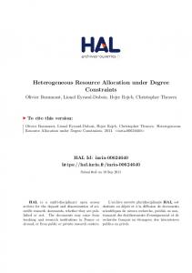
Fig. 1: High-level overview of the MOEA model solver. B. Parameters Specification In the second phase parameters are divided in deterministic (e.g., minimum reliability, available testing budget, hourly cost of a tester) and uncertain (e.g., SRGM parameters, average fixing time, usage profile), so as to establish the parameters to address by the proposed uncertainty handling approach. The specification of the parameters is detailed in Section IV. C. Robust Optimization In the third phase the optimization model is processed by a model solver, which implements a multi-objective evolutionary algorithm (MOEA). The solver starts with an initial population of candidate solutions (Figure 1), known as individuals in the MOEA terminology. At each iteration, operators, such as crossover and mutation, are used to generate new individuals. The fitness of an individual is evaluated by handling uncertain parameters through MC simulation: the parameters are sampled multiple times, thus generating more fitness values for each individual (MC loop in Figure 1). We associate to each individual an interval of fitness values (rather than a point solution), and we compare individuals according to interval comparison criteria. The interval solution reflects the variability of the optimal solution depending on the variability of uncertain parameters (uncertainty handling for robust optimization is detailed in Section IV.) The most promising individuals are selected by the MOEA, producing a new set of solutions (new population in Figure 1), until the MOEA stopping criteria are satisfied. IV. S OLUTION EVALUATION UNDER UNCERTAINTY Uncertainty is mainly dependent on the estimation of parameters either inferred from available data or that cannot be accurately evaluated when not enough information is available. Given a solution, the three objective functions (i.e., FCO, TTO, TCO) are evaluated by considering the uncertainty of parameters. In the following, we detail i) which are the uncertain parameters, ii) how individuals are compared to get robust solutions, and iii) the stopping criterion for MC runs. A. Specification of Uncertain Parameters The uncertain parameters are categorized as follows: Detection-specific parameters. They are related to the detection process of each functionality f . These are the parameters of the detection rate per remaining fault

•

function of the SRGM associated to f . Such parameters are encompassed by the D(t) function in Equation 4, and their estimation depends on (past or current) failure data (so, they are affected by uncertainty). • Correction-specific parameters, These are (i) the parameters of the correction rate per pending fault function, characterizing the debug-aware SRGM (C(t) parameters of Equation 4), and (ii) the average number of hours to fix a bug per functionality. Their estimation also depends on observed data (correction times). • Usage profile. The usage profile concerns how users interact with the system. It roughly expresses how much each functionality is expected to be used during operation. A widely adopted approach to express the user profile is the relative (percentage) frequency of invocation (e.g., calls rate) of each functionality, that can obtained by several approaches [46], [49]. These also are affected by uncertainty due to lack of knowledge about future usage. The values of these parameters are treated as samples of either continuous or discrete probability distributions. Distributions can be inferred by means of different approaches [51], such as: (i) using the source of variations, in the cases when the source of uncertainty is known and can be estimated; (ii) empirically, when a considerable amount of data regarding the parameter behaviour are available; (iii) approximation as a uniform distribution if no information is available, and (iv) as a discrete distribution, when parameters are discrete-valued. We use continuous uniform distributions (UD) for SRGMrelated fault detection parameters. Since a SRGM is built by fitting historical data, the ranges of the uniform distributions are set with the 95% confidence interval bounds of the parameters estimate. A discrete distribution over the set of functionalities is used for the usage profile values. Call rates are estimated by historical data about the usage of each functionality, if available; otherwise they are specified by a domain expert, or they are assigned an even probability if no estimate is available. Finally, in line with the literature, we use the exponential distribution for the fault correction SRGM (with the average correction rate as parameter), as it has been shown to well represent the debugging process [50]. In this case, the average correction rate µ(t) is constant, and is the reciprocal of the average number of hours to fix a bug (per functionality). The latter is estimated by querying data about bugs correction tracked in the company’s bug repository, as in [7][64][65], taking the median (or the mean, if the distribution is not skewed) of bug fixing times. If the information is not available, it should be assessed by a domain expert. B. Robust Solution Evaluation Samples are drawn from the above-mentioned distributions. They are used in the objective functions and constraints of the model to assess a candidate solution. The procedure is iterated N times – an iteration consisting of a MC run – until the desired accuracy is achieved. The output of a MC run leads to one possible fitness value of the candidate solution (i.e., the triple FCO, TTO and TCO). Given the N fitness values of the candidate solution, the robust values for the objective functions can be derived by



using two methods [37]. The former method consists in deriving a Probability Density Function (PDF) for each objective function and taking the robust objective as the value at a given confidence. However, this approach is computationally expensive; furthermore, prospective probability distributions need to be specified a priori. The alternative method leverages non-parametric or distribution-free statistical procedures. For each candidate solution and each objective, the method assesses descriptive statistics (e.g. percentiles, mean, variance or confidence bound) from the observed sample (consisting of the N MC runs). To capture the robustness of a candidate with different degree of tolerance, appropriate percentiles can be used as robust objectives. This method does not make any assumption on the probability distributions. We adopt the non-parametric method. Several options are available regarding the descriptive statistics. A conservative solution is to select the lower/upper bound, namely the 5th or 95th percentiles, depending on whether the objective is to maximize or minimize, respectively. This approximates the bounds of 95% confidence interval. Others percentiles could be selected (e.g., the 50th). For instance, if the objective is to maximize (such as in the case of FCO), we consider the lower bound as a robust solution (namely the 5th percentile of observed values); whereas, for TTO and TCO the 95th percentile is taken as robust solution. In this way, the Pareto-front concept is enhanced to express the robustness of a solution with respect to uncertainty of parameters: as a result, the notion of dominance used by the MOEA is adjusted accordingly. Given the minimization of a vector function f of a vector variable x (xk , k = 1, . . . , K), namely, minimization of f (x) = (f1 (x), . . . , fN (x)), subject to inequality and equality 0, j = 1, . . . , J and hm (x) = 0, m = constraints (gj (x) 1, . . . , M ), let us denote with ¯ f (x) = (f¯1 (x), . . . , f¯N (x)) the upper bound function vector, where f¯n (n 2 {1, . . . , N }) is the confidence upper bound of fn obtained from MC runs. Then, a solution vector u = {u1 , . . . , uK } dominates a solution vector f (u) is partially less v = {v1 , . . . , vK }, denoted by u v if ¯ than ¯ f (v), namely: 8n 2 {1, . . . , N }, f¯n (u)  f¯n (v) ^ 9n 2 {1, . . . , N }: f¯n (u) < f¯n (v). On this basis, the output Pareto front can also account for parameters uncertainty. C. Stopping Criterion We address the issue of selecting the number N of MC runs (i.e., the sample size) that should be performed to have an accurate estimate for each candidate solution. We use a dynamic stopping criterion [37][48] to (i) monitor the accuracy of the value to estimate (e.g., number of faults corrected) and (ii) automatically stop the MC step when the number of runs is enough to meet a predefined error threshold. For instance, let us consider the FCO objective and denote with f1 the value of the objective after one MC run. Further runs of the MC simulation will likely provide different values of the objective, due to the parameters’ values taken at each run, i.e., F =f1 , f2 , . . . fN . The goal is to establish the number of runs N to obtain an estimate of the desired percentile of the set F , i.e., fˆperc . The procedure is as follows: • A minimum of k MC runs are performed. After k repetitions, the desired percentile is estimated on the

•

•

collected set (f1 , . . . , fk ), obtaining the first estimate of the percentile, fˆperc1 . As the number of runs increases beyond k, further estimates are obtained, considering the increasing number of observations, i.e.: fˆperc2 from f1 , . . . , fk+1 ; fˆperc3 from f1 , . . . , fk+2 , and so on. The variation of the estimate is monitored over a sliding windows of size k. The last k estimates are considered: {fˆpercj , fˆpercj+1 , . . . fˆpercj+k }. The statistical significance for the last k estimates is: 2z(1 ↵/2) p e= k

r

2 fˆperc

⇣

fˆperc

¯ fˆperc

⌘2

(9)

where e is the relative error, fˆperc is the average of 2 last k estimates, fˆperc is the mean-square of the last k estimates, z is the normal distribution evaluated at the desired significance level ↵. The relative error e is checked against a predefined tolerance level (set to 0.01 in this study): MC runs are stopped when the error is below this level, as the desired accuracy is achieved. MC runs not satisfying some constraint of the model (e.g., because of values of uncertain parameters causing the constraint violation) are discarded and not counted as run. V. O PTIMIZATION MODEL FORMULATION The formulation aimed at minimizing the three objective functions (-F CO, T T O, T CO), under reliability and testing budget constraints, uses the notations listed in Table I. A. Assumptions The following assumptions are made, similarly as in related research [63][30][11][61][26]. • Functionalities are independently testable; • Usual SRGMs assumptions, namely: fault detection and removal can be modeled as a NHPP; the mean number of faults detected in the (t, t + t ) is proportional to the mean number of remaining faults; interfailure times are independent. SRGMs have been demonstrated to provide accurate predictions even when these assumptions are partially violated [1]; • The relation between testing effort and testing time can be modeled by a TEF [29]; • Debugger manpower is available to independently fix bugs in system functionalities. B. Model parameters The main parameters given as input to the model are: • The initial time t0 : it is the time the tester decides to run the algorithm. As described in Section III, t0 can denote the beginning of testing (when historical data are used to build the SRGMs; t0 = 0), or any time during testing (when online testing data are used; t0 > 0). In the latter case, allocation can be run repeatedly during testing (i.e., dynamic allocation); we refer to t0 as (re-)iteration time. • Fd&c (t0 )k is the number of faults detected and corrected in functionality k at time t0 (Fd&c (t0 )k = 0 if t0 = 0). • SRGMs for each functionality are characterized by k (t), and µk (t) (cf. with Equations 1 and 2), i.e., the detection



TABLE I: Notations adopted in the formulation of the multi-objective optimization Symbol K ak k

R Fd&c (t0 )k xk d Ndk Yk (t) B C1⇤ ↵ ⇤

k d

yk (t) h mdk (t0 + tk ) mck (t0 + tk ) C3⇤

Description Symbol Description Number of system functionalities k System functionality index Expected number of initial faults in the functionality k !k Probability the functionality k will be invoked Average number of hours required for fixing a bug of the functionality k t0 Time at which the resource allocation model is run Minimum threshold given to the reliability on demand of the system Y0 Testing effort (measured in man-hours) already spent at time t0 Number of faults (of the functionality k) detected and corrected at t0 D Total number of debuggers Debugger d used/not used to fix bugs of the functionality k (i.e., 1/0) d Debugger index Time assigned to the debugger d for testing the k-th functionality (hours) tk Calendar testing time devoted to test the functionality k (hours) Cumulative testing effort devoted to functionality k in (0, t] (man-hours) Fault detection rate per undetected fault for the functionality k k (t) Total amount of testing-effort available for consumption (man-hours) A Constant parameter in the logistic TEF ⇤ Average cost per man-day to correct a bug during testing C2 Average cost per man-day to correct a bug in operational use Consumption rate of testing-effort expenditures in the logistic TEF Expected failure intensity function for k at testing time t k (t) Maximum threshold given to failure intensity of the system after test µk (t) Fault correction rate per detected but uncorrected fault for k Average number of hours in a day that the debugger d can work to fix bugs of the functionality k (# of hours over 24h) Instantaneous testing-effort at time t for the functionality k, estimated by a generalized logistic testing-effort function (man-hours) Structuring index in the logistic TEF whose value is larger for better structured software development efforts Expected cumulative number of faults detected in functionality k at testing time t0 + tk Expected cumulative number of faults corrected in functionality k at testing time t0 + tk Average cost of testing a functionality per unit testing-effort expenditure, expressed in cost of a man-day

and correction rate per fault. They are related to D(t) and C(t), and consequently to md (t) and mc (t) functions used in the objective functions. • The k parameter is the average number of hours required to fix a bug for functionality k 4 . Recall that, being the correction time assumed exponential, the rate µk (t)= µk is estimated as µk = 1/ k . • !k is the call rate, namely the probability that the k-th functionality will be invoked: !k 0, 8k = 1 . . . K, and: P K k=1 !k = 1. Note that parameters of k (t), µk (t) and !k , k are the uncertain parameters (Section IV-A). • ↵, h, B, A are the parameters of the logistic testing effort function (Equation 7), which is used to explain how testing effort varies in function of calendar time. They were discussed in Section II. k • d is the processing capacity of debugger d with respect to functionality k. It represents the working rate of the debugger, expressed as average number of hours per day that debugger d is allowed to work on functionality k. ⇤ ⇤ ⇤ • C1 , C2 , C3 are the cost parameters used in the costrelated objective function (TCO). They are: (i) C1⇤ , the cost per man-day to correct a bug during testing; (ii) C2⇤ , the cost per man-day to correct a bug during operational use (typically C2⇤ > C1⇤ [5]); (iii) C3⇤ , the cost per testingeffort expenditure unit (e.g., man-hour or man-day) to test a functionality (i.e., hourly or daily cost of a tester). Note that SRGM parameters (parameters of k (t), µk (t), ↵, h and A) are estimated by fitting (historical or online) testing data as discussed in Section III; !k and k are estimated by historical data, design information or expert judgment (cf. Section IV-A); debuggers capacity dk , cost parameters Ci⇤ and the budget B are provided as input by the tester. C. Variables The decision variables of the model are: • Yk (1kK) variables are used to suggest the amount of testing effort (in man-hours) to perform on functionality k; Yk depends on the calendar testing time tk devoted to test functionality k. The relationship between testing effort and time is modeled by the logistic TEF (Equation 4 For

k ),

simplicity, we assume that this time, for a given functionality k (i.e., is the same for each debugger d working on that functionality.

7): the amount of spent testing time corresponds to tk = F 1 (Yk ) hours, where F 1 is the inverse of the TEF. k k • xd (1dD, kK) and Nd (1dD, 1kK) variables are used to regulate the assignment of debugger d to functionality k. Thus, the fault correction process is modeled as function of available debuggers. Specifically, xkd = 1 if debugger d is scheduled on functionality k, and 0 otherwise. Ndk is the time (in hours) assigned to debugger d to work on functionality k in (t0 ,tk ]. A solution consists of: a vector Y of Yk values, with the optimal testing effort per functionality; a matrix X of xkd values, assigning debuggers to functionalities; a matrix N of Ndk values, with number of debuggers’ hours per functionality. D. Constraints The most relevant constraints are the following ones: 1.

PD

d=1

2. Ndk  3.

⇢

Ndk tk

k d

k (mdk (t0

xkd = 1 iff Deb. d to be assigned to k; 8k = 1 . . . K, 8d = 1 . . . D xkd = 0 iff Deb. d not to be assigned to k; 8k = 1 . . . K, 8d = 1 . . . D mdk (t0 )  ak

PK

Yk  B 8k = 1 . . . K

PK

!k ·

k=1

6. Yk  B(1 7.

mdk (t0 )) 8k = 1 . . . K

· xkd 8k = 1 . . . K, 8d = 1 . . . D

4. mdk (t0 + tk ) 5.

+ tk )

k=1

QD

d=1 (1

k (tk )



Fd&c (t0 )k 8k = 1 . . . K

xkd )) 8k = 1 . . . K ⇤

They are to be interpreted as follows: • For each functionality k, faults detected in the interval (t0 ,tk ] must be fixed. Equation 1 represents this constraint. The total time (in hours) assigned to debuggers on functionality k must be greater or equal than the expected time to correct the detected bugs (estimated as mean fixing time per bug multiplied by the expected number of bugs that will be detected if functionality k is tested for a time tk ). • The bug correction process is modeled as a function of (i) the amount of time (in hours) required to fix the bugs detected and (ii) the working time of debuggers. The waiting queues are modeled by a constraint on the capacity of debuggers. Equation 2 represents this constraint.



For each functionality k, the load of debugger d caused by the assignment of bugs is limited by a function of the processing capacity of debugger d (i.e., dk ). Ndk is greater than 0 only if: i) the debugger d is allocated to functionality k (xkd = 1), ii) a non-zero testing time tk is allocated to functionality k (tk > 0), and, from constraint 1, iii) at least one bug is expected to be detected during the assigned time tk (i.e., mdk (t0 + tk ) > mdk (t0 )), assuming dk > 0 and k > 0. • Equation 3 represents (possible) constraints, which can be defined for debuggers that must or cannot be assigned to functionalities for some reasons, e.g., due to the debugger’s skill level or expertise area. In these cases, the corresponding variable xkd is forced to be 1 or 0. Note that, to solve incompatibilities or dependencies among debuggers and/or functionalities, due, for instance, to human factors or functionality characteristics, additional constraints can be added. For example, x12  x23 means that if debugger 2 is scheduled on functionality 1, then debugger 3 must be scheduled on functionality 2. • Equation 4 states that the expected number of faults detected in (t0 , tk ] (where tk = F 1 (Yk ) is the time devoted to test functionality k) cannot be greater than the expected number of residual fault of functionality k. • Equation 5 is a constraint on the maximum effort that can be allocated. The sum of efforts cannot exceed the maximum available budget B (expressed in man-hours). • If there are no available debuggers for functionality k, then the effort Yk allocated to it must be zero (as detected bugs would not be corrected). In other words, if functionality k receives a certain amount of testing effort, one or more debuggers must be assigned to functionality k. Equation 6 represents this constraint. • Equation 7 is the constraint on a maximum desired failure intensity at the end of testing T . Failure intensity k (tk ) of a functionality k is estimated through its SRGM as the derivative of md (t). A maximum failure intensity threshold ⇤ is given as input. In an average case, like the one we assume, this constraint is expressed by Equation 7. In the worst case, all functionalities could be required to satisfy the failure intensity constraint, and the constraint would be: maxk=1...K ( k (tk ))  ⇤ . Notice that this constraint can be referred to as reliability constraint, since failure intensity at the end of testing is related to reliability: R(t|T ) = exp[ (T ) · t], where T is the release time [46]. Further system-specific constraints could be introduced based on specific needs, but at the expense of higher complexity and less understandability. E. Multi-Objective Function 1) Fault correction process’ Effectiveness Objective (FCO). The objective is to maximize the predicted number of corrected faults at the end of testing. The prediction is carried out by the debug-aware SRGMs per functionality. F CO =

K X

k=1

mck (t0 + tk )

(10)

where (taking Equation 4 and Yk = T EF (tk )): mck (t0 + tk ) = e⇣ Ck (t0 +tk ) R · tt0 +tk ak c(s)eC(s) (1

⌘ exp[ (Dk (Yk (s))])ds . (11)

0

The expression can be instantiated for any detection and correction rates (D(t) and C(t)) and TEF relating t to Y . For instance, in the case of exponential detection and correction process ( (t) = , µ(t) = µ), it becomes: mck (t0 + tk ) = e⇣ µk ·(t0 +tk ) R · tt0 +tk ak · µk eµk ·s (1 0

exp[

k Yk (s)])ds

⌘

.

The expected number of faults detected and corrected depends on: (i) the fault detection rate, related to the testing effort Yk and time tk (through the TEF); (ii) the availability of sufficient debuggers (hours), regulated by Ndk and xkd variables, for the correction of detected faults at the rate expressed by Ck (t). 2) Testing Time Objective (TTO) The relationship between testing effort and time is typically modeled by the TEF. For a generic TEF F , we could write: tk = F 1 (Yk ). Assuming the TEF being modeled by the generalized logistic testing-effort [29] (Equation 7), testing time for functionality k is: tk =

1 · ln ↵⇤h

( YB )h k

A

1

!!

(12)

where parameters are as described in Section II. Since functionalities are assumed to be tested independently, TTO is the time minimization for testing the K functionalities: TTO =

(13)

min tk

k=1···K

3) Testing-effort Cost Objective (TCO) The third objective concerns with the minimization of cost, which is a measure related to the effort spent but that goes beyond it. In agreement with [25], [58], the cost of testing-effort expenditures during software development and testing, and the cost of correcting errors before and after release, can be expressed as: Costk (t)

= C1⇤ · ( k /24) · mck (t) +C2⇤ +C3⇤

· ( k /24) · (mdk (1)

(14) mck (t))

· (Yk /24)

where: (i) C1⇤ · ( k /24) is the cost to correct a bug during testing; (ii) C2⇤ · ( k /24) is the cost to correct a bug in operational use (typically C2⇤ > C1⇤ [5]); and (iii) C3⇤ is the cost of testing per unit testing-effort expenditure, expressed in cost of a man-day (for a tester). The TCO is the minimization of total cost over all the functionalities: T CO =

K X

Costk (Yk )

(15)

k=1

The three objectives to minimize are thus: min(-F CO, T T O, T CO), under the specified constraints.



VI. E XPERIMENTATION We design an empirical study to experiment the method. The addressed research questions are presented, followed by the industrial case study description and the experimental setup. A. Research questions •

•

•

•

RQ1. Multi-objective optimization. A multi-objective optimization problem is formulated and solved by various metaheuristics. We formulate these questions to assess the goodness of proposed solutions: – RQ1.1. Validation. How does the proposed approach perform compared to random search? This is a typical question performed as a preliminary “sanity check”, since any intelligent search technique is expected to outperform random search unless there is something wrong in the formulation [16]. – RQ1.2 Comparison of metaheuristics. Which of the considered multi-objective evolutionary algorithms (MOEAs) yields the best solution? This question focuses on the comparison among common MOEAs according to performance metrics regarding the goodness of the provided Pareto solutions. RQ2. Uncertainty analysis. The proposed approach deals with parameter uncertainty: what is the effect of explicitly considering the uncertainty of parameters? This question aims at evaluating to what extent embedding the MC simulations into the search technique provides robust solutions and at what computational expense. RQ3. Sensitivity to debugging. The proposed approach considers the debugging process: how does the optimal solution vary when considering debugging in the model? Differently from existing allocation models, our model is based on the fault correction process. This question aims at evaluating solutions computed by considering the bug assignment activity against solutions not explicitly incorporating bug assignment, under various configurations. RQ4. Scalability: How does the performance of our approach change while varying problem size? With the selected case study, we show to what extent the process is fast enough to analyze a real testing effort allocation decision problem whose size and complexity is similar to those of other published large-scale/industrial testing effort allocation problems (e.g., [6] and [63]).

B. Case study We consider a real-world issue tracking system of a Customer Relationship Management (CRM) software of a multinational company operating in the healthcare sector. Data have been made available within the ICEBERG European Project by ASSIOMA.NET, an IT company involved in the development of the CRM5 . The system has a layered architecture, with a Front-end layer, a Backend layer and a Database, made interoperable through an Enterprise Application Integration (EAI) layer. It provides typical CRM functionalities: sales management, customer folder, agenda, inventory, supplying, 5 An anonymized version of the dataset we used in this paper is available on demand for research purposes.

payments, user profiling, and various reporting tools. Collected issue records span a period of 2 years and a half, from September 2012 to January 2014. A total of 612 software faults collected during testing are considered. Once faults are detected, they undergo a debugging process: when an issue is opened, it becomes new and it is enqueued, waiting to be processed (published state); once an issue starts to be processed (in study), it is assigned (launched) to a developer and, once completed, it can be assigned to another developer for further processing, if needed. Then, the amendment is tested, delivered, and finally closed. Detection and correction times are tracked in the issue tracker The Time To Repair (TTR) a fault is the time to transit from the new state to the closed state. The TTR distribution is highly skewed in our data: medians of TTR values in lieu of means are considered to represent the average TTR per functionality. C. Experiment settings 1) Setting for MOEAs Evaluation: We experiment four metaheuristics to obtain an allocation solution, namely: NSGA-II [12], IBEA [66], MOCELL [39], PAES [32]. To measure performance, we use two well-known indicators: the inverted generational distance (IGD) [53], and the spread [12], which reflect the two goals of a MOEA: 1) convergence to a Pareto-optimal set and 2) maintenance of diversity in solutions of the Pareto-optimal set. The IGD is computed as the average Euclidean distance between the set of solutions S, and the reference front RF [53] (the smaller its value the better the solution set). The latter is computed by considering the union of reference fronts of the approaches compared. The spread measures the extent of spread achieved among solutions: it is computed as a ratio accounting for the consecutive distances among solutions (and their error from the average) at numerator, related to the case where all solutions would lie on one point at denominator [12]. As evolutionary algorithms have a stochastic nature, we perform 30 independent runs for each algorithm. For each of them, IGD and spread are computed and compared by means of non-parametric test, since data are non-normal and heteroschedastic6 . We use the Friedman test for non-parametric ANOVA, since it does not make assumptions on normality of observations, homoschedasticty of variances, independence of data among compared samples, and it works well under balanced designs as ours. Then, to detect which algorithms are different, we use the Nemenyi test as post hoc, which is a test for pairwise comparisons after a non-parametric ANOVA particularly suitable when all groups are compared to each other (rather than comparing groups against a control group) [13], as in our case7 . 6 The Shapiro-Wilk test rejected the normality hypothesis at p< .0001 in both cases, and the Levene’s test, used because less sensitive to normality, rejected Homoschedaticity hypothesis at p=0.0074 and p< .0001 for spread and IGD, respectively 7 The test uses the “critical difference” (CD): two levels are significantly p 1)/6N , different if their average ranks differ by at least CD = q↵ k(k +p where q↵ is based on the Studentized range statistic divided by 2, and adjusted according to the number of comparisons; k is the number of levels; N is the sample size. As the family-wise error rate is controlled by considering q↵ , no other multiple comparison protection procedure is needed



TABLE II: MOEA parameters setting NSGA Generations 2,500 Population Size 100 Operators setting Selection Binary Tournament Crossover op. SBX (prob.) (0.9) Mutation op. Polynomial (prob.) (1/L*) Archive size *L: number of variables

TABLE III: Uncertain parameters. U (a,b): Uniform; E(µ): Exponential

IBEA 2,500 100

MOCELL 2,500 100

PAES 2,500 -

Binary Tournament SBX (0.9) Polynomial (1/L*) 100

Binary Tournament SBX (0.9) Polynomial (1/L*) 100

Polyn. 100

We measure the “effect size” to assess whether the difference among MOAEs is worthy of interest. We adopt the Vargha and Delaney test [52], as suggested in [3], using the Aˆ12 (x,y) statistic. The latter can be interpreted as probability that the performance metric’s value of technique x will be greater than y – namely, the probability that a randomly selected observation from one sample is bigger than a randomly selected observation from the other sample [20]. Before estimating the effect size, there could be the need to transform the data, if the data being compared do not faithfully represent the “right” meaning of the comparison (e.g., because of unstated assumptions, as: “algorithms response times lower than 100 ms are imperceptible and should be considered equally good” [40]). However, this is not the case of IGD and spread, for which we do not detect this kind of assumptions. Algorithms implementation and experimental settings are performed with jMetal, an object-oriented Java framework to develop and experiment MOEAs8 . Parameters of each algorithm are set as reported in Table II, assuring the same maximum number of fitness evaluations for all the algorithms (25,000) and default values as provided by jMetal. 2) Specification of certain/uncertain parameters: As for parameters taken without uncertainty, the following values are set as input for the experimentation, after consulting the company domain expert. They refer to the allowed processing capacity of each debugger ( dk ); the cost parameters (C1⇤ , C2⇤ , C3⇤ ); the parameters of the logistic TEF (↵, h, the structuring index; A, B). Values are: dk = 1/24 hours per day; C1⇤ = 60 e; C2⇤ = 80 e; C3⇤ = 60 e; ↵ = 0.5 man-hours per hour; h=0.05; A = 0.8; B = 2500 man-hours. As for uncertain parameters, data from the bug repository about fault detection and correction times in the previous version are used as historical basis to assess SRGMs and debugging parameters for each functionality (see Section IV-A). The detection rate k is sampled via a uniform distribution with ranges set to the 95% confidence interval of its SRGM estimate9 ; the correction rate is sampled via an exponential distribution whose parameter, µk , is obtained as µk = 1/ k , with k being the TTR median of each functionality available from the bug tracker. Finally, the usage profile values (the last uncertain parameter, !k ) are specified by domain experts as values of a discrete distribution over the set of functionalities. All these values are in Table III. 8 jMetal

is available at http://jmetal.sourceforge.net/. the purpose of experimentation, a single-parameter exponential SRGM is used, i.e., k (t) = k . 9 For

Func. ID 1 2 3 4 5 6 7 8

k 1 2 3 4 5 6 7 8

Distribution U (0.02475, 0.02676) U (0.0211, 0.02166) U (0.01535, 0.01656) U (0.02871, 0.03288) U (0.05665, 0.07159) U (0.01971, 0.02311) U (0.01828, 0.02511) U (0.02178, 0.02661)

Parameters Distribution k E(2) 1 E(2) 2 E(2) 3 E(2) 4 E(1) 5 E(1) 6 E(2) 7 E(1) 8

wk !1 !2 !3 !4 !5 !6 !7 !8

Values 0.2 0.2 0.1 0.1 0.1 0.1 0.1 0.1

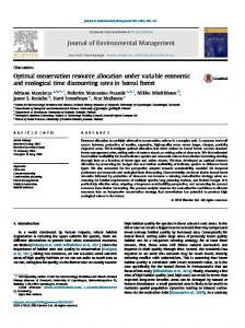
VII. R ESULTS A. Results for RQ1 (Validation and MOEA Comparison) The first part of RQ1 establishes if the proposed strategy is worth with respect to a random search. The random search model just picks up solutions that satisfy the constraints, by a pseudorandom number generator, as implemented by the jMetal framework. With all 4 MOEAs the random search has been statistically worse than any MOEA algorithm for both quality indicators10 , with a confidence greater than 99%. We do no longer consider it in the next research questions. RQ1.2 is about MOEAs comparison. Figure 2 shows the notched box plots for both indicators (IGD and Spread). The Friedman test yielded a p-value = 3.42 E-6 for IGD and pvalue = 1.08 E-6 for spread, rejecting the null hypothesis that all the MEOAs are statistically equivalent, for both indicators. Table IV reports the results of the Nemenyi test.

(a) IGD

(b) SPREAD

Fig. 2: Boxplots of the quality indicator TABLE IV: Comparison (P: PAES; N:NSGA-II; M: MOCELL; I: IBEA). Each cell contains a p-value (bold values indicate that the difference is ˆ1,2 (row, column) effect size measurement (for significant at  0.05) and a A ˆP,N = 0.785 both IGD and spread, the smaller the better – e.g., for IGD, A means P is bigger than N in terms of IGD, so it is worse). (a) IGD Indicator

(b) SPREAD Indicator

Pairwise Comparison: p-values N M I P .005/.78 .749/.61 .228/.36 I

Multi-Objective Testing Resource Allocation under Uncertainty - Unina

Multi-Objective Testing Resource Allocation under Uncertainty - Unina

Suggest Documents

Resource allocation under complete uncertainty

Resource allocation under channel uncertainty - EE@IITM

Distributed learning for resource allocation under uncertainty - mescal

Distributed learning for resource allocation under uncertainty - Mescal

International Portfolio Allocation under Model Uncertainty

ON OPTIMAL ALLOCATION OF INDlVlSlBLES UNDER UNCERTAINTY

Optimization models for resource allocation under ...

Efficient Resource Allocation under Acceptant ... - Google Sites

Resource-Bounded Scheduling Under Uncertainty - Semantic Scholar

Heterogeneous Resource Allocation under Degree ... - HAL-Inria

Plan Execution under Resource Consumption Uncertainty - Computer

Resource Allocation Under Delay-Guarantee ... - ePrints Soton

Cooperative Precoding/Resource Allocation Games under Spectral ...

Optimal conservation resource allocation under ... - Semantic Scholar

Optimizing Testing-Resource Allocation Using Architecture-Based

Efficient Resource Allocation using a Multiobjective Utility Optimisation

Nondifferentiable multiobjective programming under

Resource Co Resource Co-allocation in allocation

The Ricardian rent and the allocation of land under uncertainty ...

Resource Allocation for Interweave and Underlay CRs under ...

Optimal Constrained Resource Allocation Strategies under Low ... - arXiv

Efficient Resource Allocation under Multi-unit Demand - Google Sites

Optimal Computational Resource Allocation for Control Task under ...

Energy allocation in a reef coral under varying resource ... - Core