Multi-objective Transportation Network Design: Accelerating Search ...

2014 IEEE Congress on Evolutionary Computation (CEC) July 6-11, 2014, Beijing, China

Multi-objective Transportation Network Design: Accelerating Search by Applying ε-NSGAII Ties Brands, Luc. J. J. Wismans, and Eric C. van Berkum authority tries to find the best sustainable network, where travelers try to find the best travel options for themselves Sustainability is generally defined by multiple indicators, so in this paper we adopt a multi-objective network optimization approach (see also [1]). This enables us to find a set of Pareto-optimal network solutions, providing insight into tradeoffs between the different objectives (see also [2]). Network design problems (NDPs) have received a lot of attention in the literature, in many different versions. One subclass of problems is the transit network design problem, which has been studied in various ways [3]. Another subclass of problems is the unimodal road network design problem, which has also been studied in various ways [4]. Applications in a multimodal context are less common, but they do exists, for example road link capacity and bus routes [5] or pricing of private and public links [6]. The NDP is considered to be a multi-objective optimization problem in only a limited number of cases (for example [7-10]). To our knowledge, [5] is the only paper where multi-objective optimization and a multimodal NDP are combined. In their work, decision variables include both new street construction and lane additions / allocations as well as redesign of bus routes. Their focus was on the development of a metaheuristic to solve the bi-level problem. In fact they compared the performance of a hybrid genetic algorithm and a hybrid clonal selection algorithm for multiple test networks. In a number of papers metaheuristics were applied for solving the transit network design problem. For example [11-13] used a genetic algorithm and [14] used simulated annealing. [15] tested both scatter search and a genetic algorithm and [16] used a metaheuristic called GRASP (Greedy Randomized Adaptive Search Procedure). Previously, the evolutionary algorithm NSGAII [17] was used in a similar network optimization study, with focus on how the choice for random seeds influences the performance of NSGAII [18]. It appeared that specifically for the lower level, computation times were considerable. In addition to that, in this paper the case study is extended, leading to doubling of the calculation time needed for one function evaluation. This extension is desired, since a more detailed modelling of the underlying design problem leads to a more accurate calculation of objective function values. Therefore, in this paper we concentrate on the performance of an adaption of the NSGAII approach called ε-NSGAII that requires less solutions to be evaluated, and thus may improve computation times [19]. For this we applied both ε-NSGAII and the traditional NSGAII for a real life design case of a multimodal network in the metropolitan region of Amsterdam in the Netherlands.

Abstract— The optimization of infrastructure planning in a multimodal passenger transportation network is formulated as a multi-objective network design problem, with accessibility, use of urban space by parking, operating deficit and climate impact as objectives. Decision variables are the location of park and ride facilities, train stations and the frequency of public transport lines. For a real life case study the Pareto set is estimated by the Epsilon Non-dominated Sorting Genetic Algorithm (ε-NSGAII), since due to high computation time a high performance within a limited number of evaluated solutions is desired. As a benchmark, the NSGAII is used. In this paper Pareto sets from runs of both algorithms are analyzed and compared. The results show that after a reasonable computation time, ε-NSGAII outperforms NSGAII for the most important indicators, especially in the early stages of algorithm executions.

I. INTRODUCTION

H

IGHLY urbanized regions in the world nowadays face well-known sustainability problems in transport systems, like congestion, use of scarce space in cities by vehicles and the emission of greenhouse gases. A shift from car to public transport (PT) modes can alleviate these problems. Better utilization of the existing PT infrastructure without the need for large investments in new infrastructure may be achieved by facilitating an easy transfer from private modes (bicycle and car) to PT modes (bus, tram, metro and train). This can be done by network developments that enable multimodal trips, like opening new Park and Ride (P&R) facilities, opening new train stations or changing existing or opening new PT service lines. When we want to determine which investments can best be done, we also have to take into account the way in which travelers may alter their travel behavior, as a result of changes in the network. As a result our approach is a bi-level optimization problem, where in the upper level the network

T. Brands is PhD candidate at the Centre for Transport Studies of the University of Twente, Enschede, The Netherlands and consultant at Goudappel Coffeng, Deventer, The Netherlands (corresponding author) phone: 0031-53-4894704; fax: 0031-53-4894040; e-mail: [email protected]). L.J.J Wismans is senior consultant at DAT.Mobility (part of Goudappel Groep), Deventer, The Netherlands and associate professor at the Centre for Transport Studies of the University of Twente, Enschede, The Netherlands (e-mail: [email protected]). E.C. van Berkum is professor and head of the Centre for Transport Studies of the University of Twente, Enschede, The Netherlands (e-mail: [email protected]). This work was supported by The Netherlands Organisation for Scientific Research (NWO), in the program Sustainable Accessibility of the Randstad (SAR). This research is part of the project Strategy towards Sustainable and Reliable Multimodal Transport in the Randstad (SRMT). 978-1-4799-1488-3/14/$31.00 ©2014 IEEE

405

The remainder of this paper is organized as follows. Section 2 first mathematically defines the problem and describes the algorithms used to solve it. Section 2 also describes the practical case study that was solved in this paper. Section 3 presents the results of both algorithms applied to the case study, using various performance indicators. Finally, section 4 contains the conclusions and suggestions for further research.

characteristics Cu . All together, the transportation network is defined by G ( N , A, L,U ) , where A, L and U are further specified by Ca , Cl and Cu .

C. Optimization problem

We define a decision vector y (or a solution), that consists

II. PROBLEM DEFINITION

G N A L U R,S Ca Al Cl Cu M K rs Kˆ mrs f krs , fˆkmrs xa , x xˆal , xˆ

A. Bi-level problem We formulate the transportation network design problem as a bi-level optimization problem, since we want to incorporate the behavioral response of travelers to network changes, as was argued by [20-22]. The upper level represents the decision making of the transport network authority, which is reflected by the optimization of multiple system objectives, such as total travel time or the emission of greenhouse gases. In the lower level we assume that travelers try to find the best travel options for themselves, which is reflected by the maximization of their own utility which is usually based on several attributes such as travel time or travel cost. In this study we consider two main decision processes, i.e. route choice and mode choice, where also the choice for a combination of different modes is considered to be feasible. For this lower level, we assume a generalization of the traditional stochastic user equilibrium (e.g. see [23]) as the situation in which no driver believes he or she can improve his/her utility by unilaterally changing route or mode. Every network configuration that is considered in the upper level is input for the lower level. The equilibrium situation that is determined in the lower level now yields all the necessary input to determine the values of the multiple objective functions. So the bi-level approach regards this problem as a network optimization problem where the lower level is a constraint.

δ ars, k δˆalrs, km δ ars, km

t a ( xa , y ) tˆal ( y ) rs ckrs , cˆkm rs cˆm uˆ rs

rs ζ km

ψ mrs qrs , qrs qˆ rs , qˆ θ1 ,θ 2 ,θ 3

B. Definition of network and demand

Nj

Optimization problem and results Decision vector Set of feasible decision vectors Length of decision vector y Objective vector upper level Objective function lower level Length of objective vector Z . Number of optimization processes Set of solutions calculated during optimization process j Pareto set from optimization process j: all non-dominated j solutions in φ Number of solutions in Pareto set j

νa νp H πh φh ϑh σh ϕ I Ei

Genetic parameters Archive size Population size Number of generations (index h) Set of archive solutions in generation h Set of offspring solutions in generation h Union of archive and offspring in generation h Set of solutions in mating pool in generation h Mutation rate Number of restarts Size of ε-archive at restart i

y Y V Z z W J φj Pj

The multimodal transportation network is defined as a directed graph G, consisting of node set N, link set A, a line set L and a stop set U (see Table 1). For each link a one or more modes are defined that can traverse that link with a certain speed and capacity: the link characteristics Ca . Origins r ∈ R and destinations s ∈ S are a subset of N. Total fixed transportation demand qrs is stored in a matrix with size |R|×|S|, that contains trips from origin to destination (OD). Furthermore, transit service lines l ∈ L are defined as ordered subsets Al within A and can be stop services or express services. PT flows can only traverse transit service lines. Transit stations or stops u ∈ U are defined as a subset within N. Consequently, a line l traverses several stops. The travel time between two stops and the frequency of a transit service line l are stored as line characteristics Cl . Access / egress modes and PT are only connected through these stops. A combination of using a specific access mode, PT and a specific egress mode, is defined as a mode chain M. Whether a line calls at a stop u or not, is indicated by stop

406

TABLE 1 NOTATION Transportation network and demand Multimodal transportation network Node set N Link set A Line set L Stop set U Origin set, destination set Characteristics of link a Subset of links that is traversed by line l Characteristics of line l Characteristics of stop u Set of mode chains Set of car routes for OD pair r,s set of PT routes for OD pair r,s on mode chain m Route flow for car, route flow for PT mode chains Vehicle link flow, vehicle flow vector Passenger link flow per transit line, passenger flow vector Car route, vehicle link flow indicator PT route, passenger link and line indicator PT route, vehicle link indicator Cost function for car links Cost function for PT links per transit line Route costs for car, route costs for PT Combined costs for PT mode chains Combined costs for PT Fraction of travelers on OD pair r,s in PT mode chain m, choosing route k Fraction of PT travelers on OD pair r,s choosing mode chain m Total OD demand, car OD demand PT OD demand (from r to s), PT OD demand vector Logit parameters for mode choice, PT mode chain choice, PT route choice

of V discrete decision variables: y = { y1 ," , yv ," , yV } . Y is the set of feasible values for the decision vector y (also called decision space). The objective vector Z (consisting of W objective functions, Z = {Z1 ," , Z w ," , ZW } ) depends on the value of the decision vector y . Every Z is part of the so called objective space, and in principle Z may be any value in \W , but depending on its meaning, an objective function may be subject to natural bounds. The resulting multi-objective optimization problem (MOOP) is defined in (1-15). The lower level program in (3-15) is based on the formulation in [23]. The characteristics Ca , Cl and Cu of A, L and U depend on the decision vector y . These characteristics define the multimodal transportation network G. Feasibility constraint (2) should be satisfied to define a transportation network that is physically within reach. Constraint (3) represents the lower level optimization problem, that optimizes modal split and flows in the network from the travelers perspective and has equations (4-15) as constraints. The modal split model is a nested logit model [24], defined in formulas (3) and (12). Constraint (4) ensures that the sum of car route flows and PT demand are equal to the total demand qrs , where multimodal trips are included in PT demand: we see such trips as PT trips with various access and egress modes. Constraint (5) is a non-negativity constraint for car route flows. Note that PT route flows are nonnegative by the definitions in constraints (6-7). (6) ensures positive PT demand. (7) distributes PT demand over various mode chains and PT routes, using the fractions in constraints (12-13): (13) defines the route fractions for PT trips per mode chain: the PT model contains multiple routing, where trips are distributed among sensible routes using a logit model. Constraint (12) defines the mode chain fractions for PT trips. Constraint (10) calculates the OD based generalized costs per mode chain as a weighted average of route costs, to correctly take into account combined waiting costs of multiple transit lines. Constraint (9) calculates the logsum (the combined costs of all mode chains) to represent OD based PT costs. Constraints (8) and (11) define the relation between link costs and route costs, for car and for PT. The link costs ta ( xa , y ) and tˆal ( y ) depend on y through the link and line characteristics Ca and Cl . Finally, constraints (14-15) define the vehicle and passenger link flows based on car and PT route flows. Note that PT routes may contain car links, in the case of the use of a P&R facility in the route (see constraint 14). On the other hand, car routes never include PT passenger links, as can be observed in constraint (8).

min Z ( y, x, xˆ ) , s.t. y ∈Y

⎛1

∑ ∫ t (ω , y )dω + ∑ ∫ ⎜ θ ⎝ a

a∈ A 0

r ∈R , s∈S 0

1

ln

ω qrs − ω

⎞

+ uˆrs ⎟ d ω

f krs ≥ 0

∀r , s, k ∈ Kˆ mrs

(5)

qˆrs ≥ 0

∀r , s

(6)

∀r , s, m, k ∈ Kˆ mrs (7)

ckrs = ∑ ta ( xa , y )δ ars, k a∈ A

uˆrs = −

cˆmrs =

1

θ2

ln

∑ e−θ cˆ

rs 2 m

∀r , s, k ∈ Kˆ mrs

(8)

∀r , s

(9)

∀r , s, m

(10)

m∈M

∑ ζ kmrs cˆkmrs

k∈Kˆ mrs

⎛ ⎞ rs = ∑ ⎜ ta ( xa , y )δ ars, km + ∑ tˆal ( y )δˆalrs, km ⎟ cˆkm ⎠ a∈ A ⎝ l∈L

∀r , s, m, k ∈ Kˆ mrs (11) rs

ψ mrs =

e −θ2 cˆm

∀r , s, m

∑ e−θ cˆ

rs 2 m

(12)

m∈M

rs

rs ζ km =

e −θ3cˆkm

∑

∀r , s, m, k ∈ Kˆ mrs (13)

rs

e −θ3cˆkm

k ∈Kˆ mrs

xa = ∑∑

∑

r∈R s∈S k ∈{ Kˆ rs }

xˆal = ∑ ∑

f krsδ ars, k + ∑∑ ∑

∑ ∑

r∈R s∈S m∈M k ∈{ Kˆ mrs }

r∈R s∈S m∈M

fˆkmrsδˆalrs, km

∑

k ∈{ Kˆ mrs }

fˆkmrsδ ars, km

∀a

(14)

∀a, l

(15)

D. Solution methods The MOOP defined in (1-15) is an NP-hard problem, since the bi-level linear programming problem is already an NP-hard problem [25]. Therefore, the problem is computationally too expensive to be solved exactly for larger networks, so we rely on a heuristic. For solving multi-objective problems, the class of genetic algorithms is often used, because these algorithms have a low risk of ending up in a local minimum, do not require the calculation of a gradient and are able to produce a diverse Pareto set [26]. More specifically, we use algorithms NSGAII and ε-NSGAII developed in respectively [27] and [19]. Both algorithms optimize multiple objectives simultaneously, searching for a set of non-dominated solutions, i.e. the Pareto set. NSGAII has been successfully applied by researchers to solve multi-objective optimization problems in traffic engineering and proved to be efficient for this type of problems with respect to other types of genetic algorithms [1, 28]. For ε-NSGAII, [19] found that on their test problems ε-NSGAII appeared to perform better than NSGAII in terms of attained hypervolume and distance to the real Pareto set, especially in the early stage of the algorithm. Especially this

x, xˆ , qˆ = arg min z ( x, xˆ , qˆ ) = qˆ rs

(4)

rs fˆkmrs = ψ mrsζ km qˆrs

(2)

xa

f krs + qˆrs = qrs

k ∈K rs

(1)

y

∑

∀r , s

s.t.

(3)

⎠

407

good performance in limited number of iterations is very beneficial for computationally highly expensive problems, like our optimization problem. In this paper we test the performance of both algorithms on a real world optimization problem with expensive objective function calculation. This generates additional insights in the performance of especially ε-NSGAII, since literature only provides limited evidence of the operational performance of ε-NSGAII.

Step 6: Variation: Apply recombination (uniform crossover) and mutation operators to the mating pool σ g +1 to create offspring φh +1 . Set h = h + 1 and go to step 2.

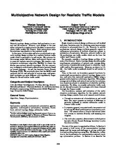
2) ε-NSGAII ε-NSGAII has NSGAII as a basis, but adds two main elements: ε-dominance and restarts with adaptive population sizing (see Fig. 1).

1) NSGAII Within NSGAII, the mating selection is done by binary tournament selection with replacement. In addition to this mating process, a random mutation operator is applied to a (small) fraction ϕ of solutions from each generation, to promote the exploration of unexplored regions in the decision space. These aspects of the algorithm make that the result is an approximation of the true Pareto set. In case an infeasible solution is generated during either recombination or mutation, that solution is discarded and a new solution is generated by repeating the recombination or mutation operator until a feasible solution is generated. The fitness value is calculated in two steps. In the first step (non-dominated sorting), the solutions are ranked based on Pareto dominance. All solutions in the Pareto set receive rank 1. In the next step, these solutions are extracted from the set and all Pareto solutions in the remaining set receive rank 2, etc. In the second step, the solutions are sorted within these ranks based on their crowding distance. Crowding distance calculation requires sorting of the population according to each objective value. The extreme values for each objective are assigned an infinite value, assuring that these values survive. All intermediate solutions are assigned a value equal to the difference in the normalized function values of two adjacent solutions. Concluding, the crowding distance value (and thus the fitness value) is higher if a solution is more isolated, promoting a more diverse Pareto set. The algorithm in steps (for more details, the reader is referred to [17]): Step 1: Initialization: Set population size ν p , which is equal to the archive size ν a , the maximum number of generations H, and generate an initial population φ0 . Set h = 0 and π 0 = ∅ . Step 2: Fitness assignment: Combine archive π h and offspring φh , forming ϑh = π h ∪ φh and calculate fitness values of solutions by dominance ranking and crowded distance sorting. Step 3: Environmental selection: Determine new archive π h +1 by selecting the ν a best solutions out of ϑh based on their fitness. Step 4: Termination: If h ≥ H or another stopping criteria is satisfied, determine Pareto set P from the set of all calculated solutions φ = {φ0 ∪ " ∪ φH } (non-dominated solutions). Step 5: Mating selection: Perform binary tournament selection with replacement on π h +1 to determine the mating pool of parents σ h +1 .

Initial population

NSGA-II until convergence

ε-archive of size Ei 2Ei newly generated random solutions

After fixed number of restarts I: STOP

Starting population for next restart

Fig. 1. The main loop of the ε-NSGAII algorithm

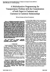
For every objective, an ε-value has to be set, resulting in an ε-grid in the objective space. In this way, every Pareto solution is placed within one ε-box (see Fig. 2). This allows the user to specify the precision of the algorithm for each objective. The concept of ε-dominance is defined as follows. As a first step, only one Pareto solution is chosen to represent an ε-box. If that box contains more than one Pareto solution, the solution that is closest to the vertex of the hyperbox with minimum objective value for all objectives is chosen. When determining this distance, the Euclidian distance is calculated, using the specified ε-values to normalize the objective values. As a second step, boxes that are dominated by another box (i.e., have a worse or equal objective value for every objective) are eliminated. The objective value for a box is chosen to be the minimum value of all objectives in the box (similar to the vertex of the hyperbox used to find the best Pareto solution per ε-box in step 1). The solutions that are contained by every remaining ε-box are denoted as the ε-Pareto set. During every generation of the NSGAII algorithm, in which the Pareto set is determined by non-domination sorting, the ε-Pareto set is also determined and saved in an ε-archive. This ε-archive is updated every generation by applying ε-dominance over the union of the archive of generation h-1 and the Pareto set of generation h. When no progress is made any more in the ε-archive for a specified number of generations, a restart is activated, where the starting population after the restart consists of the ε-archive, replenished with new randomly generated solutions. The generation size after the restart depends on the size of the ε-archive: the larger the archive, the larger the generation size. The setting of ε is very important, since it determines the tradeoff between precision and speed of the algorithm.

408

Objective 1

- Frequencies of 8 major bus lines, that can take 4 different discrete values - Opening or closing of 7 park-and-ride facilities (binary variable) - Opening or closing of 6 train stations (binary variable) - Marking 3 train stations as express station or not (binary variable). All decision variables are denoted as yv and are contained in vector y . Binary variables are directly represented in the genetic string. Variables that can take 4 different values are represented by 2 genes in the genetic string. In total, decision space Y contains approximately 7E+10 different values for the decision vector y .

ε2

ε1 Objective 2

Objective 1

2) Objective functions In this paper we consider 4 objectives which we want to minimize: total travel time in the whole network, urban space used by parking, operating deficit of the public transport system and climate impact of the transport system. The values of the objective functions are calculated as follows based on loads and travel times in the network G ( N , A, L,U ) and on demand matrices after applying the lower level. Total travel time involves travel time of car users and PT users. Urban space used by parking follows from demand matrices for car and Park and Ride. Operating deficit is the difference between operating costs and operating revenues, that depend on PT ridership. Finally, CO2 emissions are calculated from network loads using emission factors. More details on objective function calculation can be found in [18].

Objective 2

Fig. 2. Illustration of ε-dominance for the 2 objective case. Top: step 1, choosing 1 solution per ε-box. Bottom: step 2, applying dominance to the ε-boxes: the light grey boxes are dominated by the darker boxes.

E. Case study The case study area covers the Amsterdam Metropolitan Area in The Netherlands (Fig. 3). This region is characterized by dense concentrations of housing, employment and facilities, high costs for parking in city centers due to the scarcity of space, and congested road networks. Origins and destinations are aggregated into 102 transportation zones. Important commercial areas are the city centers of Amsterdam and Haarlem, the business district in the southern part of Amsterdam, the harbor area and airport Schiphol. Other areas are mainly residential, but still small or medium scale commercial activities can be found. We assume a fixed demand for transportation that is based on the mentioned socio-economic characteristics of the area and is taken from the regional transportation model (named Venom), that is used for planning by the authorities [29]. Travelers are served by an extensive multimodal network with pedestrian, bicycle, car and transit infrastructure. Transit consists of bus, tram, light rail, bus rapid transit, metro, local train, regional train and intercity train. Bicycles can be parked at most stops and stations, and 36 transit stations facilitate park-and-ride transfers.

Zaanstad

Almere

Haarlem Amsterdam

Hoofddorp

Schiphol

Fig. 3. The study area of the case study, containing various urban areas, roads, railroads, train lines and bus lines.

3) Parameter settings To limit computation time, in this study we set the maximum number of evaluated solutions at 2640. For each of these solutions 4 objective function values are calculated. In that case the computation time is just under two weeks, since the evaluation of one solution takes approximately 6.5 minutes (using a computer with an Intel® Core™ i7 CPU 860

1) Decision variables At various locations in this transportation network, 36 decision variables are defined: - Frequencies of 12 train lines, that can take 2 or 4 different discrete values 409

A. Minimum per objective In Fig. 4 we show the normalized values of the objective function that are achieved per run (the value of the objective function of NSGAII, run 1 is rescaled to 100). For all objectives except total travel time ε-NSGAII outperforms NSGAII, but differences are small. For total travel time however ε-NSGAII performs considerably worse than NSGAII for run 1. For run 2 differences are very small. Index (NSGA-II run 1 equals 100)

@ 2.8GHz and a 4 GB RAM). For NSGAII, we used a generation size of 80, resulting in 33 generations to come to 2640 evaluated solutions. For ε-NSGAII, the parameters from [19] could not be used (the computation time would be too large), so we used a test problem to come to appropriate settings. This test problem is comparable with our real life problem (equal number of objectives and equal decision space), but had small computation times. This resulted in the following settings that yielded approximately the desired number of function evaluations. A 1/3 injection scheme was used, implying that at every restart, 1/3 of the new starting population will consist of the ε-archive and 2/3 of new randomly generated solutions. Next, the parameter for convergence that triggers a restart was set such that after 3 generations without a change in the ε-archive, a restart is activated. The number of restarts is set as 5 and the initial population size is set as 10. Finally, the ε values are set per objective. The range that is known for each objective bounded by the minimum and maximum known values is divided into 5 to 8 ε-boxes. This results in approximately 2000 boxes in the objective space. However, since the Pareto set contains a certain structure by definition (i.e. in the 2-dimensional case the Pareto set is a line and in the multidimensional case a hyperplane), a majority of the boxes is empty. Step 2 (see Fig. 2) further reduces the ε-Pareto set, resulting in a typical size of approximately 25 solutions in the application in this paper.

110 108 106 104 102 100 98 96 94 92 90

NSGA-II, run 1 NSGA-II, run 2 ε-NSGAII, run 1 ε-NSGAII, run 2

Total Urban Operating CO2 travel time space used costs emissions

Fig. 4. The normalized values found by the 4 runs.

B. Hypervolume The next indicator that is considered is the hypervolume indicator [30], also known as S-metric or space coverage. In the 2-dimensional case it determines the area that is covered by the Pareto set with respect to a reference point, i.e. the upper bound of all objectives. This is defined such that it is dominated by all solutions in the Pareto set. Because the true maximum values of the objective functions are not known, a

III. RESULTS In this section we show the results of 4 optimization runs: 2 using NSGAII and 2 using ε-NSGAII. Both runs of the same algorithm differ, because both algorithms use a random seed in Monte Carlo simulation that is used for the recombination and mutation operators in the genetic algorithm. [18] elaborate more on these differences due to random seeds. To assess the differences, well known indicators from the literature are used in the coming sections. With the chosen parameter settings for ε-NSGAII, run 1 results in 2631 calculated solutions and run 2 in 2330 calculated solutions. This difference occurred because the stop criterion is met at a different moment in time for the two runs with different random seeds. For NSGAII, 2640 solutions are calculated to have a (fixed) calculation time that is comparable, but never shorter than the calculation time of ε-NSGAII. Since we would like to use all available information concerning objective function values (that were gathered in the lower level by expensive calculations in terms of calculation time), we use all calculated solutions within one run to determine the Pareto set for that run. An alternative would be to analyze the Pareto set resulting from the final generation of the genetic algorithm. As said, we do not choose to do this, because the generation size (and thus size of the Pareto set) in NSGAII and ε-NSGAII have a considerably different size. Further, the calculation of the Pareto set from a few thousand solutions, and calculation of the values of the performance indicators is possible in reasonable calculation time, making it feasible to use all known objective function values to determine the Pareto set and the indicator values.

TABLE 2 THE NORMALIZED HYPERVOLUME VALUES FOR FOUR OPTIMIZATION RUNS

NSGAII, run 1 NSGAII, run 2 ε-NSGAII, run 1 ε-NSGAII, run 2

Number of Pareto solutions N j 173 192 203 229

Normalized hypervolume 0.990 0.985 0.999 1.000

conservative point is chosen. In the multi-dimensional case this area becomes a so-called hypervolume. Since we formulated the problem as a minimization problem for all objectives, a larger hypervolume means a better solution. In Table 2 we show the normalized hypervolume values for the Pareto sets resulting from the 4 optimization runs. For both runs ε-NSGAII outperforms NSGAII. Note that ε-NSGAII has more solutions in the final Pareto sets, which is one reason for this better performance.

1) Convergence In Fig. 5 we show the hypervolume as a function of the number of evaluated solutions until that moment in time. The hypervolume is calculated based on the Pareto set that is known with respect to all solutions calculated until that moment in time. In Fig. 6 we plotted the size of the corresponding Pareto sets. Note that the hypervolume value never decreases, since each new solution either improves the Pareto set or the Pareto set remains the same. We observe that ε-NSGAII converges very fast in terms of hypervolume.

410

Results show that we can stop the iterative procedure after 2000 solutions.

TABLE 3 COVERAGE OF THE RUN IN THE ROW OVER THE RUN IN THE COLUMN NSGAII ε-NSGAII run 1 run 2 run 1 run 2 NSGAII, run 1 0.36 0.24 0.21 NSGAII, run 2 0.31 0.21 0.26 ε-NSGAII, run 1 0.49 0.43 0.28 ε-NSGAII, run 2 0.50 0.48 0.30

Relative hypervolume covered

1.00 0.98 0.96 0.94 0.92

D. Algorithm comparison Putting these results together, ε-NSGAII shows better results for the experiments in this paper than NSGAII with respect to set coverage and hypervolume. Furthermore, for the best solutions for each individual objective ε-NSGAII scored better for 3 out of 4 objectives, but the objective travel time showed considerably worse values. The high performance of ε-NSGAII may be explained by the focus on large gains by the ε-dominance relation: if no large progress is made any more, no computation time is wasted to achieve little improvement. Instead, a restart is triggered, stimulating exploration of new areas of the front, but using the properties of the high quality solutions found earlier (the ε-archive). Another explanation may be the dynamic population size: by starting with a small population, the algorithm focusses on dominance rather than on producing a diverse Pareto set. In limited calculation time large progress is made in an early stage of the algorithm. Later, the population size grows, allowing for more diverse solutions, but is directly dependent on the size of the ε-archive, so that no calculation time is wasted on too much detail. The results imply that for finding the extreme solutions, ε-NSGAII seems less suitable. However, the main reason for applying multi-objective optimization is to find good tradeoff solutions and not to find the minimum values of individual objectives (otherwise single objective optimization would be sufficient).

0.90 0.88 0.86 0.84 0.82

2700

2500

2300

2100

1900

1700

1500

1300

900

1100

700

500

300

100

0.80

Number of evaluated solutions NSGA-II, run 1

NSGA-II, run 2

ε-NSGAII, run 1

ε-NSGAII, run 2

Fig. 5. The hypervolume covered with respect to the number of evaluated solutions.

Number of Pareto solutions found

250

200

150

100

50

2700

2500

2300

2100

1900

1700

1500

1300

1100

900

700

500

300

100

0

Number of evaluated solutions NSGA-II, run 1

NSGA-II, run 2

ε-NSGAII, run 1

ε-NSGAII, run 2

IV. CONCLUSION In this paper, we formulated the multimodal passenger transportation network design problem as a multi-objective optimization problem, to minimize total travel time, use of urban space by parking, operating deficit and climate impact. Considering the high computation times in our real life case study, we need a solution method that uses a limited number of evaluated solutions. Therefore, this paper compares the performance of the multi-objective algorithms NSGAII and ε-NSGAII when applied to our multimodal network design problem. The case study in this paper confirms earlier findings that ε-NSGAII outperforms NSGAII on most indicators [19]. Especially in the early stages of the algorithm execution, large progress is observed. On the other hand, ε-NSGAII did not find better values for all individual objective functions. From this, we can conclude that ε-NSGAII is an efficient algorithm to find high quality tradeoff solutions in our multi-objective optimization problem, especially because objective function calculation is highly computationally expensive. It performs comparable with NSGAII to find the

Fig. 6. The size of the found Pareto set with respect to the number of evaluated solutions

C. Set coverage Finally the Pareto sets are compared using the set coverage indicator or C-metric [31]. The set coverage is a pairwise indicator that shows the fraction of solutions in the other set that is dominated by solutions in a set. This definition implies that a higher value for a Pareto set indicates a better score over the set that it is compared with. In Table 3 we show the values for set coverage for all pairs to be formed out of the 4 optimization runs. It can be seen that comparing ε-NSGAII with NSGAII Pareto sets results in considerable higher values than the other way around. Note that the set coverage of run 1 and run 2 with the same algorithm shows the influence of the random seeds: the set coverage reveals that both runs are not completely symmetrical: although the difference between the values is not very high.

411

extreme ends of the Pareto set. For future research it would be interesting to investigate the influence of different settings of ε on the results. ε-settings can be used to put emphasis on specific objectives, but also strongly influence calculation times, since convergence of the algorithm depends on them. Furthermore, since results of evolutionary algorithms are always case specific, it would be good to do more similar tests on different real life design problems.

[15]

[16] [17] [18]

ACKNOWLEDGMENT The authors thank the City Region of Amsterdam for the use of the data from the regional transport model Venom.

[19]

REFERENCES [1]

[2]

[3] [4] [5]

[6]

[7] [8]

[9] [10]

[11]

[12] [13]

[14]

L. J. J. Wismans, E. C. van Berkum, and M. C. J. Bliemer, "Comparison of Multiobjective Evolutionary Algorithms for Optimization of Externalities by Using Dynamic Traffic Management Measures," Transportation Research Record: Journal of the Transportation Research Board, vol. 2263, pp. 163-173, 2011. C. Coello, S. de Computación, and C. Zacatenco, "Twenty years of evolutionary multi-objective optimization: A historical view of the field," IEEE Computational Intelligence Magazine, vol. 1, pp. 28-36, 2006. V. Guihaire and J. K. Hao, "Transit network design and scheduling: A global review," Transportation Research Part A: Policy and Practice, vol. 42, pp. 1251-1273, 2008. H. Yang and M. Bell, "Models and algorithms for road network design: a review and some new developments," Transport Reviews, vol. 18, pp. 257-278, 1998. E. Miandoabchi, R. Farahani, W. Dullaert, and W. Szeto, "Hybrid Evolutionary Metaheuristics for Concurrent Multi-Objective Design of Urban Road and Public Transit Networks," Networks and Spatial Economics, vol. 12, pp. 441-480, 2012. Y. Hamdouch, M. Florian, D. Hearn, and S. Lawphongpanich, "Congestion pricing for multi-modal transportation systems," Transportation Research Part B: Methodological, vol. 41, pp. 275-291, 2007. A. Sumalee, S. Shepherd, and A. May, "Road user charging design: dealing with multi-objectives and constraints," Transportation, vol. 36, pp. 167-186, 2009. L. J. J. Wismans, E. C. Van Berkum, and M. C. J. Bliemer, "Comparison of Multiobjective Evolutionary Algorithms for Optimization of Externalities by Using Dynamic Traffic Management Measures," Transportation Research Record: Journal of the Transportation Research Board, vol. 2263, pp. 163-173, 2011. A. Chen, J. Kim, S. Lee, and Y. Kim, "Stochastic multi-objective models for network design problem," Expert Systems with Applications, vol. 37, pp. 1608-1619, 2010. S. Sharma, S. Ukkusuri, and T. Mathew, "Pareto Optimal Multiobjective Optimization for Robust Transportation Network Design Problem," Transportation Research Record: Journal of the Transportation Research Board, vol. 2090, pp. 95-104, 2009. B. Beltran, S. Carrese, E. Cipriani, and M. Petrelli, "Transit network design with allocation of green vehicles: A genetic algorithm approach," Transportation Research Part C: Emerging Technologies, vol. 17, pp. 475-483, 2009. P. Chakroborty, "Genetic Algorithms for Optimal Urban Transit Network Design," Computer-Aided Civil and Infrastructure Engineering, vol. 18, pp. 184-200, 2003. E. Cipriani, S. Gori, and M. Petrelli, "Transit network design: A procedure and an application to a large urban area," Transportation Research Part C: Emerging Technologies, vol. 20, pp. 3-14, 2012. W. Fan and R. Machemehl, "Optimal Transit Route Network Design Problem with Variable Transit Demand: Genetic Algorithm Approach," Journal of Transportation Engineering,

[20]

[21] [22]

[23] [24] [25] [26] [27]

[28]

[29] [30] [31]

412

vol. 132, pp. 40-51, 2006. M. Gallo, B. Montella, and L. D’Acierno, "The transit network design problem with elastic demand and internalisation of external costs: An application to rail frequency optimisation," Transportation Research Part C: Emerging Technologies, vol. 19, pp. 1276-1305, 2011. A. Mauttone and M. Urquhart, "A multi-objective metaheuristic approach for the transit network design problem," Public Transport, vol. 1, pp. 253-273, 2009. K. Deb, A. Pratap, S. Agarwal, and T. Meyarivan, "A fast and elitist multiobjective genetic algorithm: NSGA-II," Evolutionary Computation, IEEE Transactions on, vol. 6, pp. 182-197, 2002. T. Brands and E. C. van Berkum, "Performance of a genetic algorithm for solving the multi-objective, multimodal transportation network design problem.," International Journal of Transportation, vol. paper accepted for publication, 2014. J. B. Kollat and P. M. Reed, "Comparing state-of-the-art evolutionary multi-objective algorithms for long-term groundwater monitoring design," Advances in Water Resources, vol. 29, pp. 792-807, 2006. L. dell'Olio, J. Moura, and A. Ibeas, "Bi-Level Mathematical Programming Model for Locating Bus Stops and Optimizing Frequencies," Transportation Research Record: Journal of the Transportation Research Board, vol. 1971, pp. 23-31, 2006. S. Tahmasseby, "Reliability in urban public transport network assessment and design," T2009/6, TRAIL thesis series, TU Delft, Delft, 2009. F. Viti, S. F. Catalano, M. Li, C. Lindveld, and H. J. van Zuylen, "Optimization Problem with Dynamic Route-Departure Time Choice and Pricing," presented at the 82nd Annual Meeting of the Transportation Research Board, Washington, D.C., 2003. Y. Sheffi, Urban transportation networks: Equilibrium analysis with mathematical programming methods. Englewood Cliffs, New Jersey: Prentice-Hall, 1985. M. Ben-Akiva and M. Bierlaire, "Discrete choice methods and their applications to short term travel decisions," in Handbook of transportation science, ed: Springer, 1999, pp. 5-33. Z. Gao, J. Wu, and H. Sun, "Solution algorithm for the bi-level discrete network design problem," Transportation Research Part B: Methodological, vol. 39, pp. 479-495, 2005. K. Deb, Multi objective Optimization Using Evolutionary Algorithms. Chichester, UK: John Wiley & Sons, 2001. K. Deb, A. Pratap, S. Agarwal, and T. Meyarivan, "A fast and elitist multiobjective genetic algorithm: NSGA-II," IEEE transactions on evolutionary computation, vol. 6, pp. 182-197, 2002. S. Sharma, S. Ukkusuri, and T. Mathew, "Pareto Optimal Multiobjective Optimization for Robust Transportation Network Design Problem," Transportation Research Record: Journal of the Transportation Research Board, vol. 2090, pp. 95-104, 2009. S. Kieft, "Handboek Venom (in Dutch)," Stadsregio Amsterdam, The Netherlands, Versie 2.0, 17 October 2013. L. While, P. Hingston, L. Barone, and S. Huband, "A faster algorithm for calculating hypervolume," Evolutionary Computation, IEEE Transactions on, vol. 10, pp. 29-38, 2006. E. Zitzler and L. Thiele, "Multiobjective evolutionary algorithms: A comparative case study and the strength pareto approach," IEEE transactions on evolutionary computation, vol. 3, p. 257, 1999.