Please check the .m file for the Matlab implementation of the MPAV method. ..... [px,py] = gradient(imfilter(double(temp_wien),fspecial('Gaussian',[5 5],1),'same' ...
Multi-Pass Adaptive Voting for Nuclei Detection in Histopathological Images Supplementary information
Cheng Lu, Hongming Xu, Jun Xu, Hannah Gilmore, Mrinal Mandal, and Anant Madabhush
S1: Parameters Selection in Initial processing In the initial processing, there are two parameters involved, one with the Gaussian filter (denoted as 𝜎"#$ ) and the other with the Canny filter for edge detection (denoted as TCanny ). 𝜎"#$ is the width of the Gaussian filter, 𝜎"#$ is generally an odd integer for image smoothing. The higher the value of 𝜎"#$ , the smoother the output image. TCanny is the edge threshold used for Canny filtering. In Canny filtering, the gradient of the image is first computed. Based on the gradient magnitude map, TCanny maybe set to a high value for retaining all high gradient magnitude pixels, while TCanny x 0.4 (lower threshold) may be used to remove all the low gradient magnitude pixels. A connectivity check is performed to see if the pixels with intermediate gradient magnitude are connected to the high gradient magnitude pixels. The resulting pixels form the subsequent edge map. The value for TCanny is set relative to the highest value of the gradient magnitude within the image. We performed an experiment on evaluating 𝜎"#$ and TCanny with respect to the AUC. In the experiment, 𝜎"#$ Î [3,5,7,9,11,13], TCanny Î [0.45, 0.55,0.65,0.75,0.85], and the AUC is evaluated within Dataset A. AUC is a function of different parameters (𝜎"#$ and TCanny), shown in a 3D plot in Figure 1. One may observe that the performance is less affected by the Gaussian smoothing operation. The MPAV technique achieves max AUC when TCanny =0.65. And the AUC maintains high when TCanny is in the range of 0.55 to 0.75. The reason is that if TCanny is set to a small value, a large number of noisy pixels that do not belong to the nuclei edges are conflated which adversely affects the voting inference. On the other hand, increasing the value of TCanny will result in a decrease in the number of noisy pixels, potentially leading to better voting inferences being made. However, if TCanny is too high, very few pixels will be engaged in the voting process, in turn leading to lower voting accuracy (as shown in Figure 2). A detailed explanation of this Figure and the accompanying explanation are included in the supplementary material section. S2: Parameters Selection of Voting Area The size of the voting area is mainly controlled by two parameters rmax and Δ. rmax determines the voting range, that is, larger the rmax, the larger the corresponding voting area. For the task of nuclei detection, rmax can be set to a value close to the diameter of a typical nucleus. For example, for a tissue slide digitized at 40x magnification, rmax can be set to 40 pixels. Δ is a set of angular values, % % % e.g., we set Δ=( , , ). Each angular value in Δ will determine the size of fan-like voting area at & ( )*
each iteration. Smaller the angular value, smaller the voting area. Since the voting method uses the convergence/overlapping of voting area to infer the centroids of nuclei, the initial angular value cannot be set to a large value. For example, if the number of iterations N=3, then we set % % % Δ=( , , ), note that the number of iterations N is associated with each value in Δ. The initial & ( )*
%
angle is set to . As the number of iterations increase, the angular value decreases, and the size &
of the corresponding voting area decreases. This results in a narrower convergence region for voting with subsequent iterations. An illustration of VN. with different voting angles and at different iterations is shown in Figure 3. S3: Matlab implementation of the MPAV method. Please check the .m file for the Matlab implementation of the MPAV method.
1
0.8
0.95 0.9
AUC
0.85
0.75
0.8
0.75 0.7 0.65
0.7
0.6 0.55 0.5 13
0.65
11 9 7 5
100,IM,3,'MPAV-GRS2'); end function [Gx,Gy,IM_ws,bw,bw_CloseEdges]=LgenerateRetifiedGradientMap4Voting(IM,Para) T_PixelNOinComp=Para.T_PixelNuminComp; % control the edge fragment that go for voting Para.Method=Para.Preprocess_Method; [Gx,Gy,IM_ws,bw,bw_CloseEdges]=LpreprocessIM4MPV(IM,Para); px=Gx; py=Gy; % show(bw); cc=bwconncomp(bw); ss=regionprops(cc,'ConvexHull','PixelIdxList','Centroid'); for i=1:cc.NumObjects curPixelsList=ss(i).PixelIdxList; numPixels=length(curPixelsList); if numPixels>T_PixelNOinComp curHull=ss(i).ConvexHull; bw_curEdge=zeros(size(bw)); bw_curEdge(curPixelsList)=1;
bw_curHull=poly2mask(curHull(:,1),curHull(:,2),size(bw,1),size(bw,2)); cc_hull=bwconncomp(bw_curHull); ss_hull=regionprops(cc_hull,'Centroid'); curHullCentroid=ss_hull.Centroid; if Para.debug % show the graident info and centroid within the hull show(bw_curHull,14); hold on; pxshown=px; pyshown=py; pxshown(~bw_curEdge)=0;pyshown(~bw_curEdge)=0; quiver(-pxshown,-pyshown,5,'g'); plot(curHullCentroid(1),curHullCentroid(2),'rp','MarkerSize',20); hold off; show(bw_curEdge,15); hold on; pxshown=px; pyshown=py; pxshown(~bw_curEdge)=0;pyshown(~bw_curEdge)=0; quiver(-pxshown,-pyshown,5,'g'); hold off; end % for each pixel with valid gradient(i.e., G>0), we retify its gradient direction % debug version here AllBadG=[]; % record gradient locations AllGoodG=[]; for j=1:numPixels [curP_y,curP_x]=ind2sub(size(bw),curPixelsList(j)); if Para.debug % show(bw_curHull,14); hold on; % pxshown=px; pyshown=py;
% pxshown(~bw_curEdge)=0;pyshown(~bw_curEdge)=0; % quiver(-pxshown,-pyshown,5,'b'); % plot(curHullCentroid(1),curHullCentroid(2),'rp','MarkerSize',20); % plot(curP_x,curP_y,'rs'); % hold off; end curPG_x=px(curPixelsList(j));curPG_y=py(curPixelsList(j)); % vector_PC=curHullCentroid-[curP_x,curP_y]; % this one should % be correct,why? vector_PC=[curP_x,curP_y]-curHullCentroid; angle=acos(sum(vector_PC.*[curPG_x,curPG_y])/(norm(vector_PC)*norm([curPG_x,curPG_y]))); % pick gradient based on angle if ~(00 AllBadG_List=sub2ind(size(bw),AllBadG(:,2),AllBadG(:,1)); Gx(AllBadG_List)=-Gx(AllBadG_List); Gy(AllBadG_List)=-Gy(AllBadG_List); end end if Para.debug show(bw_curHull,17); hold on; pxshown=Gx; pyshown=Gy; pxshown(~bw_curEdge)=0;pyshown(~bw_curEdge)=0; quiver(-pxshown,-pyshown,5,'b');
plot(curHullCentroid(1),curHullCentroid(2),'ro','MarkerSize',20); if ~isempty(AllBadG) plot(AllBadG(:,1),AllBadG(:,2),'ks'); end if ~isempty(AllGoodG) plot(AllGoodG(:,1),AllGoodG(:,2),'rp','MarkerSize',10); hold off; end end end end end function [Gx,Gy,IM_ws,bw,bw_CloseEdges]=LpreprocessIM4MPV(IM,Para) if isempty(Para.Gaussian_sigma) Para.Gaussian_sigma=5; end %% M-------- GaussianSmooth_Hysthersh if strcmp(Para.Method,'GaussianSmooth_Hysthersh') % smooth image IM_ws=imfilter(double(IM),fspecial('Gaussian',[5 5],1),'same','conv','replicate'); [Gx,Gy] = gradient(IM_ws);% gradiet maps that will return % let the edges connecting bw = hysthresh(255-IM_ws, 70, 100); end %% M-------- GaussianSmooth_Hysthersh if strcmp(Para.Method,'GaussianSmooth_RemoveClosed') % smooth image
IM_ws=imfilter(double(IM),fspecial('Gaussian',[Para.Gaussian_sigma Para.Gaussian_sigma],1),'same','conv','replicate'); % show(IM_ws); [Gx,Gy] = gradient(IM_ws);% gradiet maps that will return %% for closed edges, we treat them as nuclei boundary and pick them out first % CannyEdgeThreshold=0.55;% higher, less edges CannyEdgeThreshold=Para.CannyEdgeThreshold; IM_edge=edge(IM_ws, 'canny',CannyEdgeThreshold); % show(IM_edge); IM_fill=imfill(IM_edge,'holes'); % show(IM_fill); IM_temp=IM_fill&~IM_edge; % show(IM_temp); IM_temp_d=imreconstruct(IM_temp,IM_fill); bw_CloseEdges=LgetValidNucleifromClosedEdges(IM_temp_d,0.65); % show(bw_CloseEdges); IM_edge_left= IM_edge&~bw_CloseEdges; % show(IM_edge_left) if Para.show LshowTwoKindofCountouronIM(bw_CloseEdges, IM_edge_left,IM_ws,6); end % bw=IM_edge_left; %% remove the long edge fragments, since they are definitely the noise fragments bw=LremoveHighAxisRatio(IM_edge_left,5); end %% M-------- if strcmp(Para.Method,'Wiener_RemoveNoise') %%
CannyEdgeThreshold=Para.CannyEdgeThreshold; Para_wiener=[4 4]; temp_wien = wiener2(IM,Para_wiener); % show(temp_wien,2) IM_ws=temp_wien; temp_edge=edge(temp_wien, 'canny',CannyEdgeThreshold); % [px,py] = gradient(imfilter(double(temp_wien),fspecial('Gaussian',[5 5],1),'same','conv','replicate')); [px,py] = gradient(double(temp_wien)); bw_edge=temp_edge; px(~bw_edge)=0;py(~bw_edge)=0; if Para.show show(bw_edge,53);hold on; quiver(-px,-py,5,'b'); hold off; end %% for closed edges, we treat them as nuclei boundary and pick them out first temp_wien = wiener2(IM,Para_wiener); % show(temp_wien,2) IM_edge=edge(temp_wien, 'canny',CannyEdgeThreshold); IM_fill=imfill(IM_edge,'holes'); % show(IM_fill); IM_temp=IM_fill&~IM_edge; % show(IM_temp); IM_temp_d=imreconstruct(IM_temp,IM_fill);
bw_CloseEdges=LgetValidNucleifromClosedEdges(IM_temp_d,0.65); IM_edge_left= IM_edge&~bw_CloseEdges; % show(IM_edge) if Para.show LshowTwoKindofCountouronIM(bw_CloseEdges, IM_edge_left,temp_wien,6); end %% remove the narrow and long edge, since they are not likely the contour of nuclei region IM_edge_left_nl=LremoveHighAxisRatio(IM_edge_left,6,1); if Para.show LshowTwoKindofCountouronIM(IM_edge_left, IM_edge_left_nl,temp_wien,7); end bw=IM_edge_left_nl; [Gx,Gy] = gradient(double(IM_ws)); end end % cal the cone shape voting area % x, y represent the current piont % ux, uy represent the shift Gaussian center piont % r_max, r_min represent the maximum and minimum range of the cone % theta is the one side anlge allowed for the cone % imsize is the size of image % this function returns the pixel list that are located in the valie cone % shape area for the voting function [ptsIdx_ValidArea,bw_valid]=LgetConeShapeVotingArea(x,y,ux,uy,r_max,r_min,theta,imsize) %% get ring first
% bw=zeros(imsize); % bw=(x-ux).^2+(y-uy).^2