Multi-Phase Flow Computation with Semi-Lagrangian Level Set Method on Adaptive Cartesian Grids Zhu Wang* and Z.J. Wang† Department of Mechanical Engineering, Michigan State University, East Lansing, MI 48824 The level set method, introduced by Osher and Sethian in 1988, is a powerful numerical approach for computing multi-phase flow problems. In 1994, Sussman, et al employed the level set approach to solve 2D incompressible two-phase flow problems. This approach was improved again by Sussman, et al in 1998. These methods are accurate but designed for structured uniform meshes only. In this paper, a quadtree-based fast Semi-Lagrangian level set method is coupled with a characteristics upwind finite volume incompressible flow solver to tackle multi-phase flow problems. By using unstructured adaptive Cartesian grids with automatic refinement near the interface, the solution accuracy and efficiency is dramatically improved. Several representative multi-phase flow problems are tackled to evaluate the effectiveness of the method. The computational results using the adaptive grids are compared with the results using uniform grids to demonstrate the ability of the method.
Nomenclature φ ε µ D
σ
r FST r Fc r Fv r N
κ
r n
β Q W Re Fr We
= = = = =
Level set function or signed distance function Thickness of interface Viscosity coefficient Viscous stress tensor Surface tension coefficient
= Surface tension = Inviscid flux vector = Viscous flux vector = Unit normal of the interface = Curvature of interface = Unit normal of the face of control volume = = = = = =
Artificial compressibility Vector of conserved variables Extended vector of solution variable Reynolds number Froude number Weber number
1. Introduction
I
n this paper, we consider the numerical solution of two-dimensional incompressible multi-phase flow, in which the fluids are immiscible while steep gradients of density and viscosity exist across the interface. In such a multiphase problem, high resolution of the materials interfaces is critical since the accuracy of the interface plays an important role in the overall flow computation. * †
Graduate student (
[email protected]), 2555 Engineering Building, East Lansing, MI 48824 Currently Associate Professor of Aerospace Engineering, Iowa State University, Associate Fellow of AIAA 1 American Institute of Aeronautics and Astronautics
Since Sussman, et al1 applied the level set approach for solving 2D incompressible two-phase flow in 1994, there has been a great deal of interest in the simulation of multi-phase flows involving interface capturing with the level set method. In 1998, Sussman, Fatemi, Osher2 modified the numerical scheme and improved both the accuracy and efficiency of the algorithm. Although these methods are accurate and can automatically handle topological changes such as merging and breaking, they are designed for structured uniform mesh only. In order to increase the resolution of the interface, one has to refine the mesh everywhere. This approach could be costly and waste a lot of time on computing the smoothly evolving velocity fields far away from the interface. In order to improve the resolution for steep gradients, the adaptive grid techniques can be employed to reduce memory and computation time (CPU time) by adaptively refining the grids in areas that are under-resolved. As summarized in Losasso, Fedkiw and Osher3, there are three approaches to speed up the level set method. The first approach simply allocates the full amount of memory everywhere but only carries out the computation near the interface as in Adalsteinsson and Sethian4 and Peng, Merriman, Osher5. The next approach is called adaptive mesh refinement (AMR), in which a number of uniform grids of different resolution are used for different regions. It could be wasteful in the sense that too many fine mesh cells are introduced in each region even when only a few cells are sufficient there. Sussman and Almgren6 employed such an AMR technique on solving incompressible two-phase flows. The much more efficient approach is the two dimensional quadtree based7-9 and three dimensional octree based10,11 level set method. The octree/quadtree based level set method is much more general than AMR techniques based on more complicated data structures while many operations related to searching and sorting can be done efficiently. In this paper, a fast Semi-Lagrangian level set method for quadtree based adaptive Cartesian grids is implemented to simulate the movement of interface with high accuracy and efficiency. With the fast quadtree based redistancing algorithm12, the exact signed distance function φ is maintained everywhere at each time step thus the reinitialization of the distance function is avoided. Meanwhile, a second-order characteristics upwind finite volume method13-15 is used to compute the incompressible flow field, which is used for evolving the interface. By introducing the Chorin's artificial compressibility16, the incompressible flows are solved with a dual-time stepping procedure until a divergence-free velocity field is achieved. The flow solver is cell-centered, with a face-based data structure for flux calculation and is capable of handling arbitrary unstructured grids. The main advantages of our method are: (1) The use of spatially adaptive grid to reduce memory and CPU time; (2) Exact signed distance function through the fast redistancing algorithm without solving the re-initialization partial differential equation, which might move the interface by a small amount17; (3) Simple finite volume formulation and dual time scheme of the flow solver which directly solves the 2D Navier-Stokes equations and velocity projection is not necessary. The remainder of this paper is organized as follows. Following introduction, the mathematical modeling is presented and the governing equations are given in Section 2. Then, the detailed numerical algorithm is described and discussed in Section 3. After that, numerical examples are given to verify the accuracy, stability and convergence properties. Finally concluding remarks based on the current study are given in Section 5.
2. Mathematical Models and Governing Equations Two-dimensional, incompressible and immiscible multiphase flows are considered in this paper. The incompressible flow equations are derived from the conservation of mass, momentum and energy conservation. If only mass and momentum conservation are considered, the governing Navier-Stokes equations for the ith phase are written as: r ∇ ⋅V = 0
(1) r r r ∂V ∇P 2 µ i ∇ ⋅ D r + V ⋅∇ V = − + +g ∂t ρi ρi
(
)
(2)
r r where i denotes the ith phase, vector V is the velocity, P is pressure, D is the viscous stress tensor, g is body force due to the gravity, constants ρi and µi are density and viscosity of the ith phase fluid respectively.
2 American Institute of Aeronautics and Astronautics
In our study, only two-phase flows are considered for simplicity. The viscous effect, large density ratio and viscosity ratio across the interface and surface tension at the interface are included. In order to solve equation (1) and (2) while “capturing” the moving interface, the level set function φ is introduced such that the Navier-Stokes equations are transformed into a level set formulation: r r r r ∂V ∇P ∇ ⋅ ( 2 µ (φ ) D ) σκ (φ ) δ (φ ) N r + V ⋅∇ V = − + − +g ∂t ρ (φ ) ρ (φ ) ρ (φ )
(
)
(3)
where the density and viscosity are treated as a continuous function of φ , which is a signed distance function here. r N is the local unit normal of the interface, κ is the curvature, δ (φ ) is a Dirac delta function and σ is the surface tension coefficient. The level set function φ is passive scalar and evolved by the level set function: ∂φ r + V ⋅∇φ = 0 ∂t
(4)
In order to solve equations (3) numerically, density and viscosity are smeared out and modeled as smooth functions by assuming the interface has a fixed thickness ε , i.e. ρ (φ ) = ρ1 + ( ρ 2 − ρ1 ) H ε (φ ) , µ (φ ) = µ1 + ( µ 2 − µ1 ) H ε (φ )
and
if φ < −ε 0 H ε (φ ) = 0.5 (1 + φ / ε + sin (πφ / ε ) / π ) if φ < −ε if φ > ε 1
(5)
where ρ1 , ρ 2 , µ1 and µ 2 are density and viscosity of fluid 1 and fluid 2 respectively. H ε (φ ) is the Heaviside function used by Sussman2. In our computation, ε is 1.5∆x, where ∆x is size of minimum Cartesian cell.
3. Numerical Algorithm The governing equations (3) and level set equation (4) are solved on a quadtree based adaptive Cartesian grid. The grid generation and adaptation are very fast by using the quadtree data structure. The detailed algorithm is described by Wang, et al9. Here we only discuss details specific to the current study. 3.1. Fast Semi-Lagrangian Level Set Method Since Osher and Sethian18 proposed the level set method in 1988, there has been a number of schemes19-22 developed. Among them, the fast Semi-Lagranian level set method8 is employed in this paper because the algorithm is quite simple yet very accurate, efficient and specially designed for quadtree based adaptive Cartesian grid. In fast Semi-Lagranian level set method, the interfaces are resolved by an N liner segments with optimal O ( N log N ) work per time step through adaptive quadtree meshing and efficient geometric algorithms.
Notice that level set equation (4) propagates level set function φ along characteristic line x = s (t ) satisfying r s&(t ) = V ( t )
(6) r Thus the level set function φ ( x , t + dt ) at new time t + dt can be computed by solving characteristic ODE (6) r backwards in time from x = s (t + dt ) to s (t ) and then set φ ( x , t + dt ) = φ ( s ( t ) , t ) , where the signed distance
φ ( s ( t ) , t ) at an off-grid point can be exactly evaluated with the help of auxiliary distance tree. Based on the characteristics theory, the first order Semi-Lagrangian scheme and second order trapezoidal corrector can be formulated as: 3 American Institute of Aeronautics and Astronautics
r
φ% ( x , t + dt ) = φ ( x% , t ) = φ ( x − dt ⋅ V ( x, t ), t ) r
r
(7) and r
r
φ ( x , t + dt ) = φ x −
dt r dt r% r ⋅ V ( x% , t ) − ⋅ V ( x , t + dt ), t , 2 2
(8)
r% r where V ( x , t + dt ) is evaluated from φ% at time t + dt . In our implementation, φ at both vertices and cell centers are computed. 8
8
7
7
6
6
5
5
4
4
3
3
2
2
1
1
0
0
2
4
6
8
0
0
2
4
6
8
Figure 1. Six-level distance tree and triangulated contour tree
There are two key ingredients for fast Semi-Lagrangian level set method. The first one is to use a distance tree12 to evaluate the signed distance function φ exactly and efficiently. With the distance tree, the distance function φ can be maintained easily through the redistancing algorithm. And it makes solving the reinitialization equation unnecessary for quadtree based adaptive Cartesian mesh. Another one is the contouring technique23. After the solution φ n +1 at n+1 time step is obtained through eqns. (7) and (8), the interface can be extracted on a triangulated quadtree mesh. The interface is considered as zero isosurface of the continuous piecewise linear interpolant on the triangulation. The fast contouring method is capable of extracting the interface accurately and efficiently for the next time step. Through the fast searching and sorting, the triangulation process can be very fast if the indices of the vertices and cell centers are stored when generating the grid.
Figure 2. Examples of moving interface (a) Expansion of initially star-shaped interface; (b) Rotation of notched circular interface; (c) Shrinking of a triangle In Figure 1, an example of distance tree mesh and contouring tree mesh are shown. In Figure 2, the expansion of a star-shaped interface, rotation of a notched circle and shrinking of a triangle are shown to demonstrate the generality of the method.
4 American Institute of Aeronautics and Astronautics
3.2. A Characteristic Upwind Finite Volume Method for Multiphase Incompressible Flow Next we focus on finding the numerical solution of the Navier-Stokes eqn. (3). With the introduction of the artificial compressibility and a pseudo time (τ), eqn. (3) can be expressed in vector form:
r r ∂W ∂Q + + ∇ • Fc = ∇ • Fv + S ∂τ ∂t ,
(9)
where r U r 0 P / β 0 r 0 W = r , Q = r , Fc = r r pδ ij , Fv = , S = r r τ U U FST + g ij UU + ρ
(10)
r In eqn. (10), the surface tension term FST is given by
r r σκ (φ ) δ (φ ) N FST =
ρ (φ )
(11)
r and unit normal N and curvature κ of the interface are computed by r ∇φ N= ∇φ r
∇φ ∇φ
κ = ∇ ⋅ N = ∇ ⋅
φxxφ y2 − 2φ yφxφxy + φ yyφx2 , = 3/ 2 (φx2 + φ y2 )
(12)
where β is a constant called the artificial compressibility whose value affects the solution convergence rate to the steady state. Note that Q is a subset of W. If W is known, Q is also known. Therefore, W is selected to be the solution variables. Obviously, if the solution reaches a “steady state” in terms of the pseudo-time, the physical Navier-Stokes equations are satisfied. The above equations can be written in a non-dimensional form based on predefined length ρVL scale L, and velocity scale V, resulting in the non-dimensional parameters such as Reynolds number Re = ,
µ
ρV L V and Froude number Fr = . In the present study, eqn. (9) is directly solved with σ gL characteristics upwind finite volume method in dimensional forms. Weber number We =
2
3.2.1 Finite-Volume Method The governing equations (9) can be discretized on an arbitrary unstructured grid with possibly polygon or polyhedral cells. A cell-centered scheme is adopted here, i.e., all solution variables in vector W are stored at the cell centroid of the grid cells. If (9) is integrated in control volume Vi, we obtain the following integral equation r r d d WdV + ∫ QdV + ∫ ∇ • Fc dV = ∫ ∇ • Fv dV + ∫ SdV ∫ dτ Vi dt Vi Vi Vi Vi
(13)
Applying the divergence theorem to eqn. (13), we obtain the following form v v v v d d WdV + ∫ QdV + ∫ Fc • n dA = ∫ Fv • n dA + ∫ SdV , ∫ dτ Vi dt Vi ∂Vi ∂Vi Vi
5 American Institute of Aeronautics and Astronautics
(14)
r
where n is the unit normal of the control surface. The solution unknowns or degrees-of-freedom (DOFs) are chosen to be the cell-averaged dependent variables,
Wi =
∫ WdV
Vi
Vi
.
(15)
In a second-order finite volume method, the solution variables are assumed to be cell-wise linear. In this case, the cell-averaged solution is identical to the solution at the cell-centroid, i.e., Wi = Wi (the solution at the centroid of cell i). Given the DOFs, the computation of the convective and viscous fluxes becomes the key of the numerical algorithm. In this paper, a Godunov-type finite volume method is used to compute the fluxes24. There are several key components in a Godunov method, including the solution reconstruction, flux computation, and time integration. An efficient approach to compute the viscous flux presented in Wang25 is employed in the present study. The approach is stable and efficient because it does not require a separate viscous reconstruction. Interested readers can refer to Wang25. Other details of the method are given next. 3.2.2 Least-Squares Linear Reconstruction In a cell-centered finite-volume method, flow variables are known in a cell-average sense. No indication is given as to the distribution of the solution over the control volume. In order to evaluate the flux through a face using the Godunov approach, flow variables are required at both sides of the face. This task is fulfilled through data reconstruction. In this paper, a leastsquares reconstruction algorithm capable of preserving a linear function on arbitrary grids is employed. This linear reconstruction also makes the finite-volume method secondorder accurate in space. The reconstruction problem reads: Given cell-averaged solution variables for all the cells of the computational grid, build a linear distribution for each cell (e.g. c) using data at the cell itself and its neighboring cells sharing a face with c. We use Figure 3. Linear reconstruction stencil of the fact that the cell-averaged solutions can be taken to be the cell i for the Adaptive Cartesian Grid point solutions at the cell centroids without sacrificing the second-order accuracy. Therefore, we seek to reconstruct the gradient (Wx, Wy) for cell c, which produces the following linear distribution W ( x, y ) = Wc + Wx ( x − xc ) + Wy ( y − yc )
(16) where (xc, yc) is the cell-centroid coordinates. The following equations can be easily derived from a least-squares approach: N ∑ (W f , c − Wc )( x f , c − xc ) Wx f =1 W = M N y ∑ (W f , c − Wc )( y f , c − yc ) f =1
(17)
where N is the number of faces in cell c, W f , c is the solution variable at a neighboring cell sharing face f with cell c, x f ,c , y f ,c are the coordinates of the cell centroid, and
6 American Institute of Aeronautics and Astronautics
M =
1 I yy ∆ − I xy
− I xy I xx
with N
I xx = ∑ ( x f ,c − xc ) 2 f =1 N
I xy = ∑ ( x f , c − xc )( y f ,c − yc ) f =1 N
(18)
I yy = ∑ ( y f , c − yc ) 2 f =1
∆ = I xx I yy − I xy 2 .
Note that matrix M is symmetric and dependent only on the computational grid. If one stores three elements of M for each cell, the reconstruction can be performed efficiently through a loop over all faces. Figure 3 shows the stencil used to perform linear reconstruction in an adaptive Cartesian grid. 3.2.3 Upwind Characteristics Method The Euler equations modified by Chorin's method are rewritten in partial differential form in a Cartesian coordinate system for the derivation of the method of characteristics: ∂u j ∂p +β =0 ∂t ∂x j ∂u j ∂p ∂ui ∂u + u j i + ui + = 0. ∂t ∂x j ∂x j ∂xi
(19)
Here subscripts i and j equal 1 and 2, representing the two coordinates. Suppose that ξ is a new coordinate normal to the surface of a control volume (outward normal direction). In order to extend the method of characteristics to the unstructured grid solver, it is assumed that flow in the ξ direction is approximately 1D and the above equations can then be transformed into ∂u j ∂p +β ξ x = 0, ∂t ∂ξ j ∂u j ∂ui ∂u ∂p + u j i ξ x j + ui ξ x + ξ x = 0. ∂t ∂ξ ∂ξ j ∂ξ i
t W n
(20) where ξ xi =
∂ξ ∂xi
and
ξx = j
∂ξ . In the t- ξ ∂x j
space as shown in Figure 4, flow variables W at time level n+1 can be calculated along characteristics k using a Taylor series expansion and the initial value at time level n (W k ): W = W k + Wξ ξt ∆t + Wt ∆t.
λk WR
WL ξ
L
Figure 4. The schematic of t − ξ characteristics
R
Flow quantities at (n+1) time level obtained from the characteristic upwind method are then used to calculate convection fluxes at the control volume interface, meanwhile those on different characteristics at (n) time level are approximately evaluated by an upwind scheme using the signs of the characteristics:
7 American Institute of Aeronautics and Astronautics
W j = 12 [(1 + sign(λ j ))WL + (1 − sign(λ j ))WR ].
(20)
λ j is the jth eigenvalue and WL and WR are obtained using the reconstruction presented earlier. The details of the characteristic upwind method can be referred to Zhao14 and Wang, et al15. 3.2.4 Time Integration A fully implicit second-order backward-difference scheme is used to discretize the physical time (denoted by t), i.e., ∂Wi 3Qi n +1 − 4Qi n + Qi n −1 + = Ri (W n +1 ), 2 ∆t ∂τ
(21)
where Ri (W ) denotes the steady residual. Let Rˆi (W ) denote the unsteady residual given by 3Q Rˆi (W n +1 ) = Ri (W n +1 ) − i
n +1
− 4Qi n + Qi n −1 . 2 ∆t
Then (21) becomes ∂Wi n +1 ˆ = Ri (W n +1 ) ∂τ
(22)
The equation is then driven at each time step to a steady-state, in which Rˆi (W n +1 ) ≈ 0 . The time-integration scheme in the pseudo-time is a multi-stage Runge-Kutta scheme with local time-stepping.
4. NUMERICAL EXPERIMENTS In this section, the coupling of semi-Lagrangian level set approach and finite volume characteristics upwind finite volume method described in the previous sections is tested and applied to several two-dimensional classical multi-phase flow problems. The broken dam problem is solved first. Then a 2D rising air bubble in fully filled container with bubble shedding is simulated. We carried out all the computations on uniform Cartesian and adaptive Cartesian meshes to compare the accuracy and efficiency. 4.1 The Broken Dam Problem In order to test the accuracy and robustness of the method, the two-dimensional broken dam problem is selected as a benchmark test. The broken dam case is a classic problem in multi-phase flow with a free interface. The name “broken dam” basically means the sudden collapse of a rectangular column of fluid onto a horizontal surface and it is used in modeling the sudden failure of a dam. It is popular because of the relatively simple geometry and initial condition. Figure 5 illustrate the geometry, initial interface and one adaptive Cartesian grid employed in this paper. The initial conditions for the broken dam problem are prescribed as follows. The computational domain is a square with edge length 2m. The height and width of water column are b=0.9 and a=0.45 respectively. The density field is initialized with values appropriate for each phase as shown in Figure 5. The viscosity coefficients µ w for
water and µ a for surrounding air are 1.01× 10⁻³ Pa ⋅ s and 1.81× 10⁻⁵ Pa ⋅ s respectively. The initial velocity fields are set to zero everywhere and pressure distribution is defined to be hydrostatic pressure relative to the top surface of the computational domain. Thus for any point within the water column ( x ≤ 0.45m and y ≤ 0.9m ), P ( x, y ) = ( ρ air hair + ρ water hwater ) g
and for any point outside the water column, pressure is given as P ( x, y ) = ρ air hair g .
8 American Institute of Aeronautics and Astronautics
2 1.8 1.6
Water coloumn ρ w = 1000kg / m3
1.4 1.2 1
Air, ρ a = 1.205kg / m3
0.8 0.6 0.4 0.2 0
0
0.5
1
1.5
2
Figure 5. (a) Illustration of 2D broken dam problem at t = 0+ ; (b) Initial adaptive Cartesian grid and zero-level set for 2D broken dam problem ( the level of the adaptive Cartesian mesh varies from 5 to 7)
None-slip viscous wall boundary conditions are applied to the four walls. At time t = 0+ , the dam is removed instantaneously therefore the water column collapses under gravity. And in this case, a 64*64 uniform Cartesian mesh, level 5 to 7 and level 5 to 8 adaptive Cartesian meshes are used for the simulations. Time refinements are also implemented to guarantee that a convergent solution is obtained. The profiles of the surface at time t=0.24 and t=0.42 on different meshes are shown in Figure 6 and. We also show the triangulated level 5 to 7 adaptive Cartesian grids at these times in Figure 7. There is no visible difference between the free surfaces computed on level 5 to 7 and level 5 to 8 adaptive Cartesian grids. The free surface generated on level 6 uniform mesh is less accurate, and lags that computed on the two adaptive meshes. 2
2
1.75
5
1.5
5
1.25
1
1
Y
5
5
0.75
5
0.5
5
0.25
0
0
0.5
1
1.5
2
0
0
0.5
1
1.5
2
X line is for level 5 to 8 Figure 6. Free surface profile at t=0.24 and t=0.42 with different meshes. Red solid adaptive mesh, green dotted line for level 5 to 7 adaptive mesh, and blue dashed line for level 6 uniform mesh.
9 American Institute of Aeronautics and Astronautics
1.75
1.75
1.5
1.5
1.25
1.25
1
1
Y
2
Y
2
0.75
0.75
0.5
0.5
0.25
0.25
0
0
0.5
1
1.5
0
2
0
0.5
1
X X Figure 7. Triangulated adaptive Cartesian grid at t=0.24 and t=0.42 (level 5 to 7)
1.5
2
A comparison between numerical and experimental surge front and column height as functions of nondimensional time ( t * = t / ( a / g )
1/ 2
) is shown in Figure 8. The numerical solution was computed on the level 5-7
adaptive Cartesian mesh. It shows an excellent agreement between the numerical and experimental results. 4
1
L/a
H/b
Numerical result Experiment
3.5 3
0.8
2.5
0.7
2
0.6
1.5
0.5
1
Numerical result Experiment
0.9
0.4
0
0.5
1
1.5
2
0
0.5
1
1.5
2
Figure 8. Comparisons of numerical and experimental results: (a) nondimensionalized length of surge front against time; (b) nondimensionalized column height against time 4.2 Rising Air Bubble in Fully Filled Container with bubble shedding To further demonstrate the ability of the present method in solving multi-phase problems, the evolution of a twodimensional rising air bubble with surface tension is simulated. We choose the case with typical parameters Reynolds number Re=100, Weber number Wb=200, Froude number Fr=1, density ratio 1000/1 and viscosity ratio 100/1. The initial set up is illustrated in Figure 9. The computational domain is a square with edge length = 0.2m and the initial radius of the bubble R0 is 0.025m. The center of the initial bubble is located at x=0 and y=-0.065. The densities for water and air bubble are 1000 and 1 respectively. The viscosity coefficients for water and air are 0.1118 and 0.001118. The static hydrodynamic pressure is chosen as initial condition as defined in Zhao14. Viscous wall boundary conditions are employed for this case. The Reynolds and Weber number are computed by 3/ 2 2 ρ water g ( 2 R0 ) ρ water g ( 2 R0 ) Re = and We = .
µ water
σ
10 American Institute of Aeronautics and Astronautics
0.1 0.075 0.05 0.025
Y
0
ρ water = 1000kg / m3
-0.025 -0.05
ρ air = 1kg / m3
-0.075 -0.1 -0.1
-0.05
0
X
0.05
0.1
Figure 9. (a) Illustration of 2D rising bubble problem; (b) Initial adaptive Cartesian grid and zero-level set for 2D rising bubble problem (on level 5 to 7 adaptive Cartesian mesh
In order to compare the accuracy and efficiency, both uniform and adaptive Cartesian meshes with different levels are used. The triangulated adaptive Cartesian mesh and the velocity field at a certain time are shown in Figure 10. 0.025
0
0
Y
5
-0.025
5
-0.05
5 -0.025
0
0.025
-0.025
0
0.025
Figure 10. (a) Triangulated adaptive Cartesian grid for bubble rising problem at time t =0.66; (b) Velocity field at this time (level 5 to 8 adaptive Cartesian mesh).
The computation time starts from 0 to 1.0sec. Table 1 shows the different cases on different meshes. Figure 11 to 14 shows the numerical results in the order as Table 1 defined. For each case, time-step refinement was carried to guarantee that the solution is time step independent. Case Type of Figure Level number Grid number 1 Uniform 11 6(64*64) 2 Uniform 12 7(128*128) 3 Adaptive 13 5 to 7 4 Adaptive 14 5 to 8 Table 1. List of test cases on different mesh
Number of total time steps 1000 and 2000 1500 and 3000 1000 and 2000 1500 and3000
11 American Institute of Aeronautics and Astronautics
Initial number of cells 4096 16384 2125 3511
The bubble begins to deform because of the circulation of water through the center of the bubble. This results a mushroom-shaped bubble. Meanwhile, the bubble rises due to the buoyancy. As time goes, the diameter of the deformed bubble increase as it rises. Also both inner and outer radii of the mushroom-shaped bubble increase. Later, the small bubbles detach from the main bubble. Those small detached bubbles are captured in well in the numerical tests with adaptive meshes. Although all the cases show a similar evolution patterns, the accuracy and efficiency are different.
Figure 11. The evolution of rising bubble on 64*64 uniform level 6 Cartesian mesh, t=0.2, 1.0 (∆t =0.1). The figures are ordered from top to bottom and left to right.
Figure 11 shows a quite low resolution for the interface on a coarse level 6 uniform Cartesian mesh. Because the size of the cells is too big, the details are under resolved. Meanwhile the solutions are quite diffusive too. By refining the mesh uniformly, we carried out the simulation on a level 7 uniform Cartesian mesh. The resolution and accuracy are improved greatly. The formation of mushroom-shaped bubble and detachment of small bubbles can be seen in Figure 12 clearly. But the computational efforts increase a lot because the number of cells increases by a factor of 4. To demonstrate the advantage of adaptive Cartesian mesh, we simulate the rising bubble on a level 5 to 7 adaptive mesh with 2511 cells initially, which has less cells than a level 6 uniform mesh. The sequences of evolution are shown in Figure 13. The equivalent resolution and accuracy are achieved as using a level 7 uniform
12 American Institute of Aeronautics and Astronautics
mesh, but the number of cells is reduced by nearly one order of magnitude. The numerical results demonstrate that using the adaptive Cartesian grid significantly reduces CPU time while maintaining high resolution and accuracy.
Figure 12. The evolution of rising bubble on 128*128 uniform level 7 Cartesian mesh, t=0.2, 1.0(∆t =0.1). The figures are ordered from top to bottom and left to right.
In order to obtain even better numerical results, level 5 to 8 adaptive Cartesian mesh is employed. Initial number of total cells is only 3511 and it is still less than that of uniform level 6 mesh. In this case, the effective resolution is 256 by 256. Figure 14 shows much better numerical results. On this adaptive mesh, the stretching of the bubble skirt and pinching off process can be observed clearly in Figure 15. It appears that the numerical diffusion is greatly reduced hence the movement of detached small bubbles such as rotation and rising are captured more accurately.
5. CONCLUSIONS A quadtree-based fast Semi-Lagrangian level set method is coupled with a characteristics upwind finite volume incompressible flow solver to tackle multi-phase flow problems. Given an accurate flow field, the fast SemiLagrangian level set solver can evolve the interface accurately and efficiently. The characteristics upwind finite volume incompressible flow solver is stable and second order accurate. Through the adaptive refinement, the computational efforts are greatly reduced while achieving higher solution accuracy for two dimensional multi-phase problems. The cases of broken dam and a rising air bubble in water have been used to test the present method, and
13 American Institute of Aeronautics and Astronautics
results have been satisfactory. We plan to extend our solver to tackle real three dimensional multi-phase flow problems in the future.
6. ACKNOWLEDGEMENTS The authors gratefully acknowledge support from the National Science Foundation under contracts DCC0305504 and DSC-0325760. The authors are grateful to Drs. John Strain and Yong Zhao for many helpful discussions.
Figure 13. The evolution of rising bubble on adaptive Cartesian mesh, level varies from 5 to 7, t=0.2, 1.0 (∆t =0.1).
14 American Institute of Aeronautics and Astronautics
Figure 14. The evolution of rising bubble on adaptive Cartesian mesh, level varies from 5 to 8, t=0.2, 1.0 (∆t=0.1).
Figure 15. The process of pinching of shedding bubble on adaptive Cartesian mesh, level varies from 5 to 8, t=0.74, 0.76 and 0.78. (Total number of cell is around 3000~4000).
15 American Institute of Aeronautics and Astronautics
References 1. 2. 3. 4. 5. 6. 7. 8. 9. 10. 11. 12. 13. 14. 15. 16. 17. 18. 19. 20. 21. 22. 23. 24. 25.
M. Sussman, P. Smereka and S. Osher, “A Level Set Approach for Computing Solutions to Incompressible Two-Phase Flow”, J. Comput. Phys. 114, pp.146-159, 1994. M. Sussman, E. Fatemi, P. Smereka, and S. Osher, “An Improved Level Set Method for Incompressible Two-Phase Flows”, Computers and Fluids, vol. 27, No. 5-6, pp. 663-680, 1998. F. Losasso, R. Fedkiw, and S. Osher, “Spatially Adaptive Techniques for Level Set Methods and Incompressible Flow”, Computers and Fluids (in review). D. Adalsteinsson and J. Sethian, “A Fast Level Set Method for Propagating Interfaces”, J. Comput. Phys.118 pp.269277, 1995. D. Peng, B. Merriman, S. Osher, H. Zhao and M. Kang, “A PDE-Based Fast Local Level Set Method”, J. Comput. Phys.155 pp.410-438, 1999. M. Sussman, A. Almgren, J Bell, P. Colella, L. Howell and M. Welcome, “An Adaptive Level Set Approach for Incompressible Two-phase Flow”, J. Comput. Phys. 148, pp.81-124, 1999. J. Strain, “Tree Methods for Moving Interfaces”, J. Comput. Phys.151, pp.616-648, 1999. J. Strain, “A Fast Modular Semi-Lagrangian Method for Moving Interfaces”, J. Comput. Phys. 161, pp.512-536, 2000. Zhu Wang and Z.J. Wang, "The Level Set Method on Adaptive Cartesian Grid For Interface Capturing," AIAA Paper No. 2004-0082. S. Popinet. Gerris, “A Tree-Based Adaptive Solver for the Incompressible Euler Equations in Complex Geometries”, J. Comput. Phys. 199, pp.465-502, 2004. F. Losasso, F. Gibou, and R. Fedkiw, “Simulating Water and Smoke with An Octree Data Structure”, ACM Trans. Graph, pp 457-462, 2004. J. Strain, “Fast Tree-based Redistancing for Level Set Computations”, J. Comput. Phys.152, pp.664-686, 1999. Y. Zhao and B. Zhang, “A High Order Characteristics Upwind FV Method for Incompressible Flow and Heat Transfer Simulation on Unstructured Grids”, Comput. Methods Appl. Mech. Engrg, 190 pp.733-756, 2000. Y. Zhao, H. Tan and B. Zhang, “A High-Resolution Characteristics-based Implicit Dual Time-stepping VOF Method for Free Surface Flow Simulation on Unstructured Grids”, J. Comput. Phys. 183, pp.233-273, 2002. Z.J. Wang and Y. Zhao, “A Characteristic Upwind Finite Volume Method for Incompressible Flow and Heat Transfer on Arbitrary Grid”, Computer Methods in Applied Mechanics and Engineering, (in review). A. Chorin, “A Numberical Method for Solving Incompressible Viscous Flow Problems”, J. Comput. Phys. 2, pp.12-26 1967. M. Sussman and E. Fatemi, “An Efficient Interface-preserving Level Set Redistancing Algorithm and Its Application to Interfacial Incompressible Fluid Flow”, SIAM J. of Scientific Comput.. 20, pp.1165-11191, 1999. S. Osher and J.A. Sethian, “Fronts Propagating with Curvature Depentdent Speed: Algorithms Based on HamiltonJacobi Formulations”, J.Comput. Phys. 79, pp.12-49, 1988. S. Osher and C.W. Shu, “High-Order Essentially Non-oscillatory Schemes for Hamilton-Jacobi Equations”, SIAM J. NUMER. ANAL., Vol.28, No.4, pp.907-922, 1991. C. Hu and C.W. Shu, “A Discontinuous Galerkin Finite Element Method for HamiltonJacobi Equations”, ICASE Report No.98-2, NASA/CR-1998-206903, 1998. Y. Zhang and C.W. Shu, “High Order WENO Schemes for Hamilton-Jacobi Equations on Triangular Meshes”, ICASE Report No.2001-38, NASA/CR-2001-211256, 2001. D. Enright, R. Fedkiw, J. Ferziger and I. Mitchell, “A Hybrid Particle Level Set Method for Improved Interface Capturing”, J.Comput. Phys. 183, pp.83-116, 2002. J. Strain, “A Fast Semi-Lagrangian Contouring Method for Moving Interfaces”, J. Comput. Phys.169, pp.1-22, 2000. S.K. Godunov, “A Finite-difference Method for the Numerical Computation of Discontinuous Solutions of the Equations of Fluid Dynamics”, Mat. Sb. 47, 271, 1959. Z.J. Wang, “A Fast Nested Multi-grid Viscous Flow Solver for Adaptive Cartesian/quad Grids”, International Journal for Numerical Methods in Fluids, vol. 33, No. 5, pp. 657-680, 2000.
16 American Institute of Aeronautics and Astronautics