Multi-scale modelling and hybrid atomistic

Multi-scale modelling and hybrid atomistic-continuum simulation of non-isothermal flows in microchannels Van Huyen Vu, Benoˆıt Trouette∗, Quy Dong To, Eric Ch´enier {van-huyen.vu;benoit.trouette;quy-dong.to;eric.chenier}@u-pem.fr MSME Laboratoire de Mod´elisation et Simulation Multi Echelle, UMR 8208 CNRS, Universit´e Paris-Est Marne-la-Vall´ee, 5 Boulevard Descartes, 77454 Marne-la-Vall´ee Cedex 2, FRANCE Version: February 1, 2016

Contents 1 Introduction

2

2 Computation method 2.1 Domain decomposition . . . . . . . . . . . . . . . . 2.2 Molecular model . . . . . . . . . . . . . . . . . . . 2.3 Continuum approach . . . . . . . . . . . . . . . . . 2.4 Spatial coupling method and overlap region . . . . 2.4.1 Macroscopic quantities and average values . 2.4.2 From molecular to continuum: M→C layer 2.4.3 From continuum to molecular: C→M layer 2.4.4 Upper bound of the overlap region . . . . . 2.5 Temporal or iterative coupling . . . . . . . . . . . 2.6 Initialization step: analytical hybrid model . . . . 3 Results of the hybrid method 3.1 Validation for a single molecular block . . . . 3.2 Hybrid scheme for multiple molecular blocks . 3.2.1 Distribution of the molecular blocks . 3.2.2 Multi scale fluid flow and heat transfer

. . . . . . . . . .

. . . . . . . . . .

. . . . . . . . . .

. . . . . . . . . .

. . . . . . . . . .

. . . . . . . . . .

. . . . . . . . . .

. . . . . . . . . .

. . . . . . . . . .

. . . . . . . . . .

. . . . . . . . . .

. . . . . . . . . .

. . . . . . . . . .

. . . . . . . . . .

. . . . . . . . . .

. . . . . . . . . .

. . . . . . . . . .

. . . . . . . . . .

. . . . . . . . . .

. . . . . . . . . .

. . . . . . . . . .

. . . . . . . . . .

. . . . . . . . . .

. . . . . . . . . .

. . . . . . . . . .

. . . . . . . . . .

. . . . . . . . . .

. . . . . . . . . .

. . . . . . . . . .

. . . . . . . . . .

2 3 3 5 5 6 6 7 8 9 9

. . . . . . . . . . . . . . . . . . . . . simulation

. . . .

. . . .

. . . .

. . . .

. . . .

. . . .

. . . .

. . . .

. . . .

. . . .

. . . .

. . . .

. . . .

. . . .

. . . .

. . . .

. . . .

. . . .

. . . .

. . . .

. . . .

. . . .

. . . .

. . . .

. . . .

. . . .

. . . .

. . . .

. . . .

10 10 12 12 12

. . . . . . . . . .

. . . . . . . . . .

. . . . . . . . . .

4 Conclusion

15

References

16 Abstract

A hybrid atomistic-continuum method devoted to the study of multi-scale problems is presented. The simulation domain is decomposed into three regions: the bulk where the continuous Navier-Stokes and energy equations are solved, the neighbourhood of the wall simulated by the Molecular Dynamics and the overlap region which connects the macroscopic variables (velocity and temperature) between the former two regions. For the simulation of long micro/nano-channels, we adopt multiple molecular blocks along the flow direction, what enables the accurate capture of the velocity and temperature variations from the inlet to the outlet. The validity of the hybrid method is shown by comparisons with both analytical solutions and Finite Volume simulations. This method is then applied successfully to the study the hydrodynamic and thermal development of a liquid flow in a long micro/nano-channel. Keywords: Micro/nano-channel – Hybrid simulation – Multi-scale flow – Coupled Molecular Dynamics/Finite Volume method – Heat transfer – Interfacial phenomena ∗ corresponding

author

1

1

Introduction

The transport phenomena at interfaces plays a key role in many physical problems. From the macroscopic viewpoint, an interface is the frontier between two media. In most practical applications, the behaviours at interfaces are usually idealized, assuming the continuity of macroscopic variables such as velocity, temperature, stress, heat flux, etc... However, when the characteristic dimension of the problem decreases, the variations of these physical quantities across the interface become non negligible and more sophisticated models must be adopted. Macroscopic models accounting for fluid/solid interactions at micro/nanoscales exist in the literature, for example by introducing a slip velocity, a temperature jump and a thermal creep. However at the atomic level, they still depend on physical characteristics which must be identified in each physical situation (To et al., 2015a). To completely capture the physics, a powerful approach is required to describe accurately the interface. While the Molecular Dynamics is probably one of the most relevant numerical tools to solve this issue, its computational cost restricts its applications to systems of several nanometres only (Allen and Tildesley, 1989; Rapaport, 2004). The hybrid methods are designed to overcome these limitations by allowing a multi-scale spatial coupling between the molecular and macroscopic approaches. By using an atomistic approach for the small scales in the neighbourhood of the wall and a continuous model for the large scales in the remote region, hybrid methods can capture at the same time the surface effects and the bulk behaviour at a competitive cost. Combining a particle model with the continuum equations of fluid mechanics has received a lot of interest. The most significant contributions to this method generally address fundamental questions, for example the domain decomposition techniques, the choice of macroscopic variables to be coupled, the synchronization between the molecular dynamics and the continuum model, the coupling algorithm in the overlap region, etc... The first hybrid method developed by O’Connell and Thompson (1995) dealt with the steady state Couette problem where the velocity coupling was handled via constrained dynamics. Hadjiconstantinou and Patera (1997), and Hadjiconstantinou (1999) introduced the temporal coupling to study the flow evolutions past obstacles or moving surfaces. In addition to the velocity, the temperature can be coupled to take into account the heat transfer (Liu et al., 2007). To improve the atom trajectories in the overlap region, and especially for those near the fictive molecular dynamics boundaries, Werder et al. (2005) proposed to apply an additional force field to mimic the interactions of atoms outside the simulated domain. Associated with the USHER algorithm (Delgado-Buscalioni and Coveney, 2003), this force field has reduced significantly the density fluctuations which appeared otherwise. The USHER algorithm consists in finding an optimal and compatible location, within the meaning of the potential energy, for inserting a new atom in a dense fluid. This general technique can be applied to simulate heat and mass exchanges in open systems, and it is well adapted for hybrid methods based on fluxes: instead of the primary variables mass, velocity and temperature, the secondary variables mass, momentum and heat flux are considered for the coupling (Flekkøy et al., 2000; Ren and E, 2005). Regarding applicative aspects, the hybrid atomistic-continuum methods have been widely used in important microfluidic problems, for example to study slip effects at the fluid wall interfaces (Yen et al., 2007), gas/liquid interfaces (Bugel, 2009; Bugel et al., 2011), the condensation phenomena (Sun et al., 2009), friction of rough surfaces (Sun et al., 2012a,b), complex microsystems (Lockerby et al., 2013; Borg et al., 2015). A more detailed review of the numerous studied problems can be found in Mohamed and Mohamad (2010). In this work, we are interested in the fluid/solid interaction and we aim to implement a multi-scale spatial approach to study the fluid development in long micro/nano-channels. To capture the variations of the velocity and temperature along the channel, multiple blocks are defined and designed to simulate the heat and momentum transfers at the microscopic level, and to exchange macroscopic informations with the continuum domain. An algorithm, which allows the interaction between a Molecular Dynamics code and a Navier-Stokes and energy solver, is developed for parallel computers. Before being coupled in the present hybrid atomistic-continuum program, both codes were independently developed in our group, validated and used for solving continuum and molecular problems (see e.g Ch´enier et al., 2006, 2008; To et al., 2015b). The paper is organized as follows. After the introduction, the computation method is detailed in Section 2. Firstly, the domain decomposition between the continuum region and the molecular domain is defined, then the numerical methods are described. Next, the spatial coupling, which takes place in the overlap region, is examined. The temporal or iterative coupling, which ensures the synchronization of the primary variables in the overlap region, is investigated. Lastly, the initialisation process of the hybrid solution is presented by introducing the analytical hybrid method. Next, the validation step is performed in Section 3, first on transient dynamical or thermal analytical solutions and then for flows and heat transfer in channels with a large aspect ratio, before drawing a final conclusion.

2

Computation method

In this section, we briefly describe our simulation strategy, what mainly consists in a domain decomposition technique between the molecular and continuum regions, and algorithms to couple and synchronize the primary variables arising from the macro and micro-scales.

2

2.1

Domain decomposition

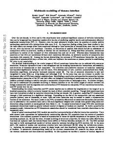
The simulation domain consists of three main regions: i. the continuum region (C) at the centre of the channel, characterised by the macro-scales and governed by the continuous equations (domain above the dashed line in Fig. 1(a)), ii. the molecular/atomistic regions (M) where the particle approach takes place to model fluid/solid interactions at the micro/nano-scales (Fig. 1(b) is an enlargement of one numbered rectangular block drawn in Fig. 1(a)), iii. the overlap region designed to enable the communications between both scales (Fig. 2). To ensure smooth transitions for the macroscopic variables through the overlap region, this zone is subdivided into four smaller layers. From the core flow to the solid boundary, we meet the control layer, the continuum to microscopic C→M layer, the relaxation layer and the microscopic to continuum M→C layer. At the end of the control layer, which is the upper boundary of the molecular region too, a fictive wall is applied to keep constant the number of particles in the molecular domain (incompressible fluid flow). The two layers C→M and M→C are used to exchange the primary variables between the two scales. Notice that the equality of the transport properties in the molecular and continuum regions are necessary to guarantee the flux continuity as well. The part played by the relaxation layer aims to separate the dynamics occurring in the M→C and C→M layers to prevent undesired coupling effects. Further details on the overlap region are presented in Sec. 2.4. Wall or Symmetry L

Inlet HC

z

Outlet H

HM

HM 1

z

2

x

3

HM,f

y

4

HM,w x

Wall (a)

(b)

Figure 1: (a): Scheme of the multi-scale model in a micro-channel of half-height H. The continuum region is governed by the incompressible Navier-Stokes and energy equations (height HC ). A molecular/atomistic description is locally used for the wall and the nearby fluid (height HM ). These two domains are spatially connected thanks to an overlap region (height HO , see Fig. 2). (b): Block of a molecular simulation of height HM . The wall thickness and the fluid height are HM,w and HM,f (HM,w + HM,f = HM ). Periodic boundary conditions are set in x- and y-directions and a specular wall is used to keep constant the number of atoms in the box (bluish top surface). A molecular domain is composed of a x- and y-periodic “block” constituted of a FCC(111) crystalline wall and a chosen density of fluid atoms (Fig. 1(b)). Whereas a narrow single block is clearly well adapted to simulate periodic or established fluid flows like the Couette flow or the mono-dimensional conduction problem, the computational cost becomes prohibitive when the size of the molecular domain increases too much. To get around this issue, in addition to the aforementioned decomposition domain, a partition of the solid boundary is adopted by using nb similar blocks located all along the solid wall (nb = 4 in Fig. 1(a)). Their distribution can be uniform or parametrized by a geometric progression with a scale factor rb . The abscissa xi of the block i is then defined as follows: for i = 1, 2, . . . , nb , !  i−1 1 − r  b   x1 + (xnb − x1 ) if rb 6= 1  1 − rbnb −1 xi = (1)     i−1   x1 + (xnb − x1 ) if rb = 1 nb − 1 The partitioning of the solid wall is, for example, particularly relevant to simulate the development of fluid flows and heat transfer in micro/nano-channels. In this case, the computation cost can eventually be halved by applying symmetry conditions at the centre of the channel.

2.2

Molecular model

The fluid/wall couple used throughout this work is Argon/Platinum (Ar/Pt), whose inter-atomic potentials and the associated parameters are well known in the literature. The Lennard-Jones potential is chosen to model the interactions between two 3

HC

Control layer, ∆z C→M, ∆z HO Relaxation layer, 3∆z/2 N

N

HM,f

N

M→C, ∆z

LM

Figure 2: Example of an overlap region of height HO = 4∆z connecting the molecular domain (black thick lines of total height HM ) and the continuum region partially discretised with blue triangle cells. The overlap region is typically 40% of the fluid molecular height HM,f (see Fig. 1(b)). Microscopic quantities are averaged in the M→C layer (dotted rectangle centred on the middle of the boundary face) and then transmitted to the continuum domain via the boundary conditions (black square symbol). The values at the centres of the other boundary faces (blue triangle symbols) are interpolated from two adjacent molecular blocks. The mean values imposed at the molecular level in the C→M layer are computed by an approximation of the continuum equations (Finite Volume method) at the centre of the layer (the black square symbol). Since the numerical method is based on collocated variables at circumcircle of the blue triangle cell (blue filled circle), second order approximations are used in evaluating the values at the centre of the C→M layer. fluid atoms and a fluid atom with a wall atom. Given the pair distance r, the potential functions are expressed by   σαβ 12  σαβ 6 Vαβ (r) = 4εαβ − , r r where the subscript αβ stands for f f (fluid/fluid) or wf (wall/fluid). The coefficients εαβ et σαβ are respectively the potential well-depth and the “diameter”. Taking argon as the reference material, the potential parameters for the couple Ar/Pt and their atomic masses mf and mw can be expressed in the reduced Lennard-Jones units (all these parameters can be found in Maruyama and Kimura (1999)) εf f = ε,

σf f = σ,

εwf = 0.535 ε,

mf = m

σwf = 0.906 σ,

mw = 4.8833 m

with ε = 1.656 × 10−21 J, σ = 3.405 ˚ A and m = 6.633 × 10−26 kg. The solid wall is modelled with three layers of platinum atoms arranged in a FCC(111) lattice. The distance between two equilibrium positions is 0.814 σ (Sun et al., 2009), what leads to a solid density ρw = 12.76 m/σ 3 (21450 kg/m3 ). To allow the thermal vibrations, each solid atom is connected to its nearest neighbours with springs of stiffness k = 3249.1 ε/σ 2 (Maruyama and Kimura, 1999). The associated harmonic potential is a quadratic function of the atomic displacement measured for the pair distance r between two solid atoms 1 Www (r) = kr2 2 Moreover, two extra layers of “phantom atoms” (Maruyama and Kimura, 1999; Maruyama, 2000) are added below the three layers to model the semi-infinite wall. The lowest layer is kept stationary (fixed atoms) while the upper layer is used to control the temperature of the solid wall through a Langevin thermostat. The potentials and the current positions r1 , r2 , . . . , rN of all the N atoms of the system being known, we are able to determine the force Fi applied to any atom i and its acceleration ¨ri according to Newton’s second law. Typically, the equation of motion 4

for a single atom i of type α (fluid or solid) reads mα ¨ri (t) = Fi (t) := − with Vtot (r1 , r2 , ..., rN ) =

∂ Vtot (r1 , r2 , ..., rN ) ∂ri

(2)

1 X 1 X 1 X Vf f (kri − rj k) + Vwf (kri − rj k) + Www (kri − rj k) 2 2 2 i,j6=i

i,j6=i

i,j6=i

Since periodic boundary conditions are applied in x- and y-directions, an external driving force Fext could be added to mimic the pressure contribution. The total potential Vtot (r1 , r2 , ..., rN ) is composed of three sums, respectively for all pairs of fluid/fluid f f , wall/fluid wf and wall/wall ww atoms. From the practical point of view, it is not necessary to treat all pair interactions: the contributions of pairs in Vtot with distances higher than the cut-off radius rc = 2.5 σ are neglected and not considered in the resulting force computation. The equation of motion (2) is integrated using the Leapfrog-Verlet algop rithm with the microscopic time step δt = 5 × 10−3 τ (Rapaport, 2004), where τ = mσ 2 /ε (2.15 × 10−12 s) is the time scale. Although Eq. (2) constitutes the basic motion equation, some care must be taken for the atoms belonging to the lattice crystal and the atoms located inside the C→M layer (Fig. 2). In the first case, extra forces must be added to maintain the wall at the desired temperature Tw . Using the Langevin thermostat, Eq. (2) must be corrected for the solid atoms of the upper phantom layer as follows: mw ¨ri (t) = Fi (t) − αw r˙ i (t) + Rw i (t), with αw = 168.3 τ −1 (Maruyama and Kimura, 1999; Maruyama, 2000) the damping constant and Rw i a random force vector. w Each independent component of R is sampled from a Gaussian distribution with a zero mean and a standard deviation i p 2αw mw kB Tw /δt, where kB is the Boltzmann constant (kB = 1.38063 × 10−23 m2 kg/s/K). The detailed description of the extra forces to introduce into the equation of motion (2), in order to control the velocity and temperature inside the C→M layer, will be discussed in a section devoted to the coupling between the macroscopic and microscopic scales (see Sec. 2.4.3).

2.3

Continuum approach

The continuum domain is governed by the incompressible Navier-Stokes and energy equations:  ∇·u = 0      Du ρ = −∇p + ∇ · (µ(∇u + (∇u)T )) Dt      ρc DT = ∇ · (λ∇T ) + µ (∇u + (∇u)T ) : ∇u Dt

(3)

where D/Dt stands for the material derivative, and u = uex + wez , p and T are the two-dimensional velocity, the pressure and temperature fields. The quantities ρ, µ, λ and c are the fluid density, the dynamic viscosity, the thermal conductivity and the specific heat. The conditions applied to the physical domain on the top and lateral boundaries will be presented later for each problem, while those enforced at the lower borderline (black square on the blue line in Fig. 2) will be detailed in Sec. 2.4.2. The discrete fields are approximated with a collocated Finite-Volume scheme suitable for some unstructured meshes (Ch´enier et al., 2006, 2008). One important requirement the meshes must fulfil is that the straight line joining any adjacent cell centres must intersect their common face at its gravity centre. For example in two dimensions, the variables can be expressed at the centre of the rectangular cells or at the circumcircles for triangular meshes (Delaunay tessellation). The spatial discretisation of the continuous equations is designed to ensure that the discrete variables satisfy the kinetic and “energy” (L2 -norm) balances similar to the continuous equations. For time dependent problems, a second order Euler discretisation associated with a fully implicit scheme is used. The global algorithm is second order accurate in space and time. The resulting discrete non-linear system is solved with a Newton-Raphson algorithm.

2.4

Spatial coupling method and overlap region

The primary variables, velocity u and temperature T , of the hybrid method must be synchronized in time and space between the Molecular Dynamics and the Finite Volume methods to guarantee a correct coupling and to provide an accurate solution. This is performed by exchanging the macroscopic quantities through the overlap region. The continuity of the associated fluxes is then ensured if the macroscopic transport coefficients µ, λ and the specific heat c are identical in the two domains. From classical thermodynamics laws, the relation between specific heat at constant pressure cp and volume cv is given by: cp − cv =

T (∂p/∂T )2 ρ2 (∂p/∂ρ)

5

with

cv =

∂U ∂T

The pressure p = fp (T, ρ), the internal energy U = fU (T, ρ) and their partial derivatives are computed from the analytical equation of state of the Lennard-Jones fluid by Kolafa and Nezbeda (1994). For an incompressible fluid flow model, the specific heat is given by c = cv = cp . The dynamical viscosity and the thermal conductivity are evaluated from the correlations of Galli´ero et al. (2005) and Bugel and Galli´ero (2008) respectively. The values are in good agreement with those computed via equilibrium or non-equilibrium Molecular Dynamics simulations (Kubo, 1957; Muller-Plathe, 1999; Meier, 2002; Rapaport, 2004) or extracted from the database by Lemmon et al. (2011). Before focusing on the coupling techniques inside the different layers of the overlap region, it is crucial to clearly define the way the mean quantities are calculated from the micro/nano-scales. 2.4.1

Macroscopic quantities and average values

This section briefly introduces the way the macroscopic quantities are calculated from the Molecular Dynamics data. To make easier the presentation of the different averages, a schematic drawing is given in Fig. 3. This figure shows one simplified molecular block domain of rectangular shape, made up of 4 × 6 subcells, at different times (t = t1 , . . . , t4 ) and for three independent but equivalent simulations (same statistical constraints) S1 , S2 and S3 , simply called “samples” thereafter. The spatial average of a quantity Φ, for example over the subcell C(2,3) , for the sample S1 and at time t2 writes S

NC1 (t2 )

hΦiC(2,3) S1 T2 =

2,3 X

, (2) Φi

1 NCS2,3 (t2 )

i=1

1 with NCS(2,3) (t2 ) the number of particles in C2,3 , at time t2 for the sample S1 . Since the number of molecules is often too small to obtain an accurate evaluation of the mean quantities, the latter definition is extended for a Time interval (e.g. hΦiC(4,5) S3 T1−4 in green, Fig. 3) and then for different Samples (e.g. hΦiC(2,4) S1−3 T3−4 in blue, Fig. 3). Therefore, the average of a quantity Φ over one Cell, different Samples and during a Time period (CST ) is defined as follows: Sk

hΦiCST =

(tj ) NS X NT NC X X

(j) Φi

,N N S X T X

(4)

k=1 j=1

i=1

k=1 j=1

NCSk (tj )

where NS is the number of samples, NT the number of discrete temporal iterations and NCSk (tj ) the number of particles contained in cell C at time tj := t0 + (j − 1) δt and for the sample Sk . It is worth pointing out that this writing gives back the usual definitions for averages over space, simply noted hΦiC , over space and time, hΦiCT , and over space for several samples hΦiCS . For example, the instantaneous macroscopic velocity and temperature for the sample S1 , in a cell having N particles are: N 1 X r˙ i (t) u(t) = h˙r(t)iC = N i=1 and T (t) =

2 3kB

2 = 3kB



1 m(˙r(t) − u(t))2 2

 C

N 1 X1 2 m (˙ri (t) − u(t)) N i=1 2

!

Another kind of average technique is often used in the literature as well. It consists in computing the mean fluid velocity by measuring the mean particle velocity in a cell, and then averaging this mean over the different samples. But for systems far from equilibrium, such as those submitted to large temperature or velocity gradients, a bias can arise with this latter definition, contrary to the formula given in Eq. (4) (Tysanner and Garcia, 2004). 2.4.2

From molecular to continuum: M→C layer

The velocity uM→C and temperature TM→C are calculated by averaging over a time interval q δt and over all samples. Typically, q is the total number of time steps between two successive M→C exchanges. For unsteady problems, qδt = ∆t the time step of the macroscopic model. Using the definitions presented in Sec. 2.4.1, the explicit expression for uM→C reads uM→C = h˙riCST where the averaging cell is the M→C layer. In the same way, the temperature TM→C is   2 1 2 TM→C = m (˙r − uM→C ) 3kB 2 CST 6

average over space, at time t2 , for sample S1 , in cell (2,3) hΦ(t2 )iC(2,3) S1 T2

average over space & time, for sample S3 , in cell (4, 5) hΦiC(4,5) S3 T1−4

t1 t2

S3 t3

S2 t4

average over space, time & all samples in cell (2,4)

S1

t

hΦiC(2,4) S1−3 T3−4

Figure 3: Graphical representation of three kinds of averages. One schematic molecular block is drawn at 4 times (t1 , · · · , t4 ) and for 3 samples (S1 , S2 , S3 ). This block is also partitioned into 4 × 6 rectangular sub-domains. Averages can be calculated as a function of space (over one or more subdivisions of the domain), time or samples, or any combinations of these variables. The macroscopic variables uM→C and TM→C are used to define the lower boundary conditions of the continuum domain. When the M→C layer is centred on the edge node of the Finite Volume method (black square in Fig. 2), the average values are directly applied; otherwise, values on the other boundary nodes (blue triangles in Fig. 2) are evaluated through a linear interpolation between two successive molecular blocks. 2.4.3

From continuum to molecular: C→M layer

The velocity uC→M and temperature TC→M are computed by means of the Finite Volume approximation of the Navier-Stokes and energy equations (3). Then, to feed these variables back into the Molecular Dynamics domain, the equation of motion k (2) is modified for the NCSC→M (tj ) particles lying in the C→M layer, at time tj and for the sample Sk as follows. First, the constrained dynamics is used to impose a linear profile (Sun et al., 2010): m¨r?i (t) = Fi (t) − hF(t)iCC→M S + ξ


 m [[uC→M ]] (z) − h˙r(t)iCC→M S (z) δt

(5)

with ¨r?i (t) the intermediate acceleration, Fi the force which derives from Eq. (2) and [[ · ]] (z) stands for a linear operator such that    2(z − zf )  h˙r(t)iCC→M S (z) := h˙r(t)iC 0 0 S + h˙r(t)iCC→M S − h˙r(t)iC 0 0 S C →M C →M ∆z and 2(z − zf ) [[uC→M ]] (z) := uf + (uc (t) − uf (t)) ∆z where uc and uf are macroscopic velocities respectively located at the centre (ordinate zc ) and at the middle of the bottom face (ordinate zf ) of the C→M layer (see Fig. 4 for the notations). This latter point is also the centre of a new layer noted C’→M’. The values uc and uf are extrapolated from the Finite Volume approximation of the velocity and its gradient evaluated at the nearest collocation point xK to the centre of the C→M layer. The value of the damping coefficient ξ in Eq. (5) must be chosen carefully. A too small value does not constrain enough the velocity while a too large value could have undesired effects on the temperature field. Based on previous studies, where ξ is either fixed (O’Connell and Thompson, 1995) or related to the number of microscopic iterations q in the coupling algorithm (Sun et al., 2009), the value ξ = 2 × 10−2 is chosen in this work. In addition to the aforementioned driving force, which manages the mean velocity of the particles, the temperature is controlled at the desired value by means of the Langevin thermostat (Sun et al., 2009, 2010):  
m¨ri (t) = m¨r?i (t) − mαf r˙ i (t) − h˙r(t)iCC→M S (z) + Rfi (z, t) (6) 7

with αf = 1 τ −1 the damping coefficient and Rfi (z, t) p a force whose components are sampled into a Gaussian distribution of zero mean value and with the standard deviation 2αf m kB [[TC→M ]] (z)/δt. The targeted linear temperature profile [[TC→M ]] (z) is approximated similarly to the above velocity. Besides the velocity and temperature, the pressure gradient (∂x p)K ≈ (∂x p)(xK ) could be transferred from the Finite Volume T approximation to the molecular region as an external driving force Fext = (−m/ρ (∂x p)K ; 0; 0) in equation of motion (2) and applied on all unconstrained fluid molecules. For the sake of clarity, the notations are abridged in the remaining of the presentation by suppressing both the double brackets and the z-dependency for the variables, for example uC→M := [[uC→M ]] (z) and TC→M := [[TC→M ]] (z).

z

xK zc zf

C→M, ∆z

N

C0 →M0 , ∆z

Figure 4: Enlargement of the overlap region in Fig. 2 around the C→M layer. An extra layer labelled C0 →M0 , of height ∆z and centred on the bottom face of the C→M layer (triangle symbol), is introduced in order to manage the dynamic and thermal constraints in the molecular domain C→M. The velocity and temperature values at the ordinate zf and zc result from the macroscopic variables and their gradients at the collocation point xK (blue filled circle), namely the circumcenter of the control volume (blue filled triangle).

2.4.4

Upper bound of the overlap region

Since the upper limit of the overlap region (and molecular domain) is physically unbounded, a fictive specular wall is used to prevent atoms from going, and thus to conserve the total number of particles in the domain which ensures that the density in the both approaches is the same. Whenever an atom crosses this boundary, it is re-inserted immediately at the same location with its normal velocity component inverted. However, the presence of this fictive wall can be the cause of undesired effects, which translate into a non physical organization of the molecules at the vicinity of the boundary, in the form of inhomogeneous distributed atoms in adjacent and parallel layers. To reduce efficiently these spurious oscillations, a boundary force F w (rw ) is added in the equation of motion (2) (Werder et al., 2005): m¨ri (t) = Fi + F w (rw )ez

(7)

This force, function of the distance rw between the particle i and the upper boundary, represents the effect exerted by the ghost atoms located outside the molecular domain on particle i. Its expression, written in terms of radial distribution function g(r) and fluid/fluid potential Vf f (r), is given by Z rc Z √rc2 −z2 ∂Vf f (r) x F w (rw ) = −2πρ g(r) xdxdz (8) ∂r r z=zm x=0 with zm = min(rc , rw ) and (x, z) the local cartesian coordinates centred on the fluid particle. The radial distribution function g(r) is evaluated through an analytical expression (Morsali et al., 2005) at the temperature [[TC→M ]] (zc ). This wall force is pre-calculated once at each coupled iteration, as follows. At first, F w (rw ) is evaluated on a spatial fine grid defined with j 200 nodes over the range [0; rc ]. Then for any node j = 1, · · · , 200, F w (rw ) is approximated with the second order rectangle method (midpoint rule). The resulting approximation is in very good agreement with the correlations proposed by Werder et al. (2005). 8

2.5

Temporal or iterative coupling

In the hybrid method, the synchronization between the micro and macro-scales depends on the transient or stationary nature of the problem studied. For an unsteady flow, the microscopic and macroscopic time steps are linked in order to achieve the temporal coupling between the two approaches: ∆t = qδt, q ∈ N?,+ , with a typical value of q = 100. A synthetic description of the hybrid time stepping scheme is shown in Fig. 5. The first key point is that the temporal integration periods of the continuous and molecular models are staggered by a half macroscopic time step ∆t/2. Assuming that the positions and velocities of all particles are known at time tn+1/2 , the temporal evolution in the microscopic domain is performed by integrating the Newton’s second law from tn+1/2 to tn+3/2 with the imposed macroscopic values evaluated at time tn in the C→M layer: (n)

(n)

(n+1)

(n+1)

uC→M and TC→M . Afterwards, the macroscopic variables are solved at time tn+1 with boundary conditions uM→C and TM→C calculated with averages h · iCM→C ST(n+1/2)−(n+3/2) . tn−1

tn+1

tn

tn+2

C

(u ,T

∆t

) (n) C→

M

(n+1)

(u, T )boundary = (u, T )M→C

Given quantities qδt = ∆t

Constrained dynamics in C→M region

M tn− 1 2

tn+ 1 2

tn+ 3 2

Figure 5: Temporal coupling in the hybrid scheme. All quantities greyed are assumed to be known. During the temporal integration at molecular level (M) between tn+1/2 and tn+3/2 , the dynamics is constrained in the C→M layer (Fig. 2) so that the averaged microscopic velocity and temperature converge to the corresponding macroscopic variables stemming from the (n) continuum region (C) at time tn : (u, T )C→M . Then the averaged velocity and temperature calculated at time tn+1 in the M→C layer, (u, T )M→C , are forwarded to the continuum domain to impose the macroscopic boundary conditions at time tn+1 .

For steady flows, the coupling between the microscopic and macroscopic models is still iterative, but without any temporal synchronization. Let us assume that the macroscopic boundary conditions are known at iteration k. Then the approximated velocity and temperature fields uk and T k are solutions of the discrete Navier-Stokes and energy equations (3) written in their stationary form (time derivatives dropped). Once the steady solution is achieved, the Newton’s second law is integrated for the particles over a period qδt with the imposed macroscopic values ukC→M and TCk→M in the C→M layer. The number q of molecular time steps increases substantially, from about 20 000 to 1 000 000, depending on the maximal relative difference between two iterations of the coupling macroscopic variables, namely max(C,ξ) (ξCk−1 /ξCk − 1) with C ∈ {C→M; M→C} and ξ ∈ {T, u}. Finally, the new boundary conditions of the macroscopic model at the new iteration k + 1 is updated from the atomistic level. This iterative coupling is shown to be more efficient than a temporal coupling, provided that the steady solution is solely sought.

2.6

Initialization step: analytical hybrid model

The hybrid simulation of steady or unsteady problems requires a coherent initialization of the solution, both in the molecular and continuum domains. For example, when the initial solution is isothermal at rest, the mean velocity is zero and the temperature is controlled at the chosen value. Whereas these conditions are easily performed in the continuum domain, more attention must be paid on the molecular region. Firstly, the fluid molecules are arranged in a cubic crystalline pattern, with their velocity components drawn in a Gaussian distribution of zero mean value. Then, the equations of motion (2) are integrated in time with the Berendsen thermostat (Berendsen et al., 1984) applied on the whole fluid particles until the equilibrium is reached. Despite the relevance of the isothermal solution at rest as an inital condition, it could be more suitable to choose more complex temperature and/or velocity profiles, for example to improve the speed of convergence towards a steady solution. The main issue is then to initialize the hybrid solution efficiently, namely by minimizing the computational cost. To to this, we are going to introduce a variant of the hybrid scheme in which the expensive molecular dynamics is substituted by two analytical profiles, one for the horizontal velocity component and the other for the temperature. The resulting method is simply called analytical hybrid method. The analytical solutions must fulfil either the velocity slip or temperature jump

9

conditions at the wall, and the passed values in the C→M layer. The simplest functions are polynomials of degree 1 or 2, depending on whether one or two points are used in the overlap region (zc or zc and zf , see Fig. 4). Once the analytical hybrid solution has converged, the dynamics of the fluid particles must be driven in order that the average velocity and temperature correspond to the computed polynomial profiles. This step is similar to the method described for the C→M layer (see Sec. 2.4.3): the whole of the molecular fluid domain is split into 10 to 20 sub-layers in which the particle motion is integrated with a Langevin thermostat adjusted to control the local temperature at the desired values. To illustrate the iterative procedure of convergence of the analytical hybrid method, the stationary no-slip Poiseuille flow is simulated with linear and quadratic approximations (Fig. 6). It is worth noticing that the coupling algorithm is basically 1

u/umax

u/umax

ns

M→C

0.6

0.4

0.4

0.2

0.2

0

atio iter

0.6

pled

M→C

0.8 C→M

0.8

Analytical Poiseuille Quadratic model in M region Navier-Stokes in C region

coupled iterations

cou

Analytical Poiseuille Linear model in M region Navier-Stokes in C region

C’→M’ C→M

1

0 0

0.1

0.2

0.3

0.4

0

0.5

z/H

0.1

0.2

0.3

0.4

0.5

z/H

(a)

(b)

Figure 6: Iterative convergence of the coupling algorithm for the analytical hybrid method with a single block and HM,f /HC = 1. (a) Linear approximation. (b) Quadratic approximation. The first 5 and last 3 iterations are drawn, only. the same for the standard hybrid method and the analytical hybrid method: communications between the core region and the block domain still occur in the overlap region, but the averaged values are substituted by the analytical values. The coupling algorithm is carried out iteratively until the steady-state, i.e for a maximal relative increment of the primary variables transferred inside the C→M and M→C layers less than 0.1%. For the ratio HM,f /HC = 1, the stationary solution is reached after 56 iterations for a second order polynomial and 17 iterations for a linear approximation. Whereas the quadratic model provides a 1% accurate solution to the exact parabolic profile over the whole computation domain (Fig. 6(b)), this relative difference reaches 24% in the linear case (Fig. 6(a)). However in the spirit of the molecular hybrid method, the ratio HM,f /HC must remain small enough in order to neglect the average vertical velocity component in the M→C layer. Thus, if this ratio is set to 1/25, the linear model converges within 11 iterations only, and the analytic hybrid solution departs from about 0.2% of the Poiseuille profile. Given the number of iterations and the stopping criterion of the iterative coupling, the choice of a linear approximation inside the block domain seems to be the better compromise between the accuracy and the computational cost.

3

Results of the hybrid method

Before addressing in details the hybrid method with multiple molecular blocks, classic test problems with a unique coupling region are handled.

3.1

Validation for a single molecular block

In this section, the solutions are unsteady, one dimensional and the domain is simulated over the total height H. The lengths of the continuum and fluid particle domains are identical, HC = HM,f = 119.695 σ, what leads to H = HC + HM,f − HO = 191.512 σ (65.2 nm) with an overlap region HO = 40% HM,f . The transversal dimensions of the molecular block are Lx × Ly = 9.8763 σ × 9.775 σ. The molecular region contains N = 9360 atoms of Argon in√liquid phase, ρ = 0.81 m/σ 3 3 (1360.95 kg/m macroscopic coefficients evaluated at T = 1 ε/kB (120 K) are µ = 2.136 mε/σ 2 (1.931 × 10−4 Pa · s), √ ). The 2 λ = 6.721 kB mε/σ (1.265 × 10−1 W/m/K) and c = 2.402 kB /m (4.999 × 102 J/kg/K). The continuum region is covered with a triangular Delaunay tessellation based on the discretisation of the horizontal and vertical boundaries into 8 and 40 uniform segments respectively. The ratio between the continuum and molecular time steps is q = 150. The macroscopic variables stemming from the molecular dynamics are calculated according to Eq. (4) in 10 10

vertical sub-domains of length HM,f /10, during one macroscopic time step ∆t = qδt (NT = q) and for the whole of the independent samples (NS = 40). To limit the velocity and temperature jumps occurring at the fluid-wall interface, the atomic wall is substituted by a stochastic wall model: when a particle crosses the interface plane, it is re-inserted with a velocity whose the tangential and normal components are sampled from a Gaussian and Rayleigh distributions respectively, with zero mean values and standard deviations corresponding to the wall temperature Tw . The first validation test concerns the transient Couette flow between two parallel plates. After an equilibration period at the wall temperature Tw = 1 ε/kB , the upper plate in the continuum region is suddenly set in motion at a constant horizontal velocity u0 = 1 σ/τ (158.03 m/s), while the lower wall in the atomic region stays at rest. In order to keep constant the macroscopic transport coefficients in both continuum and molecular domains and to limit the heat production due to the viscous dissipation, the temperature in the whole system must be controlled close to the wall temperature Tw at which µ, λ and c are evaluated. To that purpose, the temperature in the C→M layer is kept to TC→M = Tw . Figure 7(a) shows the normalized x-velocity u/u0 as a function of the reduced height z/H, and for different time intervals (τ1 –τ2 ). Empty and filled circles stand for molecular and continuum hybrid solutions, while the continuous line represents the mean analytical velocity profile 1 u(z) = u0 τ2 − τ1

Z

τ2

τ1

    ∞ z 2 X (−1)k kπz µk 2 π 2 t dt + sin exp − H π k H ρH 2

(9)

k=1

obtained by solving the isothermal Navier-Stokes equations with no-slip boundary conditions at walls. The hybrid and analytical solutions match very well. The relative difference is very small (less to 1% in L2 norm). The discrepancy is essentially due to the calculation of the macroscopic field in the molecular domain. This could be reduced by improving the calculations of the averages, either with additional samples or molecules in the y-direction (Ly is then also modified according to the desired density). The efficiency of the coupling algorithm is also visible in the overlap region where the solutions achieved by two approaches are very close to each other (z/H ∈ [0.36; 0.56]). The second test case is the transient thermal conduction problem with stationary walls. After an initialization step devoted to the computation of the equilibrium state at Tw = 1 ε/kB (120 K), the temperature of the upper plate is suddenly increased to T2 = 1.5 ε/kB (180 K), while the temperature of the bottom plate is kept at T1 = Tw . In the C→M layer, the mean velocity uC→M is set to be zero during the simulation to avoid the appearance of a spurious velocity. Macroscopic coefficients are evaluated at the intermediate temperature (T1 + T2 )/2. Similarly to the Couette flow problem, the hybrid and analytical reduced temperatures T (z)/T1 are shown in Fig. 7(b) as a function of the dimensionless height z/H, and for different time intervals. The expression of the analytical solution is identical to Eq. (9), provided that the reduced velocity is replaced by (T (z) − T1 )/(T2 − T1 ) and the kinematic viscosity is substituted by the thermal diffusivity coefficient α = λ/(ρc). Again, the hybrid results are in very good agreement with the analytical solution. 1.5

1 (0-45) τ (45-180) τ (180-600) τ (600-1500) τ (1500-6000) τ

0.8

1.3 T/T1

0.6 u/u0

(0-45) τ (45-180) τ (180-450) τ (450-1125) τ (1125-6000) τ

1.4

0.4

1.2

0.2

1.1

0

1 0

0.2

0.4

0.6

0.8

0

1

0.2

0.4

0.6

0.8

1

z/H

z/H

(a)

(b)

Figure 7: (a) Mean velocity u(z/H)/u0 and (b) temperature T (z/H)/T1 profiles for different time intervals. Continuous curves indicate the analytical solutions, filled and empty symbols stand for continuum and particle solutions of the hybrid method. The half lengths of the error bars represent the standard deviations and illustrate the scattering of the spatiotemporal averages over the NS = 40 independent samples.

11

3.2

Hybrid scheme for multiple molecular blocks

The aim of this section is to validate our hybrid method to simulate multi-scale fluid flows and heat transfer. As a significant test case, we are interested in computing the hydrodynamic development of a fluid flow in the entrance region of a channel of height 2H and length L  2H, using several molecular blocks to model the fluid/wall interaction at the atomic level. For symmetry purpose, only the half height H of the channel is simulated (see Fig. 1(a)). The atomic wall is maintained isotherm at T = Tw . The fluid enters into the channel at the wall temperature Tw , with a velocity profile u(z), and the flow is assumed fully developed at the outlet. The ratio between the heights of the fluid molecular domain and continuum domain is set to HM,f /HC = 1/25. The computations have been carried out for HM,f = 99.44 σ leading to H = 2545.6 σ (866.8 nm). The length and the wall temperature are L = 4000 H (3.46 mm) and Tw = 1.1 ε/kB (132 K). The continuum region of height HC is discretised in Nx × Nz = 48000 × 30 rectangular control√volumes with refined cells near the inlet and √ close to the wall. The macroscopic coefficients evaluated at Tw are µ = 2.073 mε/σ 2 (1.874 × 10−4 Pa · s), λ = 6.832 kB mε/σ 2 (1.285 × 10−1 W/m/K) and c = 2.375 kB /m (4.945 × 102 J/kg/K). To compare efficiently the solution of the hybrid scheme and the one arising from the pure Finite Volume approach on the full half-height of the channel, the inlet velocity profile must cancel at walls. A parabolic boundary layer profile u(z)/u0 = z(2δ − z)/δ 2 is then chosen in the vicinity of the wall for 0 ≤ z ≤ δ, connected to a uniform velocity profile in the core region for δ ≤ z ≤ H. In our simulation, u0 = 1 σ/τ (158.03 m/s) and δ = 0.2H. The resulting Reynolds number, based on the half-height H, is Re ≈ 1000, less than the linear critical Reynolds value Rec = 5780 for the plane Poiseuille flow (Thomas, 1953).

3.2.1

Distribution of the molecular blocks

Since the number of the molecular blocks and their position play a key role in the accuracy of the hybrid solution, these parameters must be systematically investigated. To perform such studies at a reasonable CPU-cost, the analytical hybrid scheme (Sec. 2.6) with no slip velocity and temperature jump at the solid wall is chosen. The hybrid solution is compared to the Finite Volume solution computed on the same structured grid at which a unique row of 48000 cells is added to cover the molecular domain of height HM,f .To measure the discrepancies between both solutions, the relative errors in L2 -norm are calculated in the entrance region (for x ≤ 50H) and in the whole domain. For a uniform distribution of the blocks along the channel (Fig. 8), about nb = 20 blocks are required to achieve a 1% relative error in the whole domain. But this measure is not really appropriate since velocity field strongly evolves in the entrance region before becoming almost independent of the axial coordinate in the fully developed region. If we consider the deviation of the solutions in the entrance region, the disparity increases significantly. To keep a relative error less than 1%, nb = 200 blocks are now necessary. From nb ≈ 2000, the relative error of the velocity field saturates slightly above 0.1%, a value which corresponds to the error of the coupling algorithm for a Poiseuille flow with a single block of height ratio HM,f /HC = 1/25 (see Sec. 2.6). It is interesting to remark that the number of coupling iterations remains close to 10 for a stopping criterion based on the relative difference between the exchanged values in all the overlap regions less than 0.1%, whatever the number of blocks used in the simulation. Once the number of blocks is determined, the initialization and then the simulation with the molecular hybrid scheme can start. However, it is clear that such simulation with hundreds blocks is far to be feasible: whereas a steady solution achieved with the Finite Volume method costs few minutes, the molecular simulation on each block takes several CPU days. Hence, the minimization of the number of blocks is a fundamental issue to hope obtaining the stationary solutions in a acceptable human time, using about hundred cores in parallel. Therefore, to keep a realistic CPU-time, the number of blocks must not exceed nb = 20. Given this restrictive condition, it is necessary to modify the block distribution along the wall in order to optimize their arrangement. Figure 9 shows the relative error of the velocity and temperature between the analytical hybrid method and the reference solution as a function of the block distribution defined by the common ratio rb (Eq. (1)). The deviation from the Finite Volume solution is clearly larger for the velocity than the temperature. Moreover, the maximal discrepancies are mainly located in the entrance region (encapsulated frames in Figs. 9(a) and 9(b)). On the whole, the optimal common ratio increases with the decrease in the number of blocks nb . The slopes of the curves also indicate that overestimating the common ratio rp produces a much smaller deviation than an underestimation would do. 3.2.2

Multi scale fluid flow and heat transfer simulation

A number of 8 identical molecular blocks is adopted. They are distributed according to a geometric progression, with a common ratio fixed to rb = 4 (Fig. 9). Each block, of dimensions (Lx ; Ly ; HM,f ) = (9.87; 9.77; 99.44) σ, is composed of 7776 argon atoms to capture the fluid/solid interactions along the x-direction. The steady state is obtained by solving the equations of system (3) where the temporal derivatives are disregarded. The initialization of the iterative process is carried out with the analytical hybrid method. As indicated in the third column (LM) in Tab. 1, the initial field departs from less than 0.5% to the Finite Volume solution (second column) on the whole of cross sections corresponding to the 8 blocks. The velocity and temperature profiles presented in Figs. 10 and 11 are averaged over 1 million of microscopic time steps

12

-1

10

10

-1

u T

-1

nb 10

-2

-2

10

errL2

10

10

-3

-4

10

-1

100

1000

10000

nb

-3

10

10

100

1000

10000

nb

Figure 8: Relative deviations over the whole fluid domain of the velocity and the temperature between the analytical hybrid and the Finite Volume methods, as a function of the number of blocks nb uniformly distributed. The encapsulated figure shows the relative deviations calculated in the inlet region, i.e. for x/H ≤ 50.

-1

-1

-1.5

-10

-3

-2

0

0.2

0.4

0.6

3/4 0.8

1

nb

-2

-2.5 -3

-10

slope slope

-2

slope

-2

-2.5

-1.5

nb = 4 nb = 6 nb = 8 nb = 10 nb = 12 nb = 14 nb = 16

-1.5

log10(errL2(T))

-1.5

log10(errL2(u))

-1

nb = 4 nb = 6 nb = 8 nb = 10 nb = 12 nb = 14 nb = 16

5

slope 3/

-3.5 -4

0

0.2

0.4

0.6

0.8

1

nb

-2.5

-2.5 -3

-3

0

0.2

0.4

0.6

0.8

-3.5

1

log10(rb)

0

0.2

0.4

0.6

0.8

1

log10(rb)

(a)

(b)

Figure 9: Relative deviations of (a) the velocity and (b) the temperature between the analytical hybrid and the Finite Volume methods, as a function of the geometric progression of the common ratio rb (Eq. (1)) and the number of blocks nb . The encapsulated frames show the relative deviations calculated in the inlet region, i.e. for x/H ≤ 50.

δt = 5 × 10−3 τ , and calculated with NS = 128 samples. As in Sec. 3.1, a stochastic wall model is first adopted to reduce as much as possible the velocity and temperature jumps, and then to perform comparisons with the solution achieved by the Finite Volume approximation. Figures 10(a) and 10(b) show the velocity and temperature profiles in the cross sections corresponding to the abscissa of the different blocks. The solutions of the particle and continuum regions for the hybrid scheme are presented with empty and filled circles, respectively; the Finite Volume solution is drawn with continuous lines. As can be seen in the different enlargements, the couplings into the overlap region work well. The velocity and temperature fields between the hybrid and Finite Volume solutions are in very good accordance, respectively less than 0.5% and 1% (Tab. 1, forth column labelled SW). Let us now study the fluid flow and heat transfer when the wall is modelled by a crystalline pattern. Thus, in addition to the 7776 argon atoms, 840 platinum atoms make up the wall. These atoms are organized in a face-centred cubic crystalline lattice, closely packed in parallel layers to the diagonal plane (FCC(111)). The velocity and temperature profiles are shown in Fig. 11 in the different slices corresponding to the positions of the 8 molecular blocks. The heigh H still denotes the gap between the wall and the channel axis (see Fig. 1(a)). The z-axis origin coincides with the top layer of the atomic wall. The velocity discrepancy, stemming from the simulations performed with the stochastic wall (Fig. 10(a)) and the atomic wall (Fig. 11(a)), appears to be very small. This observation is confirmed by the calculation of the relative differences between the maximal velocities in the different block sections which do not exceed 0.1% (Tab. 1, fifth column labelled AW). On the other

13

1.2

1.5 x/H = 0 x/H = 0.732 x/H = 3.662 x/H = 15.38 x/H = 62.25 x/H = 249.7 x/H = 999.8 x/H = 4000

1.25

x/H = 0 x/H = 0.732 x/H = 3.662 x/H = 15.38 x/H = 62.25 x/H = 249.7 x/H = 999.8 x/H = 4000

1.15

1

1.03

1.02

T/Tw

u/u0

0.4

0.75 0.3

0.5

1.1 1.01

1

0.2

1.05

0

0.01

0.02

0.03

0.04

0.05

0.06

0.1

0.25 0 0

0

0

0.2

0.02

0.4

0.04

0.8

0.6

0.06

1 1

0

0.2

0.4

0.8

0.6

z/H

1

z/H

(a)

(b)

Figure 10: (a) Velocity and (b) temperature profiles for the fluid flow and heat transfer in a long channel for a stochastic wall. The 8 profiles are drawn at the molecular block abscissa. The empty and filled symbols stand for the hybrid solution in the particle and continuum domains, respectively. The continuous lines represent the standard Finite Volume approximation.

block No. 1 2 3 4 5 6 7 8

Finite Volume (FV) u/u0 T /Tw 1.000 1.002 1.006 1.019 1.042 1.034 1.129 1.043 1.295 1.058 1.397 1.096 1.399 1.167 1.399 1.180

Linear Model (LM) u/u0 (e/FV ) 1.000( 0.0%) 1.005(-0.1%) 1.041(-0.1%) 1.130(-0.1%) 1.299(-0.3%) 1.395(-0.2%) 1.397(-0.1%) 1.397(-0.1%)

T /Tw (e/FV ) 1.000(-0.2%) 1.018(-0.1%) 1.033(-0.1%) 1.043( 0.0%) 1.059( 0.1%) 1.099( 0.3%) 1.172( 0.4%) 1.186( 0.5%)

Stochastic Wall (SW) u/u0 (e/FV ) 1.000( 0.0%) 1.005(-0.1%) 1.039(-0.3%) 1.124(-0.4%) 1.290(-0.4%) 1.392(-0.4%) 1.396(-0.2%) 1.395(-0.3%)

T /Tw (e/FV ) 1.001(-0.1%) 1.016(-0.3%) 1.029(-0.5%) 1.038(-0.5%) 1.052(-0.6%) 1.089(-0.6%) 1.157(-0.9%) 1.170(-0.9%)

Atomic Wall (AW) u/u0 (e/SW ) 1.000( 0.0%) 1.005( 0.0%) 1.038( 0.0%) 1.123(-0.1%) 1.289(-0.1%) 1.390(-0.1%) 1.394(-0.1%) 1.393(-0.1%)

T /Tw (e/SW ) 1.009(0.9%) 1.028(1.2%) 1.046(1.7%) 1.054(1.5%) 1.066(1.3%) 1.104(1.4%) 1.182(2.2%) 1.199(2.5%)

Table 1: Reduced x-velocity at z = H and maximum temperature on block slices for the basic Finite Volume approximation (FV), the linear model (LM) used in the hybrid method for initialization and the molecular hybrid solution with stochastic (SW) or atomic walls (AW). The notation e/ref stands for the relative difference to the reference solution. hand, the relative gaps between the temperature profiles presented in Figs. 10(b) and 11(b) are clearly more significant, up to 2.5% (Tab. 1), because of the temperature slip at the solid/fluid interface. The conservation of the mass flux should be satisfied through each channel cross section which consists of the core flow region and the domain close to the fluid/wall interface. In the present hybrid method, only the mass flow rate in the bulk is explicitly resolved by the second order Finite Volume scheme. However, the global mass flow rates reported in Tab. 2, for both the linear model and the atomic/continuum hybrid method, deviate from less than 0.3% of Q0 , the analytical flow rate based on the inlet velocity profile. These relative differences are clearly negligible, what demonstrates the reliability of the present hybrid method. Let us focus on the results obtained with the atomic wall in order to examine more thoroughly the temperature and the fluid flow at the solid interface. Figure 12(a) presents the normalized velocity slip and temperature jump as a function of the reduced axial coordinate. The velocity slip decreases from 2.25% of the reference inlet velocity u0 to about 0.75% for x/H & 60. From x/H ≈ 250, the flow velocity is fully developed as it is shown in Fig. 11(a) where the different velocity profiles are perfectly superimposed. The temperature jump, normalized with respect to the wall temperature Tw , increases in the entrance region from 1% in the inlet section to 3.25% at x/H ≈ 3.5. Then, it gradually decreases to reach about 2% close to x/H = 60 before increasing again to about 2.8% and remaining almost constant from x/H = 1000 to 4000. If we are interested in the temperature variations, the temperature jump should rather be related to the maximal temperature gap in the channel. In that case, the percentages presented here-above must be multiplied by 5: the temperature jump then varies from about 5% to 15%, what is far to be negligible (see Fig. 11(b)). The dynamical (thermal) slip length Ls−u (Ls−T ) is defined as the distance inside the wall at which the extrapolated fluid

14

1.2

1.5 x/H = 0 x/H = 0.732 x/H = 3.662 x/H = 15.38 x/H = 62.25 x/H = 249.7 x/H = 999.8 x/H = 4000

1.25

x/H = 0 x/H = 0.732 x/H = 3.662 x/H = 15.38 x/H = 62.25 x/H = 249.7 x/H = 999.8 x/H = 4000

1.15

1

1.07 1.06 1.05

T/Tw

u/u0

0.4

0.75 0.3

1.04

1.1

1.03 1.02 1.01

0.5

0.2

1

1.05

0

0.01

0.02

0.03

0.04

0.05

0.06

0.1

0.25 0 0

0

0

0.2

0.02

0.4

0.04

0.06

0.8

0.6

1 1

0

0.2

0.4

0.6

z/H

0.8

1

z/H

(a)

(b)

Figure 11: (a) Velocity and (b) temperature profiles for the fluid flow and heat transfer in a long channel for an atomic wall. The 8 profiles are drawn at the molecular block abscissa. The empty and filled symbols stand for the hybrid solution in the particle and continuum domains, respectively.

block No. 1 2 3 4 5 6 7 8

Linear Model (LM) Q/Q0 − 1 -0.12% -0.14% -0.18% -0.21% -0.23% -0.24% -0.24% -0.24%

Stochastic Wall (SW) Q/Q0 − 1 -0.12% -0.13% -0.17% -0.20% -0.22% -0.23% -0.23% -0.23%

Atomic Wall (AW) Q/Q0 − 1 -0.10% -0.13% -0.15% -0.19% -0.22% -0.23% -0.23% -0.23%

Table 2: Relative error to the analytical flow rate Q0 = 2.630 × 10−4 m3 /s/m in the cross sections of the 8 blocks for the linear hybrid model (LM) and the atomistic/continuum hybrid method with a stochastic (SW) or an atomic wall (AW). velocity (temperature) would equal the wall’s velocity (temperature): Ls−u ≡

−us , ∂u/∂z|z=0

Ls−T ≡

Tw − Ts ∂T /∂z|z=0

Figure 12(b) shows the variations of the reduced slip lengths Ls−u /H (left ordinate) and Ls−T /H (right ordinate) as a function of x/H. In accordance with the preceding results, Ls−u /H is very small, about 2.7 × 10−3 ± 5%, and nearly constant all along the channel flow. In the entrance section (the first molecular block), the reduced temperature slip length is negative, what is a accordance with the weak decreasing temperature profile drawn in red colour in the sub-figure 11(b). This surprising and unexpected result is currently not completely clear. The explanation could be related to the inlet boundary conditions. Indeed, the combined choice of a non uniform velocity profile and a temperature kept uniform at Tw is probably incompatible because of the heat source produced by shear stress which should increase the temperature beyond Tw . From the second block at x/H = 0.732, Ls−T /H becomes positive and ranges between 7.5% to 12.5%, what confirms that the relative jump for the temperature is much higher than for the velocity.

4

Conclusion

In this paper, we have developed a multi-scale approach to solve the fluid flow and heat transfer in micro/nano-channels. The numerical method is based on an atomistic-continuum hybrid scheme which couples the Molecular Dynamics to simulate the complexity of the interactions occurring between the wall/fluid atoms, and the Finite Volume approximation in the core fluid region. To capture the variations of the macroscopic quantities in the channel, a set of small molecular dynamics blocks is distributed all along the wall/fluid interface.

15

4% 0.29%

20%

us/u0 ∆Ts/Tw

Ls-u/H Ls-T/H

3%

y-axis

0.28%

10%

0.27%

0%

0.26%

-10%

2%

1%

y-axis

0% 0.01

0.1

1

10 x/H

100

1000

0.25%

10000

(a)

0.01

0.1

1

10 x/H

100

1000

-20% 10000

(b)

Figure 12: Simulation of the fluid flow and heat transfer with the hybrid method based on an atomic wall. (a) Dimensionless slip velocity us /u0 and temperature jump ∆Ts /Tw at the fluid/wall interface as a function of the reduced abscissa x/H. (b) Dimensionless velocity and temperature slip lengths as a function of x/H. These values were deduced from a linear interpolation of the mean values in the molecular domain over the range 0 < z < HM,f /5. The half lengths of the error bars represent the standard deviations of the interpolation coefficients (rough indication of the confidence interval).

The validity of the multi-scale coupling is shown through comparisons with analytical solutions for two transient test cases: the Couette flow and the heat transfer problems between two parallel plates. On the basis of the so called “analytical hybrid” method used to initialise the hybrid solution, as the number of iterations to achieve the convergence as the number and distribution law of the molecular blocks are studied. The hybrid method has been successfully applied to simulate the fluid flow in liquid phase and heat transfer in a long micro-channel, for stochastic and atomistic walls. In this latter situation, the slip velocity, the temperature jump and the dynamic and thermal slip lengths are studied as a function to the distance from the inlet section. Whereas the slip velocity is clearly negligible, the temperature jump ranges between 5% to 15% of the maximal temperature gap produced by the viscous stresses. The thermal slip length is nearly constant, about 10% of the channel half-height, except in the inlet section where it seems to turn out to be negative.

Acknowledgements This work has benefited from a French government grant managed by ANR within the frame of the national program Investments for the Future ANR-11-LABX-022-01. The authors also thank the Institute for Development and Resources in Intensive Scientific Computing (IDRIS/CNRS) for their support for the project i20142b7277.

References M. Allen, D. Tildesley, Computer Simulation of Liquids (Oxford University Press, New York, 1989) H.J.C. Berendsen, J.P.M. Postma, W.F. van Gunsteren, A. DiNola, J.R. Haak, Molecular dynamics with coupling to an external bath. J. Chem. Phys. 81(8), 3684–3690 (1984) M.K. Borg, D.A. Lockerby, J.M. Reese, A hybrid molecularcontinuum method for unsteady compressible multiscale flows. J. Fluid Mech. 768, 388–414 (2015) M. Bugel, Couplage entre la Dynamique Mol´eculaire et la M´ecanique des Milieux Continus, PhD thesis, Universit´e de Bordeaux I, 2009 M. Bugel, G. Galli´ero, Thermal conductivity of the Lennard-Jones fluid: An empirical correlation. Chem. Phys. 352, 249–257 (2008) M. Bugel, G. Galli´ero, J.-P. Caltagirone, Hybrid atomistics-continuum simulations of fluid flows involving interfaces. Microfluid. Nanofluid. 10(3), 637–647 (2011) E. Ch´enier, R. Eymard, O. Touazi, Numerical results using a colocated finite-volume scheme on unstructured grids for incompressible fluid flows. Numer. Heat Tr. B-Fund 49(3), 259–276 (2006) E. Ch´enier, R. Eymard, R. Herbin, O. Touazi, Collocated finite volume schemes for the simulation of natural convective flows on unstructured meshes. Int. J. Numer. Methods Fluids 56(11), 2045–2068 (2008)

16

R. Delgado-Buscalioni, P.V. Coveney, Continuum-particle hybrid coupling for mass, momentum, and energy transfers in unsteady fluid flow. Phys. Rev. E 67, 046704 (2003) E.G. Flekkøy, G. Wagner, J. Feder, Hybrid model for combined particle and continuum dynamics. Europhys. Lett. 52(3), 271–276 (2000) G. Galli´ero, C. Boned, A. Baylaucq, Molecular dynamics study of the Lennard-Jones fluid viscosity: Application to real fluids. Ind. Eng. Chem. Res 44, 6963–6972 (2005) N.G. Hadjiconstantinou, Hybrid atomistic-continuum formulations and the moving contact-line problem. J. Comput. Phys. 154(2), 245–265 (1999) N.G. Hadjiconstantinou, A.T. Patera, Heterogeneous atomistic-continuum representations for dense fluid systems. Int. J. Mod. Phys. C. 8(4), 967–976 (1997) J. Kolafa, I. Nezbeda, The Lennard-Jones fluid: An accurate analytic and theoretically-based equation of state. Fluid Phase Equilib. 100, 1–34 (1994) R. Kubo, Statistical-mechanical theory of irreversible processes.i. general theory and simple applications to magnetic and conduction problems. J. Phys. Soc. Jpn. 12(6), 570–586 (1957) E.W. Lemmon, M.O. McLinden, D.G. Friend, Thermophysical Properties of Fluid Systems, in NIST Chemistry WebBook, NIST Standard Reference Database Number 69, 2011 J. Liu, S. Chen, X. Nie, M.O. Robbins, A continuum atomistic simulation of heat transfer in micro- and nano-flows. J. Comput. Phys. 227, 279–291 (2007) D.A. Lockerby, C.A. Duque-Daza, M.K. Borg, J.M. Reese, Time-step coupling for hybrid simulations of multiscale flows. J. Comput. Phys. 237(0), 344–365 (2013) S. Maruyama, Molecular dynamics method for microscale heat transfer. Advances in Numerical Heat Transfer 2(6), 189–226 (2000) S. Maruyama, T. Kimura, A study on thermal resistance over a solid-liquid interface by the molecular dynamics method. Therm. Sci. Eng 7(1), 63–68 (1999) K. Meier, Computer Simulation and Interpretation of the Transport Coefficients of the Lennard-Jones Model Fluid, PhD thesis, University of the Federal Armed Forces, Hamburg, Germany, 2002 K.M. Mohamed, A.A. Mohamad, A review of the development of hybrid atomistic–continuum methods for dense fluids. Microfluid. Nanofluid. 8(3), 283–302 (2010) A. Morsali, E.K. Goharshadi, G.A. Mansoori, M. Abbaspour, An accurate expression for radial distribution function of the Lennard-Jones fluid. Chem. Phys. 310 (2005) F. Muller-Plathe, Reversing the perturbation in nonequilibrium molecular dynamics: An easy way to calculate the shear viscosity of fluids. Phys. Rev. E 59, 4894–4898 (1999) S.T. O’Connell, P.A. Thompson, Molecular dynamics continuum hybrid computations: A tool for studying complex fluid flows. Phys. Rev. E 52, 5792–5795 (1995) D. Rapaport, The art of molecular dynamics simulation, 2nd edition (Cambridge University Press, New York, 2004) W. Ren, W. E, Heterogeneous multiscale method for the modeling of complex fluids and micro-fluidics. J. Comput. Phys. 204(1), 1–26 (2005) J. Sun, Y.L. He, W.Q. Tao, Molecular dynamics continuum hybrid simulation for condensation of gas flow in a microchannel. Microfluid. Nanofluid. 7, 407–422 (2009) J. Sun, Y.L. He, W.Q. Tao, Scale effect on flow and thermal boundaries in micro-/nano-channel flow using molecular dynamics-continuum hybrid simulation method. Int. J. Numer. Methods Eng. 81(2), 207–228 (2010) J. Sun, Y.L. He, W.Q. Tao, J.W. Rose, H.S. Wang, Multi-scale study of liquid flow in micro/nanochannels: effects of surface wettability and topology. Microfluid. Nanofluid. 12, 991–1008 (2012) J. Sun, Y.L. He, W.Q. Tao, X. Yin, H.S. Wang, Roughness effect on flow and thermal boundaries in microchannel/nanochannel flow using molecular dynamics-continuum hybrid simulation. Int. J. Numer. Methods Eng. 89(1), 2–19 (2012) L.H. Thomas, The Stability of Plane Poiseuille Flow. Phys. Rev. 91, 780–783 (1953) Q.D. To, T.T. Pham, V. Brites, C. L´eonard, G. Lauriat, Multiscale study of gas slip flows in nanochannels. J. Heat Transfer 137(9), 091002 (2015) Q.D. To, C. L´eonard, G. Lauriat, Free-path distribution and Knudsen-layer modeling for gaseous flows in the transition regime. Phys. Rev. E 91, 023015 (2015) M.W. Tysanner, A.L. Garcia, Measurement bias of fluid velocity in molecular simulations. J. Comput. Phys. 196 (2004) T. Werder, J.H. Walther, P. Koumoutsakos, Hybrid atomistic-continuum method for the simulation of dense fluid flows. J. Comput. Phys. 205(1), 373–390 (2005) T.H. Yen, C.Y. Soong, P.Y. Tzeng, Hybrid molecular dynamics-continuum simulation for nano/mesoscale channel flows. Microfluid. Nanofluid. 3, 665–675 (2007) 17