My understanding of SEM would not have been sound without the guidance ...... T300 carbon fibre) were prepared and a thin film of lead oxide was deposited by.
MULTI-SCALE MODELLING OF FIBRE ASSEMBLIES
A thesis submitted to The University of Manchester for the degree of Doctor of Philosophy in the Faculty of Engineering and Physical Sciences
2014
NILANJAN DAS CHAKLADAR
School of Mechanical, Aerospace and Civil Engineering The University of Manchester Manchester, UK
Contents List of figures
viii
List of tables
xvi
Abstract
xvii
Declaration
xviii
Copyright statement
xix
Acknowledgements
xx
Publications
xxi
Nomenclature
xxii
Chapter 1
Introduction
1
1.1
Background
1
1.2
Problem definition
3
1.3
Aim and objectives of the present research
5
1.4
Organization of the work
7
Chapter 2
Literature review
10
2.1
Introduction
10
2.2
Numerical and analytical models of compaction at filament- and tow-levels
10
2.3
Friction tests at filament- and tow-levels
27
2.4
Analytical models of stick-slip friction
37
2.5
Review on mechanical tests of carbon fibres
39
2.6
Discussion
43
2.7
Concluding remarks
44
Chapter 3
Friction tests on carbon tows
46
3.1
Introduction
46
3.2
Brief review on fibre friction
47 ii
3.3
Experimental methodology
48
3.3.1
Experimental rig
48
3.3.2
Material used
50
3.3.3
Experimental procedure
50
3.4
Results and discussion
52
3.4.1
Determination of coefficient of friction
53
3.4.2
Effects of inter-tow angle
53
3.4.3
Effects of tow size
55
3.4.4
Effects of loading and angle of wrap
58
3.4.5
Influence of test repetitions in the contact zone
62
3.4.6
Spectral analyses of experimental signals
63
3.5
Conclusions
Chapter 4
69
Numerical model of fibre friction
71
4.1
Introduction
71
4.2
Brief review on filament friction
73
4.3
Modelling strategy
74
4.4
FE modelling of the friction behaviour
78
4.4.1
Algorithm of the proposed friction model
80
4.4.2
Numerical results
83
4.4.3
Applicability of belt friction equation in filament friction
92
4.5
Conclusions
Chapter 5
93
Compaction tests on carbon tows
94
5.1
Introduction
94
5.2
Brief review of compaction of fibre bundles
94
iii
5.3
Experimental methodology
95
5.3.1
Yarn compaction tester and its principle
96
5.3.2
Specimen preparation and test strategy
98
5.4
Results and discussion
99
5.4.1
Basic mechanism of tow compaction
5.4.2
Determination of compaction modulus and Poisson’s ratio
100
5.4.3
Effects of twist
102
5.4.4
Effects of tow size
106
5.4.5
Effects of pre-load
111
5.4.6
Study of tow cross-sections
117
5.5
Conclusions
Chapter 6
99
119
Solid modelling of fibre assemblies
121
6.1
Introduction
121
6.2
Brief review of Hertzian contact theory
121
6.3
Modelling of contact between two filaments
122
6.3.1
Modelling strategy
122
6.3.2
Results and discussion
125
6.4
Solid modelling of fibre assemblies
127
6.4.1
Modelling strategy
128
6.4.2
Results and discussion
131
6.5
Conclusions
Chapter 7
138
Multi-scale modelling of fibre assemblies
140
7.1
Introduction
140
7.2
Brief review of the existing models
141
iv
7.3
Modelling strategy
142
7.3.1
Proposed 2D model of compaction
142
7.3.2
Comparison of the 2D model with the 3D model
145
7.3.3
Micro-scale
149
7.3.4
Meso-scale
153
7.4
Results and discussion
158
7.5
Parametric studies
160
7.5.1
Effects of start-point filament configuration
161
7.5.2
Effects of filament count
172
7.5.3
Effects of filament arrangement
175
7.5.4
Effects of filament friction
176
7.5.5
Effects of crimp
178
7.5.6
Effects of filament length
180
7.6
Conclusions
Chapter 8
181
Modelling of fibre assemblies using beam elements
183
8.1
Introduction
183
8.2
Brief review of the existing models
184
8.3
Modelling strategy and results
187
8.3.1
User code to generate the Abaqus input file
188
8.3.2
Incorporation of elastic properties as stiffnesses
189
8.3.3
Enhanced contact detection strategy
190
8.3.4
Results and discussion
194
8.4
FE modelling of fabric compaction
199 v
8.4.1
Modelling strategy
199
8.4.2
Results and discussion
201
8.4.3
Parametric studies
202
8.5
Conclusions
Chapter 9
Summary and Conclusions
207 209
9.1
Summary
209
9.2
Conclusions
212
9.3
Future recommendations
213
References
215
Appendix A User codes for analysis of experimental signals
221
A.1 Determination of friction coefficient
221
A.2 Non-Uniform Discrete Fourier Transform (NDFT)
222
A.3 Finite Fourier Expansion of signals
224
Appendix B User subroutine to model filament friction B.1 User friction subroutine (UFRIC)
226 226
Appendix C User code to determine the tow compaction modulus and Poisson’s ratio 229 C.1 Matlab code to determine the tow modulus and Poisson’s ratio
229
C.2 Effects of twist, tow size and pre-tension on the variables (a, b)
232
Appendix D User code to determine Hertz stress
235
D.1 User code to determine Hertzian stress
235
Appendix E User codes for the multi-scale modelling
236
E.1 Determination of stiffness of a transversely loaded pre-stretched filament
236
E.2 User code to determine the area strain
237
E.3 Sensitivity study of Poisson’s ratio of homogenous sub-bundle
238
E.4 User material code for Abaqus
239
E.5 Verification of UMAT by single element tests vi
243
E.6 User code to find out mean and SD of filament locations
246
E.7 Steps of using ImageJ to analyse the SEM images
248
E.8 User code for filament coordinates in an elliptic configuration
250
Appendix F User code for automatic generation of input file for beam models F.1 Matlab code for Abaqus input file generation
vii
251 251
List of figures Figure 1-1. Application of fibre composites
2
Figure 1-2. Physical scales in a fabric
2
Figure 1-3. (a) Existing models and (b) their limitations [18-20]
4
Figure 1-4. Schematic of the body of this thesis
7
Figure 2-1. (a) Discretization of a physical yarn, (b) Contact between yarns [22]
11
Figure 2-2. (a) Compaction of filament assembly using digital element method, (b) Middle cross-section [18]
12
Figure 2-3. (a) Ring configuration, (b) Position of a filament in a virtual circle [19]
13
Figure 2-4. (a-f) Modelling steps of fibre migration [19]
14
Figure 2-5. (a) Test setup, (b) Model of a plain weave structure – before compaction (top) and after compaction (bottom), (c) Pressure versus fibre volume fraction plot
16
Figure 2-6. Schematic of the draping process model [32]
17
Figure 2-7. (a) Inter-yarn slip (b) inter-yarn shear (c) yarn bending (d) yarn buckling (e) intra-yarn slip (f) yarn stretching (g) yarn compression (h) yarn twist [14]
18
Figure 2-8. Variation of angular distortion with distance to the centre of the fabric [39] 19 Figure 2-9. (a) Fabric model (b) Effect of friction on strain energy of the fabric during impact [15]
21
Figure 2-10. (a) Fabric model (b) Modified fabric model with locking trusses [42]
22
Figure 2-11. (a) Actual E-glass fabric (b) Unit cell [16]
23
Figure 2-12. Pressure versus strain with user material model [17]
24
Figure 2-13. (a-c) Steps of drape simulation [46]
25
Figure 2-14. Helical filament path showing distributed normal forces [51]
26
viii
Figure 2-15. Types of contact in fibre friction tests [74]
28
Figure 2-16. Schematic of fibre-twist method [55]
29
Figure 2-17. Schematic of capstan-type friction apparatus [69]
30
Figure 2-18. Capstan apparatus for friction study [66]
31
Figure 2-19. Test setup for (a) tow on smooth metal surface, (b) tow on rough metal surface, (c) parallel tow orientation, (d) perpendicular tow orientation, and (e) Coefficient of friction for carbon fibres in all these test configurations [75]
34
Figure 2-20. Schematic for pull-out test [76]
35
Figure 2-21. (a) Fibre pull-out test setups (b) Load versus displacement trace [77]
36
Figure 2-22. Friction force vs slip speed model [78]
37
Figure 2-23. Voilin string SDOF model [84]
38
Figure 2-24 (a-d) Schematic for basics of stick-slip phenomenon
39
Figure 2-25. (a) Experimental setup (b) Diametric compression of a single fibre [95]
40
Figure 2-26. (a) Experimental setup (b) 2D plane strain model [97]
41
Figure 2-27. Comparison of transverse elastic modulus from different models [97]
42
Figure 2-28. (a) Dimensions (mm) of the cardboard frame (b) Specimen mounting [98] 43 Figure 3-1. (a) Experimental rig (b) Three angles of wrap
50
Figure 3-2. (a) Schematic of inter-tow angle (b) Pasted tow at inter-tow angle of 45°
52
Figure 3-3. Friction of 12k tow with bare pulley for an applied tension of 32 cN
53
Figure 3-4. Effects of inter-tow angle on tow friction
55
Figure 3-5. Coefficients of friction for different tow sizes
56
Figure 3-6. Coefficients of friction versus tow size for different inter-tow angles
57
Figure 3-7. Coefficients of friction for different loading directions ix
59
Figure 3-8. Coefficients of friction on different loads for 12k tow
60
Figure 3-9. Output-input force ratio vs angle of wrap for (a) bare, and (b) tow-pasted pulley at 90° inter-tow angle
61
Figure 3-10. (a) Surface characteristics tests on 12k tow (b) SEM image of a T700 carbon fibre
63
Figure 3-11. Signals of friction test for 30 gms load and 2.87 rad angle of wrap at an inter-tow angle of 90o
64
Figure 3-12. Lomb scargle periodogram of signals
65
Figure 3-13. Non uniform discrete fourier transform of signals
66
Figure 3-14. Finite fourier expansion of signals
67
Figure 4-1. Experimental signal of friction behaviour of a 12k tow
72
Figure 4-2. (a) SDOF system of a capstan-type friction test, (b) Free body diagram of the mass
74
Figure 4-3. (a) SEM image of a 12k tow cross-section, (b) Idealised rectangular tow cross-section
75
Figure 4-4. (a) Schematic of filament assembly, (b) Representation of 10-filament column, (c) Schematic of the filament assembly on right pulley (enlarged)
78
Figure 4-5. Mesh sensitivity study of numerical model
79
Figure 4-6. Shear stress versus slip in (a) penalty model, (b) Traditional stick-slip model [80] and (b) Proposed friction model
81
Figure 4-7. Sensitivity study on the magnitude of µs0 for fixed values of µs (0.18) and µk (0.16)
85
Figure 4-8. Sensitivity study on the magnitude of µsfor fixed values of µs0 (0.22) and µk (0.16)
86
x
Figure 4-9. Sensitivity study on the magnitude of µkfor fixed values of µs0 (0.22) and µs (0.18)
87
Figure 4-10. Comparison of 10 filament homogenous bundle with the experiments
88
Figure 4-11. (a) Numerical response of filament-level model (model(ii)), (b) Axial force versus time for the top nine filaments
90
Figure 4-12. Normalised axial force vs loading time for models and experiments
91
Figure 4-13. Comparison of numerical results with belt friction equation
92
Figure 5-1. Yarn compression tester [7]
96
Figure 5-2. Area of contact before compaction for a 12k tow at 50cN and 0.26 tpcm
98
Figure 5-3. Thickness-pressure plot for 12k tow with a twist of 0.26 tpcm
100
Figure 5-4. (a) Thickness strain versus pressure (MPa), (b) Compressive modulus (MPa) versus thickness strain, and (c) Poisson’s ratio versus thickness strain for 1.5k tow and a pre-load of 10 cN
104
Figure 5-5. (a) Thickness strain versus compaction pressure (MPa), (b) Compressive modulus (MPa) versus thickness strain, and (c) Poisson’s ratio versus thickness strain for 12k tow at a pre-load of 50 cN
106
Figure 5-6. (a) Thickness strain versus compaction pressure (MPa), (b) Compressive modulus (MPa) versus strain, and (c) Poisson’s ratio versus strain for a pre-load of 10 cN and twist of 0.26 tpcm
109
Figure 5-7. (a) Thickness strain versus compaction pressure (MPa), (b) Compressive modulus (MPa) versus strain, and (c) Poisson’s ratio versus strain for a pre-load of 50 cN and twist of 0.55 tpcm
111
Figure 5-8. (a) Thickness strain versus compaction pressure (MPa), (b) Compressive modulus (MPa) versus strain, and (c) Poisson’s ratio versus strain for 1.5k tow with a twist of 0.26 tpcm
113
xi
Figure 5-9. (a) Thickness strain versus compaction pressure (MPa), (b) Compressive modulus (MPa) versus strain, and (c) Poisson’s ratio versus strain for 12k tow with a twist of 0.55 tpcm
116
Figure 5-10. Comparison of empirical expression with experimental finding
117
Figure 5-11. Test setup to study tow cross-sections
118
Figure 5-12. SEM images of (a) an uncompacted and (b) compacted tow
119
Figure 6-1. (a) Lagrangian, and (b) penalty methods of contact [161]
124
Figure 6-2. Nodal stress (S22) for isotropic material and frictionless contact
126
Figure 6-3. Comparison of contact stresses
126
Figure 6-4. Dimensions (mm) of (a) rigid anvil, and (b) rigid platen for compaction study 128 Figure 6-5. Schematic for inter-filament spacing
129
Figure 6-6. Cross-sections of a (a) 7, (b) 19, (c) 37 filament assembly
131
Figure 6-7. (a) Pre-tensioning, (b) Compaction of 2 filament assembly, (c) Force versus displacement history
132
Figure 6-8. (a) Uncompacted, (b) Compacted model of 7 filament assembly, (c) Force versus displacement history
134
Figure 6-9. (a) Compaction of 19 filament assembly, and (b) Force versus displacement history
135
Figure 6-10. (a) Compaction of 37 filament assembly, and (b) Force versus displacement history
136
Figure 6-11. (a) Mesh grading, and (b) Force versus displacement plot of the filament assembly
137
Figure 6-12. Effects of filament count on compaction behaviour and CPU times
138
xii
Figure 7-1. (a, b) Contour plot of Mises’ stress of 37-filament assembly and section A-A1 143 Figure 7-2. (a) Schematic of a transversely loaded pre-stressed filament, (b) Bending and torsional springs attached to filaments
144
Figure 7-3. Comparison of load versus displacement response from 3D and 2D models 146 Figure 7-4. (a) Undeformed, (b) Deformed configuration, and (c) Load versus displacement plot of 12k tow model
148
Figure 7-5. Schematic of the micro-meso scale modelling strategy
149
Figure 7-6. Numerical model of (a) undeformed, and (b-g) deformed filament assembly 151 Figure 7-7. (a) Load-displacement behaviour and (b) thickness-load plot of fibre assembly
153
Figure 7-8. (a) Micro-scale model and (b) equivalent sub-bundle
154
Figure 7-9. Simplification of the hyper-elastic stress-strain behaviour
156
Figure 7-10. Sub-bundle analysis using UMAT a) Load-displacement plot, b) Thicknessload response
157
Figure 7-11. (a) Uncompacted and (b) compacted assembly at meso-scale (which is equivalent to a 12k tow)
158
Figure 7-12. (a, b) Numerical results and validation
160
Figure 7-13. (a) Circular arrangement of filament assembly, (b) Compacted model after initial compaction, (c, d) Compaction of the initial compacted model
162
Figure 7-14. (a) Discrete model at micro-scale, (b) Homogenised meso-scale sub-bundle, and (c) Verification of the meso-scale sub-bundle
163
Figure 7-15. (a) Proposed material model and (b) Verification with Marlow and micro-scale model
164 xiii
Figure 7-16. (a, b) Uncompacted and compacted meso-scale model, (c) Load versus thickness response and (d) Load versus reduction in thickness response and experimental validation
166
Figure 7-17. (a) 3D model of a plain weave, (b) von Mises’ Contour of Compacted model of plain weave, (c, d) Uncompacted and compacted model of the plain weave crosssection, (e) Comparison between 3D and 2D plain weave models
169
Figure 7-18. Validation of the 2D and 3D fabric model with Lin’s experiments [17]
172
Figure 7-19. Statistical estimate of filament distribution
174
Figure 7-20. Effects of filament arrangement
176
Figure 7-21. Effects of filament friction
177
Figure 7-22. a) Load versus thickness, b) Load versus reduction in thickness due to the effect of crimp
179
Figure 7-23. Effect of filament length on load versus thickness behaviour
181
Figure 8-1. Review on fabric models using truss elements [42]
186
Figure 8-2. Compaction of (a, b) parallel tows, (c, d) perpendicular tows, and (e) Significance of contact stiffness in these cases
189
Figure 8-3. Bounding circle method of contact detection
191
Figure 8-4 (a) Finite element model of 37 filament-assembly (b) Compacted model (rendering the beam profiles for visualization)
194
Figure 8-5. Comparison of (a) load versus displacement response, and (b) CPU time for a 37 filament-assembly
196
Figure 8-6. (a) Compacted model, and (b) load-displacement response of 127 filament assembly (rendering the beam profiles)
197
Figure 8-7. Meshed model of (a) a tow, (b) the plain weave model
200
xiv
Figure 8-8. Force versus displacement of the plain weave structure using the user model (Abaqus 6-12.2) and general beam contact (Abaqus 6-13.1).
201
Figure 8-9. Effect of tow contact stiffness on fabric compaction
203
Figure 8-10. Effect of tow bending stiffness on fabric compaction
204
Figure 8-11. Effect of bending stiffness (EI) on compaction of nylon fabric
206
Figure 8-12. Effect of contact stiffness (% EA) on compaction of nylon fabric
207
xv
List of tables Table 2-1: Mechanical properties of carbon fibres and epoxy matrix
42
Table 3-1: Mean and standard deviations of the friction coefficients of Figure 3-6
58
Table 3-2: Effects of inter-tow angle on frequencies of experimental signals
67
Table 3-3: Effects of tow size on frequencies of experimental signals
68
Table 3-4: Effects of loads (cN) on frequencies of experimental signals
68
Table 3-5: Effects of angle of wrap (rad) on frequencies of experimental signals
68
Table 3-6: Friction coefficients at a range of inter-tow angles for 12k carbon tow
70
Table 4-1: Material and geometrical properties for carbon fibres [96, 97, 151]
78
Table 4-2: Filament friction from tow friction
91
Table 7-1: Comparison of CPU times (2.8 GHz, 4 cores and 12 GB Ram)
160
Table 7-2: Geometrical and elastic properties of E-glass yarn [17]
171
Table 8-1: Comparison of number of contact pairs using two methods of contact detection 192 Table 8-2: Elastic and geometrical properties of nylon fibres [20]
xvi
205
Abstract Manufacturing of textile preforms involve preform compaction which influences the fibre volume fraction and level of crimp in the final laminates affecting the laminate properties. The preform compaction behaviour is highly non-linear and depends on a number of tow-level factors which in turn is guided by filament-level interactions. Hence experimentally predicting the compaction behaviour of a preform, made of large fibre bundles, remains as an obstacle to the understanding of the compaction mechanics due to the stochastic effects of filament-level interactions. This thesis proposes a novel multi-scale modelling technique which predicts the compaction behaviour of large fibre bundles or tows. The model considers real inter-fibre frictional interactions; the friction coefficients are obtained by carrying out friction tests on carbon fibres. Since the inter-fibre friction varies with the inter-fibre orientation, experiments are done to study the effects of fibre orientation on friction. The tests have shown a significant increase in coefficient of friction (from 0.2 to 0.45) for parallel tows due to bedding and entanglement of fibres in comparison to the friction between perpendicular tows. Modelling of the filament-level compaction behaviour requires inter-filament friction coefficient which is not equal to the tow friction. In addition, the filaments within a tow can slip relative to each other. Therefore, inter-filament friction can influence tow friction. Hence filament friction is determined from tow friction and used in the compaction models. Numerical models of compaction of large fibre bundles are developed which use this experimentally-obtained fibre friction coefficient as input. The solid model requires extensive computational effort. A two-dimensional (2D) model has been developed where the bending and torsional behaviour are incorporated with the help of springs. This 2D model has resulted in improved computational efficiency compared to the solid model (that is, a 99% improvement in CPU time for a 37 filament assembly). The model is then extended to tow- and fabric-levels. The tow-scale results are in close agreement (~5%) with validation tests. A further 3D modelling technique using beam elements has been presented as a further scope which is able to use the level of compaction obtained from the 2D model and also overcomes the limitations of the 2D model. This 3D modelling technique has shown 88% reduction in CPU time compared to that of solid model of same fibre bundle.
Keywords: modelling, friction, compaction, carbon fibres
xvii
Declaration The author declares the contents of this report as original and does not include any already published work except the citations included in the references and the literature. The study has been conducted in the School of Mechanical, Aerospace and Civil Engineering at The University of Manchester. No portion of the work referred to in the report has been submitted in support of an application for another degree or qualification of this or any other university or other institute of learning.
Nilanjan Das Chakladar
xviii
Copyright statement i. The author of this report (including any appendices and/or schedules to this thesis) owns certain copyright or related rights in it (the “Copyright”) and s/he has given The University of Manchester certain rights to use such Copyright, including for administrative purposes. ii. Copies of this thesis, either in full or in extracts and whether in hard or electronic copy, may be made only in accordance with the Copyright, Designs and Patents Act 1988 (as amended) and regulations issued under it or, where appropriate, in accordance with licensing agreements which the University has from time to time. This page must form part of any such copies made. iii. The ownership of certain Copyright, patents, designs, trademarks and other intellectual property (the “Intellectual Property”) and any reproductions of copyright works in the thesis, for example, graphs and tables (“Reproductions”), which may be described in this thesis, may not be owned by the author and may be owned by third parties. Such Intellectual Property and Reproductions cannot and must not be made available for use without the prior written permission of the owner(s) of the relevant Intellectual Property and/or Reproductions. iv. Further information on the conditions under which disclosure, publication and commercialisation of this thesis, the Copyright and any Intellectual Property and/or Reproductions described in it may take place is available in the University IP Policy (see http://documents.manchester.ac.uk/DocuInfo.aspx?DocID=487), in any relevant Thesis restriction declarations deposited in the University Library, The University Library’s regulations (see http://www.manchester.ac.uk/library/aboutus/regulations) and in The University’s policy on Presentation of Theses.
xix
Acknowledgements I would like to thank Dr Partha Mandal and Dr Prasad Potluri for their continuous guidance and encouragement for this research. Their methods of conducting research, presenting results and writing journal articles, particularly, motivated me to build my research portfolio. A strong technical support from Mr Adrian Handley and Ms Alison Harvey deserve special mention as they helped me with my experimental tests in spite of busy schedule. I would also admit the support I got from Dr Marco Chilo who taught me to use the compaction tester. My understanding of SEM would not have been sound without the guidance of Dr Christopher Wilkins, Dr Marc Schmidt and Dr David Whitehead. I would express my warm gratitude for the care and concern, during my doctoral tenure, of Paranjayee, Debajyoti-da, Arnab-da, Lali-boudi, Avishek-da, Supratik, and Joydeep. In addition, the co-operation and support from Vivek, Zico, Zeshan, Haseeb, Adi and Ather, Robert, Rishad deserve special mention. I am grateful to the School of Mechanical, Aerospace and Civil Engineering for awarding me the prestigious ‘School of MACE scholarship’ without which this research would not have been feasible. And this work equally admits the day-night wish and blessing of my parents for its successful progress. Finally I am grateful to be a part of this esteemed institution of cutting-edge research and of historical importance.
Nilanjan Das Chakladar
xx
Publications Journal publications: 1.
Chakladar ND, Mandal P, Potluri P, (2014) Effects of inter-tow angle and tow-size on carbon fibre friction, Composites Part A: Applied Science and Manufacturing, vol 65, pp 115-124.
2.
Chakladar ND, Mandal P, Potluri P, (2014) Micro-meso scale modelling of fibre assemblies (to be communicated in Applied Composite Materials).
3.
Chakladar ND, Mandal P, Potluri P, (2014) Multi-scale modelling of dry fabrics (to be communicated in Composites Science and Technology).
Conference publications: 1.
Chakladar ND, Mandal P, Potluri P, (2013) Multi-scale modelling of fibre assemblies, Proceedings of the 19th International conference on Composite Materials, Montreal, Canada, July 2013, pp 4902-4912.
2.
Mandal P, Chakladar ND, Potluri P, Hearle J, (2013) Application of ABAQUS beam model to modelling mechanical properties of woven fabrics, Proceedings of the 5th World Conference on 3D Fabrics and their Applications, Delhi, India, 16-17 December 2013.
3.
Chakladar ND, Mandal P, Potluri P, (2013) Finite element modelling of fibre bundles, Simulia Academic conference, Manchester, UK, November 2013.
4.
Mandal P, Chakladar ND, Potluri P, (2013) Efficient modelling of fibre assemblies, Proceedings of the 1st International Conference on Digital Technologies for the Textile Industries, Manchester, UK, 5-6 September 2013.
5.
Chakladar ND, Mandal P, Potluri P, (2013) Multi-scale modelling of compaction of fibre assemblies, Proceedings of the international conference on designing against deformation and fracture of composite materials: Engineering for integrity large composite structures, Cambridge, UK, April 2013.
6.
Chakladar ND, Mandal P, Potluri P, (2012) Experimental study on frictional behaviour of carbon fibres, Proceedings of PGR-MACE Conference, School of Mechanical, Aerospace and Civil Engineering, The University of Manchester, Manchester, UK, Dec 2011, pp 5-6.
xxi
Nomenclature Symbols
Units
Meaning
a, b
mm
Length of semi-axes of contact ellipse 2
A
mm
Cross-sectional area of a filament
d
mm
Diameter of a filament
E1, E2 , E3
GPa
Elastic modulus in 1, 2 and 3 directions
f
Hz
Cycle frequency
G12, G23 ,G13
GPa
Shear modulus in 12, 23 and 13 planes
I11, I12, I22
mm4
Second moment of inertia (12 is beam cross-sectional plane)
J
mm4
Polar moment of inertia
kx, ky
N/mm
Translational spring stiffnesses in x and y directions
kθ
N-mm/rad
Torsional spring stiffness
l
cN
Pre-tension
L
mm
Filament length
m
kg
Mass of the body
M1, M2
N-mm
Bending moment in 1 or 2 direction
N
-
Sample size (Chapter 3); Normal force (Chapter 4)
p
MPa
Normal pressure
P
N/mm
Load per unit width on compaction platen
Pcr
N
Critical load to buckle
ti
sec
Time interval
tdry, twet
mm
Dry and wet thickness of filament assembly
T
sec
Total sample period (Chapter 3)
N-mm
Torque (Chapter 8)
Ti, Tf
N
Initial and final tension force
W
N
Load xxii
δ
mm
Beam deflection
ε
-
Strain in thickness direction (Chapter 5)
N/mm
Penalty stiffness (Chapter 6)
-
Longitudinal strain (Chapter 8)
mm
Elastic slip
κ1, κ2
mm-1
Curvatures of beam element in 1 or 2 directions
λ
-
Lagrangian multiplier (Chapter 5)
λm
-
Mechanical strain (Chapter 8)
λl
-
Lateral strain (Chapter 8)
µ
-
Coefficient of friction (Chapter 3)
mm
Mean of fibre assembly width (Chapter 7)
-
Initial static friction coefficient, static and dynamic
µs0, µs, µk
friction coefficients in stick-slip region ν12 , ν23, ν13
-
Poisson’s ratio
J
Total energy of the system
rad
Angle of twist
ρ
kg/m3
Density of filament
mm
Standard deviation of fibre assembly width
θ
rad
Angle of wrap
τ
MPa
Frictional shear stress
xxiii
Chapter 1 Introduction 1.1
Background Fibre reinforced polymer composites (in short, ‘fibre composites’) are gaining wide
applications in transportation industries such as aerospace, automotive sectors due to their potential specific stiffness, specific strength and fracture toughness. Traditionally, these composites are manufactured through prepreg (fibre pre-impregnated with resin) systems which involve cutting of individual prepreg plies, stacking of the cut-plies in desired orientations and autoclave curing of stacked plies. This entire prepreg system is slow and expensive. In recent years, the system is improved by using dry fibre preforms (that is, fibres are arranged in the shape of the final composite part prior to resin infusion) in conjunction with liquid infusion techniques such as vacuum infusion (VI) or resin transfer moulding (RTM) [1]. An aerospace application of fibre composites is illustrated in Figure 1-1 where 50% of the structure of a commercial Boeing 787 Dreamliner aircraft is made of fibre composites. The composition of materials used for the aircraft structure is shown with the help of a contour in the figure where the blue colour represents the contribution of fibre composites. The automotive industry is also growing interest in manufacturing of structures by fibre composites to attain a weight savings of up to 60% [2, 3].
1
Figure 1-1. Application of fibre composites The physical scales of a fabric are identified in Figure 1-2 – i) Micro-scale (the level of filaments), ii) Meso-scale (the tow-level), and iii) Macro-scale (the level of fabrics).
Figure 1-2. Physical scales in a fabric 2
The ‘textile preforms’ (that is, preforms made through textile processes such as weaving, braiding) of these composites undergo compaction during VI or RTM processes. The degree of compaction depends on the geometry of the preform as well as the level of applied compaction pressure both during the dry and wet states. This compaction influences the fibre volume fraction and level of crimp in the final laminates which affects the laminate in-plane and out-of-plane properties. Hence understanding the compaction mechanism in detail is important. This thesis proposed a multi-scale modelling technique of compaction behaviour of fabrics made of large fibre bundles. The unique feature of the model is that the model is able to consider all the individual filaments in a large fibre bundle (in this case, 12000 filaments) of a fabric. The research problem is highlighted in the subsequent section.
1.2
Problem definition During liquid infusion techniques preform compaction (that is, preform
consolidation) takes place before injection of resin. This compaction behaviour of the preform is highly non-linear and the compacted preform thickness depends on a number of factors such as tow compaction behaviour, tow pre-tension and tow boundary conditions. The compaction behaviour of a tow is driven by the combination of tow transverse and tow bending stiffnesses. The tow transverse stiffness is a function of the ability of a tow to spread which is in turn influenced by inter-filament friction as well as geometrical boundary conditions of the neighbouring tows or the weave pattern. The tow spreading also affects the void distribution within a preform during dry compaction which in turn guides the resin flow. Flow simulation packages such as PAM-RTM requires proper understanding of dry compaction or dry fibre mechanics during compaction. This suggests that predicting the compacted preform thickness at a particular pressure using dry fibre mechanics is important and not straightforward due to a number of factors at tow- and filament-level mentioned above which is the research problem of the current thesis. Experimentally measuring the effects of these factors on the preform compaction behaviour is difficult [4-7]. To have a proper understanding of the 3
compaction behaviour numerical models of tow compaction can be developed which can consider any preform situation. The previous numerical models require extensive computational resources because of large fibre bundles and complex contacts [8-17]. Figure 1-3 (a,b) shows the existing numerical models which did not take into account the filament level phenomena such as high filament count, real void distribution, filament migration, filament entanglement and filament friction because of computational complexity. The present research looked at developing an efficient numerical technique (which can handle large fibre bundles) as well as accurate inter-fibre contact modelling (which requires accurate magnitude and behaviour of fibre friction). Based on the problem defined the aim of this research is stated in the next section along with the objectives which are carefully chosen to fulfil the aim.
(a)
(b)
Figure 1-3. (a) Existing models and (b) their limitations [18-20] 4
1.3
Aim and objectives of the present research The aim of this research is to develop an efficient multi-scale model of compaction
of fibre assemblies to study the effects of filament-level features such as filament count, filament friction on the compaction behaviour at tow-level or fabric-level. The present scope develops the compaction model of a tow at filament-level and of a fabric at tow-level. As stated in the problem definition, an efficient numerical technique is required to handle large fibre bundles and consider real inter-fibre contacts. 12k carbon tow is used to represent a large fibre bundle. While modelling of the inter-fibre contacts in a tow model accurate estimation of the inter-fibre friction is a priority. Hence, this study uses a capstan-type friction test to characterise inter-tow friction. This gives the magnitude and behaviour of friction at tow-level which is used for modelling tow interactions in a fabric compaction model. In addition, modelling of the contact behaviour between the filaments of a tow under compaction requires magnitude of inter-filament friction. Satisfactory literature is not available which determines the filament friction within a tow and experimentally it would be difficult to measure the filament friction in the case of large fibre bundle. Numerical technique, on the other hand can be used to find out the magnitude of inter-filament friction which can later be incorporated to the filament-level compaction models. To validate the compaction models tow compaction tests are carried out which includes the study of effects of tow parameters such as tow size, tow pretension and tow twist on the compaction behaviour. The compaction models are then developed using numerical techniques – the techniques are studied and improved based on the computational efficiency and accuracy of the problem, that is, first the solid model is developed, then the two dimensional model and finally the modelling of fibre assemblies using beam elements is undertaken which uses outcomes of two dimensional models. The modelling approaches are then extended from fibre-level to fabric-level and compared with experiments. Based on the strategy discussed above the objectives of this research are summarised below.
5
a.
To carry out friction tests on carbon fibres in order to use the magnitude of friction coefficient for the numerical models at tow-level. Since the tow friction behaviour is not isotropic to inter-tow orientations, the effects of inter-tow angle on fibre friction are studied in the tests. This determination of friction coefficient as a function of inter-tow angle will help to simulate inter-tow interactions in the case of a fabric drape-simulation.
b.
To estimate inter-filament friction from experimentally-obtained tow friction using numerical technique so that the obtained magnitude and behaviour of filament friction can be used in modelling the contact between filaments within a tow. This requires to develop a friction algorithm which can reproduce the friction tests at tow-level and extend the algorithm to consider filament frictional behaviour.
c.
To conduct compaction tests on pre-tensioned and twisted tows in order to study the compaction behaviour and evaluate compaction modulus and overall Poisson’s ratio of the tow. A relation is developed to represent compacted tow thickness in terms of pre-tension, twist, tow size and compaction pressure. The compaction tests are used to validate the compaction models.
d.
To develop compaction models of fibre assemblies using solid elements and study the effects of filament count on compaction behaviour and computational time. This also requires developing of simple contact models and verifying with Hertzian rule of contact.
e.
To propose a two-dimensional model of predicting the tow compaction behaviour efficiently at filament-level. The compaction model is validated with the tests. Based on the computational efficiency and accuracy a multi-scale model of fibre assemblies is developed. A number of parameters such as filament count, filament arrangement, filament friction and filament length are studied to investigate their effects of the compaction behaviour of filament assembly.
f.
To develop an efficient three-dimensional model of tow at filament-level and fabric at tow-level using beam elements which can handle phenomena such as filament migration, filament entanglement, filament friction in two directions. In addition the tow and fabric models are compared with experiments. 6
1.4
Organization of the work The thesis consists of nine chapters of which the first one is this introduction
chapter. The content of the remaining eight chapters and six appendices is provided below (schematically represented in Figure 1-4).
Figure 1-4. Schematic of the body of this thesis Chapter 2 provides the literature review on fibre friction studies, experimental and numerical studies on tow compaction, and modelling of fabrics in textile composites. Based on the limitations and strategies identified in previous studies this thesis arranges the sequence and content of the chapters. A brief review is also provided in each chapter for convenience. Chapter 3 deals with capstan-type friction tests of carbon fibres to study the influence of inter-tow angle, tow size and load (that is, applied load at one end of the fibres). The experimental signals are analysed with the help of spectral analysis tools.
7
Chapter 4 deals with modelling of the friction behaviour between the filaments in order to have an understanding of the inter-filament slippage within a tow. This study gives the magnitude and behaviour of filament friction is used in later numerical models of compaction at filament-level. Chapter 5 discusses the experimental tests on tow compaction and the effects of pre-tension, twist, and tow size on the compaction behaviour. The modulus and the overall Poisson’s ratio of the tow are evaluated from the obtained test data. Chapter 6 includes the numerical studies on contact modelling between the fibres and solid modelling of fibre assemblies. The effect of filament count is studied on the compaction behaviour and computational time. Chapter 7 highlights the two-dimensional multi-scale approach of compaction of fibre assemblies. Details of how the filament-level behaviour was incorporated to the meso-scale are provided. In addition, it includes the parametric studies of filament friction, filament count, and filament distribution within a tow. Chapter 8 deals with the modelling of tow at filament-level and fabric at tow-level using beam elements. A Matlab code is written to generate the model in a finite element tool. A contact detection rule is proposed in order to define the neighbouring filaments during contact. Both the tow and fabric models are compared with experiments. Chapter 9 concludes the present research and furthers a scope for future work. Appendix A includes the user codes written in Matlab to carry out spectral analyses of the experimental signals of tow friction tests. Appendix B details the user friction subroutine (UFRIC) developed in Fortran to model the filament frictional behaviour. Appendix C contains a Matlab code to determine the compaction modulus and overall Poisson’s ratio of a tow based on the tow compaction tests. Appendix D contains the user code to determine Hertzian stress using the analytical formulation.
8
Appendix E consists of all the user codes developed for the multi-scale modelling approach. This includes determination of equivalent spring stiffness from filament bending stiffness, sensitivity study of equivalent Poisson’s ratio of a homogenous sub-bundle of the multi-scale model, developed user material subroutine (UMAT) in Fortran, verification of UMAT by single-element tests, user code to find out statistical estimates (mean and standard deviation) of filament distribution before and after compaction of a filament assembly. Appendix F contains the detailed Matlab code to automatically generate an assembly of fibres and carry out compaction analysis with the help of platens in Abaqus. The code has three user functions – to assign element type to the filaments, to define the contact interfaces (filament-filament, filament-platen) and to assign the contact pairs.
9
Chapter 2 Literature review 2.1
Introduction Composite manufacturing techniques involve macro-scale (fabric-level), meso-
scale (tow-level) and micro-scale (filament-level) interactions. As discussed in Section 1.2 the meso- and micro-scale interactions affect the compaction behaviour and fibre volume fraction of the final laminates. The current research investigates the effects of filament-level interactions with the help of an efficient compaction model which can handle large fibre bundles and consider real inter-fibre contacts. In order to carry out this research a comprehensive literature survey is important. The review is categorised into following sections for ease of understanding and identification of current shortcomings – i) Numerical and analytical models of compaction at filament- and tow-levels (Section 2.2), ii) Friction tests at filament- and tow- levels (Section 2.3), iii) Analytical models of stick-slip friction (Section 2.4). In addition to this, a brief review of determination of material properties (which was required for the developed numerical models) is provided (Section 2.5). 2.2
Numerical and analytical models of compaction at filament- and tow-levels This section reviews the numerical models developed at filament- and tow-levels
and identifies the limitations of the adopted models. Since the effects of filament-level phenomena such as migration, entanglements are difficult to measure from the tow- or fabric-level experimental tests [4-7] alternative numerical teshniques were adopted [1618, 21-31]. Wang and Sun [22] proposed a digital element method to model the compaction of fabric at tow-level. They discretised a yarn as a single chain of bars where the bars were 10
connected by pins at the ends (Figure 2-1(a)). The flexibility of the yarn model depended on the length of the digital elements. That is, the model captured the physical nature of the yarns when the element length was reduced ideally to zero or infinitesimally small.
(a)
(b) Figure 2-1. (a) Discretization of a physical yarn, (b) Contact between yarns [22] The inter-yarn frictional interactions were considered in the study. Figure 2-1(b) represents schematically the contact between two nodes (m and l) of two digital elements. The conditions of contact used for this case were: i) if Fxm Fym Fzm , where is the friction coefficient, Fxm , Fym and Fzm are the nodal forces for the node m in the corresponding directions then the two yarns adhered, and ii) the sliding occurred when
Fxm Fym Fzm . Zhou et al. [18] extended this implementation of digital element method from the tow-level to the filament-level to predict the behaviour of the filaments within a yarn during compaction. Figure 2-2 (a,b) show the compaction model of a
11
filament assembly comprising of about 50 filaments. The computational cost was high with 50 filaments and the model was not able to handle large fibre bundles.
(a)
(b)
Figure 2-2. (a) Compaction of filament assembly using digital element method, (b) Middle cross-section [18] Miao et al. [28] and Larve et al. [29] improved the computational efficiency of the digital element technique at the filament-level by modifying the node-to-node contact formulation. Sreeprateep and Bohez [19] modelled a bundle of helical filaments (that is, a yarn) considering the filament migration within the bundle. The migration of filaments was generated with the help of stochastic estimate of the filament positions within the bundle. A virtual location scheme was proposed to determine the position of individual filaments along the yarn length (Figure 2-3(a, b)).
12
Figure 2-3. (a) Ring configuration, (b) Position of a filament in a virtual circle [19] The probabilistic estimate, p(R), (Equation 2-1) was used to determine the virtual positions of the filaments.
exp(1) exp( R / Rmax ) Equation 2-1 p( R) (1 2 ) exp(1) 1 where , are the distribution parameters and Rmax is the yarn radius. Next in order to generate the filament length in three-dimensions, the filament path of the migrating helix was modelled using Equation 2-2 (Figure 2-4(a-f)). Equation 2-2 R( ) Rmin
Rmax Rmin 2
h 1 cos 2
where Rmax, Rmin are the maximum and minimum radii of the migrating helix, h is the equivalent height, is the wavelength of migration and is the rotational angle. A bundle of 30 filaments was considered for analysing the tension, compression and bending behaviour of the yarn. The finite element model used solid elements to mesh individual filaments. Frictional interactions were ignored to reduce the computational effort and the model was limited to low fibre bundles.
13
Figure 2-4. (a-f) Modelling steps of fibre migration [19] Samadi et al. [20] developed a particle-based modelling of geometry and mechanical behaviour of textile reinforcements. The study used a strain energy based approach which stabilised the filament interactions within a weave through iterative techniques. Each filament was represented by a chain of equispaced discrete spherical particles with diameter equal to the diameter of a filament. This modelling principle was similar to that of discrete element method where the filaments were assumed to be discrete particles. A 4×4 plain weave structure was created where each tow was discretised to 30 filaments. Nylon fibres were characterised in this study. Compaction was studied in this model with the help of rigid platens. The model agreed well with experiments (Figure 2-5(a-c)) and was computationally efficient with a low filament count of 30, unlike the filament count of 12000 in the present research.
14
(a)
(b)
15
(c) Figure 2-5. (a) Test setup, (b) Model of a plain weave structure – before compaction (top) and after compaction (bottom), (c) Pressure versus fibre volume fraction plot Sharma and Sutcliffe [32] simulated the draping of a carbon fibre composite in order to study the effect of inter-tow slippage on the overall mechanical behaviour of a fabric (Figure 2-6). They developed a representative unit cell model where truss elements were used to consider the effects of in-plane shear deformation and tow slippage in the fabric. The friction coefficient was assumed to be constant and to follow Amontons’ law. The model compared well with the validation tests, however, there was a deviation as the friction anisotropy due to change in the inter-tow angle was not considered in the model.
16
Figure 2-6. Schematic of the draping process model [32] During fibre knitting, inter-yarn slip is prominent. Duhovic and Bhattacharyya [14] simulated the knitting process and pointed out that the determination of inter-yarn friction is important for a realistic simulation. The model showed that the inter-yarn slip between the fabrics occurred during bending and unbending of individual filaments when the filaments came in close proximity. In addition, they reported eight micro-level fabric deformation modes, of which the first three modes involve inter-filament interactions (Figure 2-7(a-h)). This study highlighted the need for determination of inter-tow friction as a function of inter-tow angle to accurately model the draping process.
17
Figure 2-7. (a) Inter-yarn slip (b) inter-yarn shear (c) yarn bending (d) yarn buckling (e) intra-yarn slip (f) yarn stretching (g) yarn compression (h) yarn twist [14] Kato et al. [33] developed an analytical model of compaction of fabric with the help of constitutive equations for the fabric architecture. The study used a fabric structure of a woven membrane sheet where warp and weft yarns were coated with PTFE (poly tetra-fluoro ethylene) coatings. A fabric lattice model was assumed where the fabric structure was represented by a series of truss elements for yarns. The geometry was similar to Kawabata’s model [34-36] which considered simple pin-joined truss geometry for biaxial, uniaxial, and shear deformation behaviours of fabrics. In Kato’s model, additional truss elements were introduced to capture the effects of coating. But this model did not capture the yarn bending and rotation. Warren [37] provided a theoretical analysis on large deformation of plain weave fabric where individual fibres were assumed to be extensible elastica. This assumption included the yarn stretching and bending in the model throughout the deformation history. The geometry predicted the load response to uniaxial and biaxial tension on the yarn families. But the spreading of the fibres in the yarn was not considered in the proposed theory. Sagar et al. [38] updated the fabric geometry during compaction by using the principle of minimum potential energy. The principle helped to determine the 18
fabric configuration and deformation in response to an applied load. However, the analytical models of Warren and Sagar are only valid in specific loading modes where the yarn families remain orthogonal and there is no shear deformation. In order to achieve greater computational efficiency at meso-level, the fabric models were represented by truss and membrane elements as proposed by Cherouat and Billouet [39]. They investigated the elastic and visco-elastic properties of fabric materials by studying the fabric deformation in terms of angular distortion with the help of a drape model. The FE model for the prepreg was developed by meshing the resin with elastic or visco-elastic membrane element and the fibres by elastic non-linear truss elements. Figure 2-8 shows the comparison of angular distortions obtained from the model with the experiments. The model was computationally intensive in the case of large fibre count.
Figure 2-8. Variation of angular distortion with distance to the centre of the fabric [39] Roylance et al. [40] proposed a model for ballistic response of a fabric. A rectangular array of point masses was used in order to capture the inertia of the fabric. These points were, in turn, connected by truss elements to capture the yarn compliances (that is, yarn deformation under elastic loading). Similar works were reported by 19
Shim et al. [41] and Zeng et al. [15] in the case of woven fabrics. Zeng et al. [15] studied the effects of inter-yarn friction on ballistic performance of a woven fabric armour. The inter-woven yarns of fabrics were modelled which considered the inter-yarn slippage. The study proposed a contact algorithm for possible contacts between any two yarns. It was assumed that an impact of a spherical projectile on a fabric target was perpendicularly at the centre of the target. The study reported that the ballistic limit (that is, the strain energy absorbed by the fabric) was a function of the inter-yarn friction coefficient. The model did not include the effects of inter-yarn angle in inter-yarn friction during the impact. Figure 2-9 (a, b) illustrates the network model of the woven fabric and strain energy of fabric during impact for a range of inter-yarn friction coefficients.
(a)
20
(b) Figure 2-9. (a) Fabric model (b) Effect of friction on strain energy of the fabric during impact [15] King et al. [42] proposed an improved model of a fabric where the yarns were represented by trusses and the cross-over points were connected by pin joints. The trusses were modelled such that they could capture the crimp interchange. The interactions between the interlacing yarns were modelled by crossover springs which connected the pin joints. The spring elements also simulated in-plane fabric shear by their elastic and dissipative resistance to in-plane rotation of the yarn families (Figure 2-10 (a)). A further enhancement was introduced into the model by introducing additional truss elements which can control the shear and cross-locking of the fabric (Figure 2-10 (b)). The major setback of the model was that the yarns were modelled as straight segments so there were sharp bends or crimps which are not found in a real fabric. The model was computationally intensive and complex with a number of truss and spring elements.
21
(a)
(b) Figure 2-10. (a) Fabric model (b) Modified fabric model with locking trusses [42] Lin et al. [16] developed an FE model to estimate the effects of shear angle on the shear force in a plain woven E-glass fabric, Chromarat 150TB (Figure 2-11 (a, b)). The model was created with the help of a geometric modelling tool, TexGen [43]. 22
(a)
(b)
Figure 2-11. (a) Actual E-glass fabric (b) Unit cell [16] The yarns were assumed to be orthotropic. The longitudinal modulus of the yarn, E11, was approximated as a linear function of the fibre volume fraction, Vf , and the fibre modulus, Ef , as shown in Equation 2-3. Equation 2-3 E11 E f V f This material behaviour of the yarns was then incorporated into Abaqus [44] as a user material subroutine. The unit cell in Figure 2-11(b) was meshed with linear solid elements (Abaqus element, C3D8). The model did not compare well with the experiments so it was enhanced by modifying the transverse stiffnesses, E22 = E33, as a function of initial fibre volume fraction. A relation of fibre volume fraction and the compaction pressure was included which guided the magnitude of the transverse stiffnesses.
23
Figure 2-12. Pressure versus strain with user material model [17] Another study by Lin et al. [45] developed a multi-scale integrated modelling approach to predict the fabric compaction behaviour. The study has related the design parameters such as fibre count, fibre twist and fibre compositions to fabric performance. The maximum fibre count addressed in the study was 450 which was less than the tow filament count of the present study. A numerical model of draping of an FRP composite was developed by Hofstee and van Keulen [46]. The model provided a realistic estimate of the cross-sectional orientation and deformation during draping of the fabric material (Figure 2-13). The fibres in the model were assumed to be inextensible elastic beams which were well accepted for high modulus fibres such as carbon. However, the model ignored the frictional interactions between the fibres and their effect on the overall deformation during the drape simulation.
24
Figure 2-13. (a-c) Steps of drape simulation [46] Other analytical studies on compressibility in textiles were reported by van Wyk [47] which related the compaction pressure with the volume of a bundle of wool fibres. The study assumed that the compaction occurred solely because of bending of the fibres. But Harwood et al. [48] contradicted this assumption as the cross-section of the bundle was also affected due to the spreading of the fibres. Carnaby and Pan [49] modelled the compaction behaviour of a fibre bundle using the information of loading hysteresis. The model assumed elastic behaviour of the fibre bundle which is not true in most of the cases as the textile fibres show visco-elastic properties under compression. Komori et al. [50] modelled the compaction behaviour by assuming a fibre bundle as an assembly of elemental fibres where the assembly experienced fibre bending and relative slippage at fibre contact points. They proposed that Poisson’s ratio decreased monotonically with increase of transverse load, which was due to the fibre slippage at cross-over points. In addition the model did not include the effects of fibre count and the fibre twist on the compaction behaviour. Mathematical models exist on the compaction of bundle of helical filaments. Leaf and Tandon [51] proposed a theory on the deformation behaviour of a helical filament which was subjected to normal forces, distributed along the filament length. The analysis assumed four boundary conditions at the ends of the filaments. These were the ends i) could freely rotate and expand axially under compression, ii) could freely rotate but 25
cannot expand axially, iii) could not rotate freely but can expand axially, and iv) could not freely rotate or expand axially. Strain energy relation was developed as a function of radius and flexural rigidity of the filament. But the proposed theory had a significant deviation from the tests. This is because; in reality the normal forces are not ideally distributed along the length of a helical filament due to the presence of filament migration/entanglement (Figure 2-14).
Figure 2-14. Helical filament path showing distributed normal forces [51] Ajayi and Elder [6] pointed out the dependence of fabric friction on its compression behaviour by studying the influence of normal force, area and time of contact. Emehel and Shivakumar [10] developed a micro-buckling model in order to predict the compression strength of tows in textile composites and validated the model with multi-axial laminates and 3D tri-axially braided and orthogonally woven composites. Mathematical models developed by Wilson [52] estimated the spreading of fibres in a tow but the models ignored the effects of tow pre-tension. In brief, the numerical models of compaction at filament-level did not consider inter-filament friction and filament count of large fibre bundles (say, upto 12k or 24k filaments). The tow-level fabric models of draping required accurate magnitude of tow friction since the inter-tow angle changes with the advancement of the drape tool into the fabric. But such anisotropy of tow friction with inter-tow angle was not considered in 26
earlier drape models. The analytical models on compaction of fibre bundles did not derive a complete relation to predict the compaction behaviour of yarn or tow as a function of all the important parameters such as pre-tension, tow size, twist and compaction pressure which would benefit a composite manufacturer to get a prior estimate of compacted tow/ply thickness.
2.3
Friction tests at filament- and tow-levels This section discusses the available tow and filament friction tests which are
relevant to the context of the present research. The need for friction tests at different inter-tow angles was mentioned in a drape-simulation article [32]. A review on the friction literature suggests that a number of tests were carried out in measuring the friction in textile fibres [53-75]. The test methods are presented below. Yuksekkay [74] broadly classified the fibre friction tests into three categories based on the types of contact – point contact (in textile processing during weaving and knitting), line contact (during roving, spinning and weaving), area contact (during opening and cleaning, roving, drafting and spinning) as shown in Figure 2-15 [61, 71, 73].
27
Figure 2-15. Types of contact in fibre friction tests [74] Gralen and Olofsson [54] designed an apparatus to measure the frictional forces while rubbing one viscous rayon fibre on top of another which falls in the category of point contact (Figure 2-15). An apparatus, called as the fibre friction meter, was developed for the purpose. Both static and kinetic frictions were calculated based on Amontons’ law. They pointed out that with increase in normal pressure the friction reduced which they assumed as an effect of increase in inter-fibre area of contact when normal pressure is increased. Another method of measuring fibre friction is the fibre twist method. Lindberg and Gralen [55] developed a friction test rig in order to measure the wool fibre friction using this method. Equal loads were applied to one end of two twisted fibres and the tension at the free end of one fibre (P2) was increased in relative to the other (P1) (Figure 2-16). The difference in tension evaluated the frictional forces involved between them. If is the angle of twist between the fibres, n is the number of turns and W is the initial tension of the fibres, then the total normal force (Ntot) acting between the fibres can be represented by Equation 2-4 and the relation between the normal force and the frictional force would follow Equation 2-5, where (P2 – P1) is the difference in the 28
applied tension prior to slippage. The friction coefficient () was evaluated after equating these two equations. Equation 2-4 Ntot 2W n sin Equation 2-5 Ntot
P2 P1
2
Figure 2-16. Schematic of fibre-twist method [55] The Amontons’ law of friction (Equation 2-6) was further modified by Howell et al. [59] to incorporate the non-linear effects of the normal force on the frictional forces of the interacting fibres (Equation 2-7). Equation 2-6 F N Equation 2-7 F aN n where F is the frictional force, N is the normal force, is the coefficient of friction, a is an experimentally-determined constant and n is the exponent which is a fitting parameter that relates to the deformation mechanics. The value of n ranges from 2/3 for fully elastic deformation to n = 1 for fully plastic deformation. The capstan-type friction test is another technique of measuring fibre friction, the governing equation of which is shown below.
29
Equation 2-8 T2 T1e where T2 and T1 are the output and input tension forces and is the angle of contact in radians. Zurek and Frydrych [68, 69] used this technique for measuring friction between wool yarns. The test rig consisted of a frame (1, 2) with two stationary rollers (3) which were placed in such a manner that the total angle of wrap subtended by the passing yarn (6) with the rollers was π (Figure 2-17). The rollers were wrapped with yarns to produce two sets of inter-yarn angles – perpendicular and skew (4). The upper end (5) of the passing yarn was attached to an instron cross-head which was applied a linear speed both in upward and downward directions. The bottom end of the yarn suspended a dead weight (9). A fork (8) was attached to the frame with a support (6) to keep the passing yarn taut in its position such that the lateral movement of the yarn could be arrested.
Figure 2-17. Schematic of capstan-type friction apparatus [69] Four coefficients of frictions were evaluated using Equation 2-8, that is, static and kinetic friction coefficients for both ascending and descending movements of the instron cross-head. The study concluded that the scales on the wool fibres had a significant effect on the friction coefficients. The main issue of this technique was to carefully support the hanging end of the yarn from the pulley.
30
Roselman and Tabor [65, 66] carried out friction tests on surface untreated and surface oxidised carbon fibres. An airtight apparatus was used where one fibre was rubbed perpendicular to another. Based on the behaviour of frictional force with the normal force, they concluded that there was finite adhesion between the fibres. A mathematical formulation was used to determine the magnitude of this adhesion force (Equation 2-9). Equation 2-9 Z 3 R where Z is the adhesion force, R is the local radius of curvature in contact, and is the surface energy. The curvature was determined from the micrograph which was about 0.2 µm which was in the order of the dimension of the asperities rather than the fibre diameter and was taken 80 mJ/m2. In addition to this, a capstan-type friction test was conducted where the friction of a single carbon fibre was measured against a rotating polymer counterface [66]. A dead weight was suspended from one end of the fibre while the tension at the other end was measured with the help of a strain gauge assembly (Figure 2-18). The counterface was heated internally which made the strain gauge to register the change in tension for a rise in temperature and then the friction coefficient was evaluated using the belt friction equation (Equation 2-8).
Figure 2-18. Capstan apparatus for friction study [66] 31
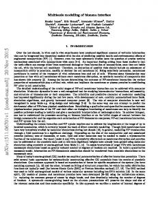
In a recent study by Cornelissen [75] friction between carbon tows were measured with the help of a capstan-type test setup. One of the objectives of this test was to determine the effects of parallel and perpendicular inter-tow orientations on tow friction. The tests were carried out on pre-tensioned 3k and 12k tow sizes (Figure 2-19). The parallel orientation gave high friction coefficients which were about double the magnitude obtained in the perpendicular orientation (Figure 2-19(e)). This is because; when the fibres are parallel, the propensity of the fibres to tangle, migrate and embed increases which increases the friction force. The main assumption of this study was that the friction behaviour of a tow on a 0o/90o weave was considered equivalent to the friction between perpendicular tows.
(a)
(b)
32
(c)
(d)
33
(e) Figure 2-19. Test setup for (a) tow on smooth metal surface, (b) tow on rough metal surface, (c) parallel tow orientation, (d) perpendicular tow orientation, and (e) Coefficient of friction for carbon fibres in all these test configurations [75] Ersoy et al. [76] developed a test setup to study the frictional interactions during composites manufacturing which are encountered due to uneven thermal expansions of the tooling and composite part. The study measured the friction between the tool and a ply and between the plies. A schematic is shown in Figure 2-20 which illustrates the pulling of a unidirectional ply against the surface of another ply. The surfaces of the plies were heated with stainless steel heaters and a temperature controller was used to record the cure temperature. An instron is employed to measure the pulling force and displacement and the inter-ply friction coefficient was finally calculated using Amontons’ law.
34
Figure 2-20. Schematic for pull-out test [76] Dong and Sun [77] investigated the yarn pull-out in Kevlar fibres (Figure 2-21). A fabric specimen was clamped and a yarn was pulled mid-way between the clamps. The force and displacement of the yarn was measured with the help of an instron cross-head. A two-dimensional FE model was developed to simulate single yarn pull-out procedure. The model predicted the maximum pull-out force which was comparable with the experiments.
35
(a)
(b) Figure 2-21. (a) Fibre pull-out test setups (b) Load versus displacement trace [77] To summarise, a number of friction tests was adopted to find out fibre friction. The capstan type test set up was common in order to study the effects of tow orientation (perpendicular or parallel) on fibre friction. However, the friction anisotropy was not studied for the orientations or angles lying within these extremities – parallel and 36
perpendicular which are widely encountered during the draping process. In addition, there were no studies to investigate the effect of filament friction on overall tow friction. 2.4
Analytical models of stick-slip friction This section reviews the models developed to study the stick-slip friction
behaviour. Early researchers investigated the stick-slip friction behaviour with the help of a single degree of freedom system (SDOF) [78-94]. Korycki [78] developed a mathematical model of stick-slip friction for an SDOF system which depended on the slip speed characteristics (Figure 2-22 (a)). The differential equation of motion of mass m when subjected to a constant force, F was solved to find out the stick-slip nature of the displacement, x.
Figure 2-22. Friction force vs slip speed model [78] Pratt and Williams [79] analysed a two mass, two degree-of-freedom system excited by harmonic forces and proposed a solution procedure for a steady state response of a two mass system. A non-dimensional measure of energy dissipation due to Coulomb friction was developed which predicted the damping force for maximum disspation. An SDOF model of a violin string was studied by Leine et al. [84] who developed a switch model consisting of a set of ordinary differential equations which can be integrated with any standard solver. He used this model to find out torsional vibrations of a violin string with radius r, torsional stiffness kt, axial stiffness k, polar moment of inertia J, and a bow moving with a constant velocity, vdr over the string. The friction force induced lateral displacement x and rotation φ (Figure 2-23). The study concluded that the 37
frequency ratio of the torsional vibrations to the lateral vibrations was proportional to the diameter of the string (2r) ((c)).
Figure 2-23. Voilin string SDOF model [84] Sakamoto [80] developed a pin-on-flat apparatus in order to model the friction force – velocity relationship. Figure 2-24 (a-d) show the steps of stick-slip motion of a mass with the help of an SDOF system and corresponding stick-slip behaviour. A steady stick slip trace was observed from the measured displacement and acceleration of the sliding element. A sliding mass (m) was supported with the help of a spring (stiffness, k) and a dashpot (damping coefficient, c) on a flat surface (S) which was subjected to a linear speed. Figure 2-24 (a) represents the equilibrium position of the mass where both the friction force and spring deflection are equal to zero. When the surface was applied a velocity and the spring force did not exceed the friction between the mass and the surface, both moved together with zero relative velocity, called as the “sticking time” (graphically in Figure 2-24 (d)). When the spring force exceeded the static friction force, the body began to move/slip abruptly, thus slip initiation took place (Figure 2-24 (d)). Once, the slip began, a dynamic motion was carried out till a steady state was reached between the friction force and spring force.
38
Figure 2-24 (a-d) Schematic for basics of stick-slip phenomenon Billkay and Analgan [88] developed a mathematical stick-slip analysis model to prevent stick-slip motion of the slideways that would affect normal running of the machine tool by providing proper dampers. In brief, the models used the concept of SDOF systems to simulate the stick-slip friction behaviour. The friction behaviour of carbon fibres can be modelled utilising similar concepts at filament- and tow-level. 2.5
Review on mechanical tests of carbon fibres The earliest fibre compression test was done by Kawabata [95] who developed a
test rig in order to measure the transverse modulus of fibres of diameter ranging from 5-15 µm. The advanced high-performance fibres such as aramid, carbon were studied in the test. The carbon and ceramic fibres exhibited brittle behaviour during compression.
39
(a)
(b)
Figure 2-25. (a) Experimental setup (b) Diametric compression of a single fibre [95] A single fibre was compressed with the help of an anvil (Figure 2-25 (a)). The anvil was driven electro-magnetically with an ultimate load of 50 N. Miyagawa et al. [96, 97] used the technique of Raman Spectroscopy to measure the transverse modulus of carbon fibres in carbon fibre reinforced polymer (CFRP) specimens. Tensile specimens of CFRP (which was composed of epoxy resin #2500 and T300 carbon fibre) were prepared and a thin film of lead oxide was deposited by resistance-heating physical vapour deposition method to measure strains in carbon fibres and matrix phases separately. Figure 2-26(a) shows the schematic of strain measurements.
40
(a)
(b) Figure 2-26. (a) Experimental setup (b) 2D plane strain model [97] Raman spectroscopy was used to measure strains in individual fibres and in the resin matrix of a CFRP specimen. The transverse strains were then analysed by finite element methods. The transverse modulus of the fibres was determined by changing the modulus in numerical models to fit the experimental result of strains obtained from Raman spectroscopy. A two-dimensional FE model was developed for the purpose and the transverse strains were predicted on a carbon fibre and epoxy matrix (Figure 2-26 (b)). The mechanical properties of carbon fibres and epoxy matrix used in the numerical model are listed in Table 2-1.
41
Table 2-1: Mechanical properties of carbon fibres and epoxy matrix
Materials
E1 (GPa)
Epoxy
3.00
E2 (GPa)
v12
v22
0.300
G12 (GPa)
G22 (GPa)
1.15
resin(#2500) Carbon
230
8.00
0.256
0.300
27.3
3.08
fibre(T300)
Nano-indentation tests were also done to find out the transverse modulus of CFRP. The transverse modulus which was obtained from different techniques was compared as shown in Figure 2-27. It shows that the elastic transverse modulus lied between 5-14 GPa except for 3D FEM analysis which was apparently because of the Poisson’s effect of the fibres and the mesh size of the solid tetrahedral elements.
Figure 2-27. Comparison of transverse elastic modulus from different models [97] Standardised tensile test (BS ISO 11566:1996) is available where a single filament specimen can be prepared to measure the tensile modulus in a tensile testing machine, 42
instron [98, 99]. The specimen is to be made of a thin cardboard frame of dimensions as in Figure 2-28(a). Then, it requires to be clamped between two cross-head grips such that the loading axis is parallel to the longitudinal axis of the fibre. At the onset of loading, the two lateral ends of the frame in midway are to be cut or burnt so that the load will only be borne by the fibre. A linear speed of 5-10 mm/min is to be applied to the instron cross-head. The load extension curve can then be obtained from the test and the initial slope will reflect the longitudinal modulus of the specimen. The magnitude of linear speed of instron used in the friction tests (discussed in Chapter 3) was taken from this standardized test principle.
(a)
(b)
Figure 2-28. (a) Dimensions (mm) of the cardboard frame (b) Specimen mounting [98] 2.6
Discussion Limited works were carried out to include the filament-level phenomena such as
filament migration, filament count and filament friction on the overall compaction models of fabric or tows [16-18, 22, 25, 28]. Most of them were numerical (FE based) models both at filament- and tow- level. Filaments were assumed straight and filament friction was neglected in these models because of computational complexity. The existing filament friction tests were carried out either between two perpendicular filaments or
43
between two twisted filaments. So it lacks the information of filament friction when the filaments are parallel – which is common in case of a tow. Compaction tests at the tow and fabric level which are available in the literature include effects of tow spreading, twist and fibre diameter on the compaction behaviour [4-7, 10, 47-52, 100-121]. But none established a complete relationship of the compacted thickness as a function of all the important parameters such as tow size, twist, pre-tension and compaction pressure. The existing numerical models of compaction of fibre bundles considered a maximum of 450 filaments [16-18, 21-31] as the computational cost increased exponentially with filament count. As a result, the models were inconclusive to predict the realistic compaction of fibre bundles and to study the effects of filament-level features such as filament slippage, filament arrangement, filament count on the compaction behaviour. The following section addresses what strategies are followed to overcome these shortcomings. The corresponding chapters are included in the parentheses for ease of understanding the layout of the thesis. 2.7
Concluding remarks The need for investigating friction anisotropy in terms of inter-tow angle at tow-
level is highlighted in [53-75] such that accurate numerical prediction of draping process can be undertaken. The present study carries out a detailed experimental study on the tow friction for a wide range of inter-tow angles (0o to 90o). The experimentally-obtained tow friction coefficients can be used to update the tow friction behaviour with the change in tow orientation while simulating a draping process (Chapter 3). The filaments within a tow can slip relative to each other which suggest that there could be an effect of filament friction on tow friction, that is, the tow friction coefficient might be an apparent coefficient. In addition, to accurately model the compaction of tows or fabrics at filament-level, inter-filament friction coefficients are required. A numerical study is carried out to find the inter-filament friction within a large fibre bundle (say, 12k tow) and study its effect on overall tow friction (Chapter 4). As discussed in Section 2.6 a complete relationship of compacted thickness of tow as a function of the parameters such as tow size, twist, pre-tension and compaction 44
pressure is missing. Chapter 5 is dedicated to derive such an empirical relation which can be used by composite manufacturer to predict the compacted thickness of a tow or a ply beforehand. Finally, efficient methodologies are required to be adopted which can predict the compaction of large fibre bundles and consider inter-fibre contacts. Chapters 6-8 deals with such methodologies and the methods are improvised with newer engineered techniques. The proposed models consider high filament count (12k), filament friction and filament distribution and are computationally efficient.
45
Chapter 3 Friction tests on carbon tows 3.1
Introduction The composites industry is interested in automated forming processes for the
manufacture of parts made of advanced polymer matrix composites (PMCs) in conjunction with high fidelity simulation tools. Discontinuous fibre systems such as conventional sheet moulding compounds (SMCs) and advanced moulding compounds such as HexMC [122], are easily formed into complex shapes. On the other hand, continuous fibre systems in the form of prepregs or dry fabrics are prone to wrinkling and intra-ply tow slippage during automated drape-forming processes. Therefore, careful process planning is necessary with the help of the ‘process simulation’ (- this refers to composite manufacturing and forming process models) tools. Friction plays a significant role during the processing (i.e. draping, weaving, braiding) of prepregs as well as dry fabrics due to the interactions which occur at different scales of a fibre preform – i) at macro-scale between ply/ply and tool/ply; ii) at meso-scale between tow/tow within a ply and iii) at micro-scale between fibre/fibre within a tow [16, 17, 24, 29, 45, 123-135]. Macro-scale inter-ply or tool-ply interactions may lead to the formation of wrinkles [127, 130, 131, 136-140]. Meso-scale interactions are encountered at the tow-level both in the case of draping and moulding techniques. During draping, sharp double curvatures are formed where the inter-tow angle within a ply changes (say, from 90° to as low as 20°) with the advancement of the drape tool [136, 141-145]. This change in the inter-tow angle may affect the frictional behaviour between the tows. In order to accurately predict the draping process the frictional behaviour needs to be updated with the change in the inter-tow angle [25, 32, 135, 146-149]. In case of moulding techniques, during the compaction stage the inter-tow orientations can be of 46
any value (between 0°– 90°) depending on the ply orientations as well as the state of inplane shear. This requires an understanding of the influence of the inter-tow orientation for an entire range of values (0°– 90°) on the fibre friction behaviour. Many of the past studies ignored this influence and assumed that the coefficient of friction is independent of the tow orientation [18, 19, 22]. A recent study by Cornellissen et al. [75] demonstrated the difference in the effects of parallel (0°) and perpendicular (90°) intertow orientations on tow friction due to the occurrence of inter-fibre phenomena such as fibre migration and entanglement at the lower inter-tow angle. This chapter presents an experimental investigation of coefficient of friction as a function of inter-tow angle, tow size and contact pressure. A capstan-based test rig was developed which simulates the inter-tow friction behaviour during fabric processing. 3.2
Brief review on fibre friction A brief review of fibre friction is presented in this section for the ease of
understanding. Studies of friction in textiles began in 1940s on natural fibres such as cotton and wool [47, 54, 55]. They were concerned with the processing of fibres and subsequent comfort of apparel. The fibre friction tests are broadly classified into four types – fibre-twist method, capstan-type test setup, tool/ply or ply/ply friction tests using friction contactor, and fibre pull-out tests. These tests were developed on the basis of Amontons’ law of friction (Equation 2-7). Gralen and Olofsson [54] developed a fibre-twist method to measure the inter-fibre friction. In this setup dead weights were applied at one end of the fibres and the other end was pulled till slippage occurred. The coefficient of friction was calculated at the onset of slippage. In another study by Roselman and Tabor [66], a capstan setup was developed where a fibre was pulled over a cylindrical counterface and the friction coefficient was calculated using the belt friction equation (Equation 2-8). In addition to these, inter-ply friction and fibre pull-out tests were common which used Amontons’ law of friction. Potluri and Atkinson [150] devised a friction test setup in order to measure the coefficient of friction between a fabric ply and a mould surface. The apparatus employed a robotic arm with a metallic friction contactor (in this case, the mould surface) which applied a normal force on the fabric ply. A dead weight was placed 47
on the ply and the arm displaced the contactor slowly away from the dead weight to avoid any fabric buckling. The friction coefficient was then evaluated by dividing the friction force by the normal force from the contactor. The study was further extended to measure the inter-ply friction forces by wrapping a fabric ply on the contactor and similar tests were carried out to determine the friction between the top ply (that is, the fabric strip attached to the contactor) and the bottom ply (that is, the fabric panel). Other studies involved yarn pull-out tests on a Kevlar fabric strip which was clamped between two grips and the strip was without any pre-tension in a direction transverse to the direction of pull-out [77]. A yarn was, then, pulled from midway between the grips and the friction of Kevlar yarn was estimated from the pull-out force. They concluded that the pull-out force oscillated with the displacement when the pulled yarn passed every cross-yarns (yarns which were perpendicular to the pulling direction) in the fabric. The study in this chapter was focussed to estimate the dependence of the coefficient of friction on the inter-tow angles (that is, inter-ply tow orientations). Effects of parameters such as load (which directly relates to the contact pressure), and tow size (filament count within a tow) were subsequently studied. 3.3
Experimental methodology This section discusses the experimental rig, material used, and experimental
procedure which was used to conduct the fibre friction tests. 3.3.1 Experimental rig The test rig employed three stationary pulleys as shown in Figure 3-1 (a). The figure was captured during the tow friction test on bare pulleys. An instron tensile tester (Model, 5564; load capacity = 1kN; accuracy = ±0.04 N) was used for the purpose. Figure 3-1 (b) shows the three angles of wrap or contact angle () formed by the passing tow with the pulleys (C1, C2 and C3) – (i) 2=2.87 radians (=164.4o between C1 and C2), (ii) 2=3.57 radians (=204.5o between C1 and C3), and (iii) 2=4.92 radians (=281.9o between C2 and C3). Each pulley has an inner diameter of 38 mm and width of about 18 mm. The rig was clamped to a stand such that the length of the passing tow from instron cross-head to the first pulley, in any of the three combinations, was parallel to the length 48
from which the dead weight was suspended. A linear cross-head speed of 10 mm/min was used for all the tests.
(a)
49
(b) Figure 3-1. (a) Experimental rig (b) Three angles of wrap 3.3.2 Material used Carbon tows were used to characterise the fibre friction. The manufacturer’s specification (Toray Carbon Fibres America, Inc) of the tow was T700SC-12000-50C where T700S denotes a tensile strength of 711 ksi or 4.9 GPa, C denotes that the fibres were never twisted, 12000 is the tow size (i.e. filament count), and 50C is the sizing specification (where 5 represents the system compatibility with the resins, 0 denotes that the surface is treated for better adhesion with resins, C denotes the amount of sizing added to the fibres for better handling and weaving) [151].
3.3.3 Experimental procedure Tows of 450 mm length were glued to stiff papers at both ends. The paper at one end was attached to the instron cross head while a dead weight was suspended from the paper at the other end using a piece of thread and a clip (Figure 3-1 (a)). The magnitude of dead weights (30 cN – 60 cN; 1 cN = 0.01N) which were chosen for a 12k tow is 50
based on the works of Roselman and Tabor [66] where they considered 1 mg pre-tension for a single carbon filament. The applied load on the tow was, thus, effectively the sum of dead weight and an additional constant load of 2 cN (that is, the combined weight of thread, clip and stiff paper). This applied load and the output force from the instron was then used in Equation 2-8 to determine the coefficient of friction at a particular angle of wrap. The inter-tow angle being the important parameter in this study, care was given to prepare the tow specimens which would reflect this angle. The term ‘inter-tow’ angle, in this case, represents the angle subtended by the passing tow (which was attached to the instron cross-head) with another tow pasted on the pulley. Thus, friction would be encountered between the passing tow and the pasted tow pasted at a particular angle. The methodology to prepare the specimens is as follows – tow samples of required lengths were pasted on one side of a double-sided adhesive tape at a desired angle (for each inter-tow angle of 90°, 75°, 65°, 45°, 35°, 25°, 15°, 10°, 5°, 0°). The length of the pasted tow was equal to the circumferential length of the pulleys such that during the fibre-onfibre friction test no part of the passing tow came in contact with the bare pulley (i.e. no effect of tow-pulley friction on tow-tow friction). The width of the adhesive tape was kept similar as the width of the pulley and the length was enough to wrap the pulley surface. The other side of the tape was, then, peeled off to stick the pasted tow on the surface of the pulley (Figure 3-2 (a, b)). So, the pasted tow angle represented the intertow angle with the direction of the passing tow. While conducting the tests for 0° inter-tow angle (that is, when the fibres are parallel) the fibres of the passing tow were found to pull off the fibres from the pasted tow on the pulleys which showed sharp peaks of friction values in the results. A special modification was done only for this inter-tow angle by attaching tapes to restrain the free ends of the wrapped tow from movement.
51
(a)
(b)
Figure 3-2. (a) Schematic of inter-tow angle (b) Pasted tow at inter-tow angle of 45° To investigate the effect of tow size 12k tows were split manually in order to produce tow specimens of different filament counts. The filament count for the split tows were then estimated by weighing them in an electronic balance. Four tow sizes were considered for the study. That is, a full 12k tow was split thrice to get tows of about 6k, 3k and 1.5k filament counts. The tests were run both on bare and tow-pasted pulleys for ten trials and standard error bars are plotted with a variation of 1.96
n
(where, is the standard deviation
for a set of n 10 trials) across the mean for 95% confidence level. The effect of direction of instron cross-head movement on the coefficient of friction was investigated for one set of angle of wrap (2.87 rad). Influence of test repetitions in the contact zone was also investigated.
3.4
Results and discussion This section discusses the influence of parameters such as inter-tow angle, tow size,
load and angle of wrap on the tow friction and understanding the experimentally obtained signals in the frequency domain using spectral analysis tools. 52
3.4.1 Determination of coefficient of friction The final tension force versus displacement for 32 cN load on 12k tow specimens for all ten trials is shown in Figure 3-3 which includes details of all the signals. A Matlab code was developed to post-process the signals and compute an average force for a displacement of 10 mm (loading time = 1 min) (Appendix A.1). The program used a ‘ginput’ command to select a window from the signal and then calculated the mean tension force. This final tension force was then incorporated in the belt friction equation to determine the coefficient of friction for an applied load and an angle of wrap (Equation 2-8). This equation assumes a uniformly distributed normal pressure along the arc of contact (wrap).
Figure 3-3. Friction of 12k tow with bare pulley for an applied tension of 32 cN 3.4.2 Effects of inter-tow angle Figure 3-4 shows the variation of coefficient of friction with change in the inter-tow angles for different tow sizes. A horizontal line denoting the coefficient of friction (in this case, 0.23) between the tow and the bare pulley surface is also shown. The graph shows that the fibre/pulley friction and the fibre/fibre friction at an inter-tow angle of 90° are close as observed from the tests. A reduction of inter-tow angle from 90° to 45° reduces 53
the friction coefficient marginally by 10%, however, a further reduction to 0° (that is, when the fibres are parallel) rises the friction sharply to a value of 0.45 which is about double of the friction at 90° inter-tow angle. The experimental results from Cornelissen’s [75] study for 0° and 90° inter-tow angles also compare well with the present trend (Figure 3-4). A detailed explanation of the physical phenomena occurring in this case is provided as follows. When the passing and the pasted tows are parallel (that is, for 0° inter-tow angle) the friction coefficient is significantly higher which is due to the trapping or bedding of fibres of the passing tow on the gaps of the pasted tow. Some of the pasted fibres were seen to be entangled with the passing tow and were pulled out from the top layer of the pasted tow against their cohesive bonding as the bottom layers were rigidly glued to the pulley surface. This phenomenon increased the friction at 0°. As the inter-tow angle increases the trapping of fibres reduces which lowers the frictional force. For an increase in inter-tow angle from 0° to 90°, the length of the fibres on the pasted tow shortened from along the pulley circumference to across the pulley width. This shortening of fibre length (i) reduced the bearing support of the pasted tow on the pulley, (ii) changed the direction of traction force from along the fibres to across the fibres of the pasted tow, and (iii) increased the fraction of length of an individual fibre, and the number of fibres in contact with the passing tow. It is to be noted that as the top fibres on the pasted tow were not glued to the pulley surface, inter-fibre cohesion was the only restraining force. So, the fibres at the top layer of the pasted tow displaced more for higher inter-tow angles due to the first and second reasons described above. This meant that the inter-fibre cohesive forces within the layers of the pasted tow had to be mobilised first before any slipping of the passing tow occurred. However, from 45° onwards, the combined effect of all these factors was to increase the friction forces slightly with an increase in the inter-tow angle which is evident from a careful observation of the trend of the friction behaviour.
54
Figure 3-4. Effects of inter-tow angle on tow friction 3.4.3 Effects of tow size Figure 3-5 compares the coefficients of friction between the passing tow and the bare pulley, and between the passing tow and the pasted tow for same angle of wrap (in this case, 2.87 rad) and same applied load (in this case, 52 cN). Tow sizes of 6k, 3k and 1.5k are approximate as they were split manually, hence the data points are not at fixed locations along the abscissa. It can be seen from the plot, when the tow size was reduced to 1/10th of the maximum filament count (in this case, 12000), the fibre/pulley friction and the fibre/fibre friction at 90° inter-tow angle were decreased by 12% and 10% respectively, indicating a weak effect of tow size on fibre friction.
55
Figure 3-5. Coefficients of friction for different tow sizes Effects of tow size for different inter-tow angles at the same angle of wrap of 2.87 rad and a load of 52 cN are shown in another figure (Figure 3-6). This figure is an alternate representation of Figure 3-4 in order to investigate the influence of tow size on frictional behaviour. The fibre/fibre friction at 0° inter-tow angle shows a weak increasing trend with reduction of tow size (that is, an increase by 6% when the tow size is reduced to 1/10th of maximum count). For the same magnitude of applied tension, perfibre load increases when the tow size is reduced. This increases the normal load which is proportional to the per-fibre load and as a result, the chances of bedding of fibres are higher. Another cause is the increase in percent of fibres of the passing tow which gets embedded in the pasted tow when the tow size is reduced. That is for the same value of applied tension when the tow size is reduced more number of fibres tend to embed in the gaps of the pasted tow. Rest of the plots for fibre/fibre friction at the inter-tow angles (from 5° to 90°) show that the effect is independent of the tow size. The mean and standard deviation of the friction coefficients at different inter-tow angles are presented (Table 3-1) for convenience.
56
Figure 3-6. Coefficients of friction versus tow size for different inter-tow angles
57
Table 3-1: Mean and standard deviations of the friction coefficients of Figure 3-6 Inter-tow
12k carbon tow
6k carbon tow
3k carbon tow
1.5k carbon tow
Mean
S.D.
Mean
S.D.
Mean
S.D.
Mean
S.D.
90o
0.23
0.007
0.21
0.005
0.21
0.006
0.19
0.005
75o
0.21
0.004
0.195
0.004
0.195
0.004
0.19
0.003
65o
0.204
0.005
0.202
0.005
0.194
0.004
0.189
0.008
45o
0.198
0.004
0.203
0.005
0.198
0.004
0.203
0.008
35o
0.265
0.016
0.230
0.005
0.246
0.017
0.232
0.024
25o
0.24
0.01
0.235
0.008
0.216
0.005
0.240
0.014
15o
0.264
0.007
0.285
0.011
0.26
0.01
0.272
0.005
10o
0.285
0.002
0.287
0.003
0.274
0.004
0.286
0.002
5o
0.315
0.003
0.319
0.002
0.31
0.003
0.322
0.004
0o
0.429
0.008
0.438
0.014
0.442
0.013
0.457
0.021
angles
3.4.4 Effects of loading and angle of wrap Studies concerning the effects of direction of cross-head movement exist in literature which investigated the scale effects of wool fibres [68, 69]. A range of loads (32 cN – 82 cN) was chosen to study the influence of load and loading direction in carbon fibre friction. Figure 3-7 shows the plot for fibre friction versus load in different loading directions for one set of angle of wrap (in this case, 2.87 rad). The graph shows nearly steady value of coefficient of friction with increase in load at same angle of wrap which satisfies the belt friction equation (Equation 2-8). When the instron cross head ascends it pulls the fibres and overcomes the suspended dead weight, whereas, when the cross-head descends it is the load applied to the fibres that pulls them down. The graph reflects a decrease of friction coefficient by 19% when the load is increased from 32 cN to 62 cN during the cross-head upward 58
movement. But a further increase in the load shows a steady trend in the friction coefficient. On the other hand, when the instron cross-head descends, if the magnitude of the suspended load is not sufficient then chances of buckling and slippage may occur that reduces the apparent coefficient of friction as observed for the load range of 32 cN – 52 cN. Hence to carry out tests with reverse loading, sufficient load is to be applied to avoid such phenomena. Whereas, at higher loads (that is, above 52 cN) these phenomena were not observed and the friction shows a steady trend independent of load and the loading direction. Therefore, unlike the wool fibres, the carbon fibres do not have scales on their surfaces and show similar friction behaviour beyond a particular range of load. This can also be observed from the SEM images of the surface of the carbon fibre (Figure 3-10 (b)).
Figure 3-7. Coefficients of friction for different loading directions Figure 3-8 shows the effect of loading on friction of 12k tow at 2.87 rad angle of wrap and for different inter-tow angles. All the plots for different inter-tow angles show nearly steady trend indicating a weak influence of load whereas, there is a high rise when the passing tow is parallel to the tow wrapped on the pulley. This high rise in friction coefficient was due to jamming, bedding, tangling of fibres as discussed earlier. 59
Figure 3-8. Coefficients of friction on different loads for 12k tow Figure 3-9 (a, b) plot the logarithms of frictional output-input load ratio for 12k carbon tow against angle of wrap for different loading on unwrapped pulley and fibre wrapped pulley. Based on the belt friction equation (Equation 2-8), the slope of logarithm of T2/T1 versus the contact angle is the coefficient of friction. A reduction of the slope is observed in Figure 3-9 (a) that is, a reduction in the coefficient of friction by 9% when the angle of wrap was increased from 3.57 rad to 4.92 rad. The trend shows an increase of this load ratio with the angle of wrap but is not directly proportional to angle of wrap which suggests an improvement in belt friction equation may be required for this purpose. In case of tow-pasted pulley the slope (i.e. the friction coefficient) of the plot is fairly linear with change in applied load (Figure 3-9 (b)).
60
(a)
(b) Figure 3-9. Output-input force ratio vs angle of wrap for (a) bare, and (b) tow-pasted pulley at 90° inter-tow angle 61
3.4.5 Influence of test repetitions in the contact zone Surface characteristics tests were conducted by carrying out repeated tests on the same and different contact zones. Figure 3-10 (a) shows the friction behaviour of a 12k tow when same and different area(s) of contact are considered for a repeatability test with same load (42 cN) and an inter-tow angle of 90°. This concludes that with increase in the number of tests that is, increasing the number of times the tow is rubbed over tow-pasted pulley, the interface becomes smoother which increases the chance of slippage and slightly decrease the friction (in this case, a friction coefficient reduction of 13% from test number 1 to test number 10). However, for the case of different zones of contact such decreasing trend was not observed. An SEM image of a T700 carbon fibre was provided which shows the virgin surface with unevenly distributed asperities (Figure 3-10 (b)).
(a)
62
(b) Figure 3-10. (a) Surface characteristics tests on 12k tow (b) SEM image of a T700 carbon fibre 3.4.6 Spectral analyses of experimental signals The experimental signals were further analysed to find out the stick-slip frequency of the friction behaviour. This information was later used in the following chapter (Chapter 4) while modelling inter-filament friction in order to reproduce the stick-slip friction behaviour. The test data were not uniformly spaced in time domain (maximum data rate was 20 Hz). The load cell is built in such a way that it stores data when it receives the raw signal throughout the test [152]. As a result, during the test, once slippage has occurred this data rate reduces which creates the non-uniformity in sampling rate. So non-unform spectral analysing techniques were used for the purpose. In this case, three techniques were employed – i) Lomb Scargle periodogram (LSP), ii) Non-uniform discrete Fourier transform, and iii) Finite Fourier expansion of signals. Lomb and Scargle [153-155] proposed a spectral analysis algorithm to investigate the frequencies of an unevenly spaced data over a time period. The periodogram is expressed in Equation 3-1 and a Matlab function (lombscargle.m) for LSP method was used to carry out the frequency analysis of the signals.
63
Equation 3-1
d (ti ) A cos(2 fti ) B sin(2 fti ) ni
where d (ti ) is the sample over time ti , A, B are the cosine and sine amplitudes of the sinusoid, f is the frequency to be estimated, ni represents noise at time ti , and was chosen to make sine and cosine model functions orthogonal on the discretely sampled time intervals. The parameters of Equation 3-1 can be obtained through the least square method [156]. The algorithm is available as a Matlab built-in function and has been used in this context.
Figure 3-11. Signals of friction test for 30 gms load and 2.87 rad angle of wrap at an inter-tow angle of 90o The experimental signal shown in Figure 3-11 has been analysed using the LSP method and the power-frequency plot is drawn (Figure 3-12). The values of in the figure denote how significant a peak is in the spectrum where is the probability that a value of power (PN ()) at a particular frequency () will lie between two positive values [156].
64
Figure 3-12. Lomb scargle periodogram of signals The second spectral analysing technique used is the non-uniform discrete Fourier Transform (NDFT), defined in Equation 3-2 [157]. N 1
Equation 3-2 P(m) pn e
j
2 mtn T
0
where the samples P(m) are taken at m multiples of a quantity which corresponds to 2 T (that is, the frequency (rad/s)), T is the range of the samples, and N is the sample size.
A Matlab code was written to implement Equation 3-2 and the frequency plot was developed for each test trial (Appendix A.2). Figure 3-13 illustrates the frequency diagram using the NDFT technique.
65
Figure 3-13. Non uniform discrete fourier transform of signals In the third technique, which is the Finite Fourier expansion of signals another Matlab code was written which represented the sampled data in the form of the following equation (Equation 3-3) (Appendix A.3) N 1
Equation 3-3
f ( x) a0 an sin(nx) bn cos(nx) n 1
where f ( x) is the sampled data, an , bn are the coefficients and N is the sample size. The coefficients ( a0 , an , bn ) are evaluated using the trapezoidal rule of integration and the normalised spectral power is plotted against the frequency. The frequency range ( f range ) was obtained using Equation 3-4. Figure 3-14 shows the plot of spectral power and frequency for the experimental signal (Figure 3-11). Equation 3-4
f range 0 : finterv : ( N 1) finterv
where T is the total time period, f interv
1 ; is the sampling interval; N
T . In this case, N = 1293, T =180 sec, = 0.1393 sec. N 1
66
Figure 3-14. Finite fourier expansion of signals Table 3-2: Effects of inter-tow angle on frequencies of experimental signals Inter-tow angle
Significant frequencies (Hz)
0o
4.01
5o
3.99, 4.02
10o
3.99
15o
4.1
25o
3.995, 4.006
35o
3.983, 3.995
45o
3.998, 4.5
65o
3.499, 4.008
75o
4.002
90o
3.99, 4.003 67
Table 3-3: Effects of tow size on frequencies of experimental signals Tow size
Significant frequencies (Hz)
1.5k
3.45, 4.5
3k
3.49, 4.49
6k
3.52, 4.3
12k
3.98, 3.99
Table 3-4: Effects of loads (cN) on frequencies of experimental signals Load (cN)
Significant frequency (Hz)
32
3.992
42
3.985
52
3.982, 3.995
62
3.975, 3.984
Table 3-5: Effects of angle of wrap (rad) on frequencies of experimental signals Angle of wrap (rad)
Significant frequencies (Hz)
2.87
3.982, 3.995
3.57
3.97, 4, 4.01
4.92
3.994, 4.001
68
Using the spectral analysing techniques (that is, LSP, NDFT and Finite Fourier Expansion of unevenly spaced data) the frequency plots (Figure 3-12, Figure 3-13 and Figure 3-14) show the dominant frequencies close to 4 Hz for 12k tow friction tests. The actual magnitudes of significant frequencies are tabulated to study the effects of inter-tow angle (Table 3-2), tow size (Table 3-3), load (Table 3-4) and angle of wrap (Table 3-5). The sampling rate during the friction tests was 20 Hz and Equation 3-4 suggests that the frequency would lie within 0-8 Hz. The experimental signals are typically of stick-slip pattern so with a loading rate of 10 mm/min and a frequency of 4 Hz it can be concluded that a displacement of 41.67 µm occurs which is a part of the wavelength for the maximum slippage. 3.5
Conclusions Inter-tow friction was determined by using a capstan-type experimental rig. The rig
consisted of stationary pulleys and suitable combination of any two pulleys gave rise to the angles of wrap which were used during the tests. Parametric studies were carried out to study the effects of inter-tow angles, tow size, load and angle of wrap on tow friction. The study on the effects of inter-tow angle estimates the frictional behaviour between the plies during the drape-forming processes. The main highlight of this chapter is that the inter-tow angle has a dominant role in the tow friction. The friction coefficient for 0° inter-tow angle reaches to a magnitude (μ = 0.42) which is about double the magnitude (μ=0.23) at the inter-tow angle of 90°. At lower inter-tow angles the effects of phenomena such as bedding of fibres, fibre migration and entanglement are prominent, which increases the coefficient of friction. Table 3-6, presented below, reports the friction coefficients of 12k carbon tow at a range of inter-tow angle. This information of friction coefficient would be useful for the drape simulation tools which require prior knowledge of tow friction coefficients at a particular inter-tow angle in order to predict the draping process accurately.
69
Table 3-6: Friction coefficients at a range of inter-tow angles for 12k carbon tow
angles
Mean Friction coefficient at different inter-tow angle
90o
0.23
75o
0.22
65o
0.21
45o
0.20
35o
0.26
25o
0.24
15o
0.27
10o
0.28
5o
0.32
0o
0.42
Inter-tow
The tow size had a weak effect on the friction coefficient. It was observed that the friction coefficient reduced by 10% when the tow size is lowered by 1/10th (that is, from 12000 to 1500 filaments). This occurs both in the case of fibre/pulley friction and friction between the passing tow and pasted tow on the pulley surface at an inter-tow angle of 90°. However, when the effect of tow size was studied for 0° inter-tow angle, there is a slight increase in the friction coefficient which is due to the effects of tangling of fibres from the passing tow on the pasted tow.
70
Chapter 4 Numerical model of fibre friction 4.1
Introduction The compaction model of a tow at filament scale requires magnitude of filament
friction to consider the inter-filament interactions. In order to predict the compaction process the magnitude of filament friction coefficient needs to be carefully estimated. A real tow consists of thousands of filaments (in this case, 12k filaments in a carbon tow). Hence it is difficult to measure the inter-filament friction within a real tow experimentally and satisfactory literature is not available to determine intra-tow inter-filament friction. An alternative approach is to estimate the magnitude of filament friction using finite element technique. This chapter develops numerical models to estimate the absolute magnitude of filament friction and a range of friction coefficient within which interfilament slippage begins within a tow. The results obtained from the experimentallydetermined tow friction (Chapter 3) were considered as a benchmark for determining inter-filament friction. The current research attempts to model the stick-slip friction behaviour of carbon tows observed in Chapter 3. Past works [78-94] demonstrated the use of single degree of freedom (SDOF) to find out the stick-slip displacement of a mass where the mass was attached to a free spring. The spring was applied a pull force and the mass was subjected to a normal pressure. In the friction experiments (in the case of a tow passing over the bare pulleys), the length of the tow resting on the pulley can be assumed to be an equivalent mass on a rigid surface (pulley). The free length of the tow (which is not in contact with the pulley) can replace a spring attached to the mass. The pull force in this case is a displacement applied by the testing machine (Instron) to the free end of the tow. The solution to such a differential problem will provide the stick-slip displacement of the mass. 71
During friction tests, the experimental signal of tow friction represents stick-slip behaviour of the final tension force (obtained from the instron) with the loading time (Figure 4-1). The ordinate of the figure is rationalised per unit applied tension force in order to compare the friction behaviour with that of filament-level models. The figure suggests that an idealised representation (that is, an ideal stick-slip behaviour) of the signal was required to model the frictional behaviour as the stick-slip amplitude was not uniform. In order to model this stick-slip behaviour the parameters such as static and dynamic friction coefficients, amplitude and frequency were chosen at specific time points. The strategy used to model the frictional behaviour is detailed in the next paragraph.
Figure 4-1. Experimental signal of friction behaviour of a 12k tow A user friction algorithm was proposed and implemented in Abaqus with the help of a user subroutine (UFRIC) which was written in Fortran. The friction coefficients (µs0, µsand µk), the relative amplitude of friction (A) and the frequency (f in Hz) were selected at specific time points for the numerical analysis (Figure 4-1). Sensitivity studies of the friction coefficients were carried out to investigate their effects on the relative amplitude and the frequency of the response obtained with the help of the user subroutine. Subsequently, an optimum set of coefficients was obtained from the sensitivity studies which reflected the overall tow friction behaviour. The study is then extended to estimate the magnitude of filament friction coefficients. 72
The following section discusses a brief review on filament friction and then continues with the modelling approach, the results and discussion. 4.2
Brief review on filament friction Most of the process simulations which attempted to predict the manufacturing or
forming techniques in dry fibre preforms did not use inter-fibre friction as the process models were computationally intensive in the case of high filament count and complex filament/filament interactions [16-18, 21-28]. As a result, they do not reflect the true behaviour of the processes. As mentioned earlier, the filament-level interactions affect the meso-scale behaviour and finally the laminate in-plane or out-of-plane properties. So, correct determination of magnitude, behaviour of filament friction and its effect on the overall tow friction are of high importance. The friction tests [62, 67, 68, 70, 75] at tow level for carbon fibres are available for perpendicular and parallel orientations. Whereas, the friction coefficient measured between single filaments [54, 55, 57, 58, 63, 65, 66] are in either perpendicular orientation or between twisted filaments. But within a tow the filaments are assumed straight and the filament friction is essentially between parallel filaments. The magnitude of filament friction when they are parallel is not equal to the tow friction in parallel orientation because of the trapping and bedding effects (i.e. high values of friction coefficient was obtained when tows were parallel, Section 3.4.2). So a proper methodology is required to determine the magnitude of filament friction when the filaments are parallel within a tow. This information of filament friction would benefit the process modellers by including the magnitude of filament friction within the filaments of a tow in a filament-level simulation model. In order to model the behaviour of fibre friction that is, the stick-slip phenomenon it is essential to study how this phenomenon was modelled in the literature. Most of the existing stick-slip models are based on the behaviour of equivalent spring-mass systems [78-94]. The capstan-type friction test (discussed in Chapter 3) can also be represented by an equivalent SDOF system to model the stick-slip friction behaviour. In the capstan test setup, a tow was wrapped over a pulley. One end of the tow was pulled with a uniform velocity and the other end suspended a dead weight. Due to the 73
suspended weight, a normal load will be applied on the length of the tow in contact with the pulley (the normal load relates to the contact pressure on the pulley). This can be represented by a spring-mass system (Figure 4-2). A mass (say, M) which is equal to the mass of the wrapping tow slides on a rigid surface (in this case, the pulley) with a kinetic friction coefficient (µ). A spring of stiffness (k) which is equivalent to the stiffness of the free length of the tow (that is, the length which was not in contact with the pulley and was applied a uniform velocity (V)) is attached to the mass. Solving the second order differential equation for such a system gives a stick-slip displacement of the mass with time which can be characterised by a linear displacement during sticking and cosinusoidal displacement during the slip phase. The solution to such differential equation for an SDOF system can be found in [78]. The present methodology used this concept of cosinusoidal displacement during the slip phase to develop the stick-slip friction behaviour. Section 4.3 discusses the modelling strategy adopted in this case.
(a)
(b)
Figure 4-2. (a) SDOF system of a capstan-type friction test, (b) Free body diagram of the mass 4.3
Modelling strategy Numerical models were developed in order to predict the inter-filament friction
from the tow friction. The friction tests were carried out at tow-level where each tow consisted of thousands of filaments. Numerically modelling such tows with all the individual filaments and predicting the frictional interaction behaviour will be 74
computationally prohibitive. In order to reduce the computational effort, filament-level models were developed based on proper idealization of the tow cross-section.
(a)
(b) Figure 4-3. (a) SEM image of a 12k tow cross-section, (b) Idealised rectangular tow cross-section The current study developed numerical models of tow friction based on studying the SEM images of a single tow cross-section (Figure E.8 in Appendix E.7). The detailed discussion of how SEM samples were prepared is provided in Section 5.4.6. The cross-section of a 12k tow was assumed as a rectangular array of 10 filaments across the 75
thickness and 1200 across the width (Figure 4-3 (a, b)). In the case of friction study the application of normal pressure is of prime concern. In the capstan-type test setup, the normal pressure acts across the thickness of the tow (that is, in this case, along 1200 ten-filament columns). In order to simplify the numerical model, one such ten-filament column was considered and the applied load was normalised accordingly (that is, for an applied load of 52 cN on a 12k tow, each column experienced a tensile load of 0.04 cN). The frictional interactions between the columns were neglected as it was expected to have minor effect on tow friction due to small transverse displacement. Further to this, as the test rig during the friction tests consisted of two pulleys, an innermost filament in contact with one pulley was not in contact with the other (Figure 3-1 (a)) and all the filaments were considered straight and of same length. In order to avoid such complex contact (with the pulleys), the model was simplified by considering half of the test setup (for example, the right pulley and the 10-filament column wrapped over it (Figure 3-1 (b) with 2.87 rad angle of wrap)). The simplified model is shown in Figure 4-4 (a) with the help of a dashed boundary. The experimental results of final and initial tension forces were normalised since the filament count during the experiments was 12000 and during the numerical study it was only 10. In the numerical model, one end of the 10-filament assembly was applied an axial load of 0.04 cN (Figure 4-4 (a)), while the other end was given a linear horizontal velocity of 0.16 mm/s acting against the applied load (the magnitude of velocity was kept same as in the friction tests). Two numerical models were developed – (i) with ten filaments modelled together as an equivalent homogenous bundle, and another (ii) with ten filaments modelled individually. Model (i) was a simplistic model which assumed no inter-filament slippage (that is, the filaments were glued together one above the other), and was computationally efficient. In this model the frictional interaction was concentrated at the interface between the filament-column and the pulley. The coefficient of friction derived from this model was subsequently used as a starting value for model (ii) as the magnitude of friction coefficient between a filament and the pulley was unknown. The starting value for friction coefficient between the filaments in model (ii) was taken from the friction test data when the tows were parallel (this assumed the inter-tow angle equal to the inter-filament angle, in this case 0o). A suitable combination of the friction coefficients in 76
model (ii) for filament/filament and filament/pulley interactions was obtained where the model reflected the idealised tow friction results. The elastic and geometrical properties of the filaments are provided in Table 4-1 (where 1 is the axial direction of the filament, 2 and 3 are the transverse directions). The elastic properties were incorporated in the model by directly specifying axial (EA=8.85 N), shear (GA = 1.05 N) and bending stiffnesses (EI =1.18×10⁻¹⁰ Nmm2) of the filaments.
77
(c) Figure 4-4. (a) Schematic of filament assembly, (b) Representation of 10-filament column, (c) Schematic of the filament assembly on right pulley (enlarged)
Table 4-1: Material and geometrical properties for carbon fibres [96, 97, 151] Elastic modulus (GPa)
E11 = 230,
E22 = 10,
Poisson’s ratio
v12 = 0.256, v13 = 0.256, v23 = 0.300
Shear modulus (GPa)
G12 = 27.3,
Density (kg/m3)
1800
Diameter (µm)
7
G13 = 27.3,
E33 = 10
G23 = 3.85
Details of the finite element (FE) modelling are discussed in the later section.
4.4
FE modelling of the friction behaviour
A two-dimensional FE model was created for a filament-column meshed with 1 mm length linear beam elements (Abaqus element, B21). Sensitivity studies showed that a 78
mesh size of 0.25, 0.5 and 1 mm compare well with the initial free length stiffness (=EA/L=0.885 N/mm) from the experiments (Figure 4-5). The present study has chosen a mesh size of 1 mm for further analyses. A total length of 50 mm was considered for the filament where 30 mm was in contact with the pulley. The pulley was assumed to be rigid and meshed with rigid link elements (Abaqus element, R2D2) of same length as of beam elements. A finite sliding and surface-to-surface interaction was employed at all the frictional interfaces. The normal behaviour of interacting surfaces was of penalty type and the tangential behaviour was applied through a user friction subroutine (UFRIC). As the pulley was meshed with rigid elements, a reference node was assigned at the centre of the pulley where fixed boundary conditions were specified. A uniform velocity (V = 0.16 mm/s) was applied to one end of the filament assembly and a vertical load (W = 0.04 cN) was applied to the other end (Figure 4-4 (a)). The analysis was run in an implicit dynamic solver in Abaqus as the solver is unconditionally stable and reaches equilibrium through an iterative technique. Figure 4-4 (b, c) show the ten-filament column wrapped around the pulley (where, Filament-1 was in contact with the pulley and Filament-10 was the outermost one). Figure 4-4 (c) is a schematic of the right pulley and individual filaments.
Figure 4-5. Mesh sensitivity study of numerical model 79
User-defined friction behaviour was coded in Fortran and linked with the Abaqus input file. The algorithm of the developed friction model is discussed in the next section. 4.4.1 Algorithm of the proposed friction model Before discussing the proposed algorithm, it is essential to understand how the Amontons’ friction with ‘initial-stick-then-slip’ is modelled using the penalty method and implemented in an FE package, Abaqus. The variables which are required for the model are the normal contact pressure, p (Abaqus variable, Press), change of shear (; Abaqus variable, tau) with respect to slip (; Abaqus variable, dgam) during stick or slip, / (Abaqus variable, ddtddg), and the coefficient of friction, µ (Abaqus variable, ddtddp).
(a)
80
(b)
(c) Figure 4-6. Shear stress versus slip in (a) penalty model, (b) Traditional stick-slip model [80] and (b) Proposed friction model In the penalty friction method (Figure 4-6 (a)), a small amount of elastic slip ( ) is considered before any slippage occurs. The shear-slip stiffness k (=/) during the elastic slip was obtained using the criteria of sticking (Equation 4-1)) that is, if crit and crit , then
Equation 4-1
k
crit p crit crit
where crit is the maximum elastic slip which depends on the elastic strain of the element beyond which slippage takes place. The frictional shear stress was assumed to increase linearly from zero along the elastic slip length during sticking. The equivalent magnitude of friction coefficient at a slip was found using the Equation 4-2. Equation 4-2
k p
Once, the criteria of critical elastic slip and critical shear stress were met, the shearslip stiffness (/) was made zero (Figure 4-6 (a)) and slippage occurred. Figure 4-6 (b) shows the traditional stick slip model [80] discussed in details in literature review (Section 2.4). 81
The friction experiments did not completely reflect the ‘initial-stick-and-then-slip’ behaviour (Figure 4-6 (a)). In the experimental signals, after the initial slip there was a further stick-slip frictional behaviour with low amplitude as shown schematically in Figure 4-6 (c). Based on the methodology of penalty method of friction (discussed earlier), a user friction algorithm was developed to reflect the experimental friction behaviour (Figure 4-6 (c)). The algorithm considered three distinct stick and slip phases – i) initial sticking region (till crit and s 0 p where s 0 is the initial static coefficient of friction), ii) initial slipping region (till s 0 p k p where k is the dynamic coefficient of friction), and iii) continuous stick-slip region (during sticking crit and s p , and during slipping s p k p where s is the static coefficient of friction in the continuous stick-slip phase). The initial sticking stiffness depends on the axial stiffness of the free length of the filaments as this length was subjected to axial strain. That is, the length of the filament which is not in contact with the pulley and was applied the linear velocity. In the continuous stick-slip region (that is, during the phase (iii) of the frictional behaviour), a small fraction of the length of the filament-column in model (i) or the bottom filament in model (ii) was in contact with the pulley. In this case, a value of 5% of the initial stiffness was found to agree well with the sticking stiffness of the experiments during the continuous region. The stick-slip displacement in the continuous region was considered as the displacement of a mass attached to a spring where the spring is pulled with a constant velocity and the mass slides with a dynamic friction coefficient (Figure 4-2). In such a stick-slip displacement, the displacement during slipping is co-sinusoidal with time [7894]. This information of periodic (cosinusoidal) displacement was used in the present model during the slip phase of the continuous stick-slip region. Equations 4-3 were used to develop the model (shown below):
82
Equations 4-3 (i) At the initial sticking region, when crit ( i ) ; s 0 p crit ( i ) if s0 p , then s0 crit ( i )
(ii) At the initial slipping region, when crit ( i ) ; k p if s0 p , then s 0 s 0 k crit ( ii )
(iii) At the continuous stick-slip region, when ( crit ( i ) crit ( ii ) ) ; s p 0.05 crit ( i ) during sticking, if s p ; then s crit (i )
k p ( s k ) p cos( V ) during slipping, if s p ; then s s k crit (ii )
Where, crit (i ) , crit (ii ) are the critical slips during the sticking and slipping regions, l is the element length, is the frequency (rad/s) during the slip phase and V the applied velocity. It was found that a critical strain of 2% during the stick phase and a frequency of 3.97 Hz compares well with the experiments. The Equations 4-3 were implemented in Fortran and linked with Abaqus through the user-subroutine UFRIC (Appendix B.1). The cosinusoidal factor in part (iii) of Equations 4-3 creates the stick-slip motion of the filaments. This algorithm developed to represent the stick-slip friction behaviour is the main contribution of this chapter. 4.4.2 Numerical results The experimental response and the numerical results were in two different scales so they were normalised per 10-filament column. The axial force was obtained from the Abaqus variable, SF1 where 1 is the axial direction of the filament-column. As discussed in Figure 4-1, five parameters (three friction coefficients (µs0, µs, and µk), the relative amplitude (A) and the frequency (f)) were chosen to reflect the experimental friction 83
behaviour. Sensitivity studies of the three friction coefficients were carried out in order to study their effects in the relative amplitude and the frequency of the numerical models. The friction coefficients from the tow tests were used as starting values in model (i) which considered ten filaments together. The set of coefficients obtained from model (i) were used as initial values in model (ii) where all the ten filaments were considered individually. In model (ii) ten separate instances of a filament (one on top of the other) were modelled to carry out the analysis. The filament paths were the neutral axes of the filaments which were meshed with beam elements. Two sets of frictional interfaces were considered in this study – one between the bottom filament and the pulley, another between the filaments. In model (i), the starting values of friction coefficients from the experiments were then varied one at a time by ±0.01 and the change in relative amplitude and the frequency were noted. The sensitivity studies were performed in three sets for the model (i) by varying each of the three friction coefficients one at a time and keeping the other two fixed (the magnitude of the fixed coefficients were the starting values taken from friction tests). Figure 4-7 shows the effects of µs0 as the change in the numerical results with time. As the other two friction coefficients (µsand k ) were kept unchanged the relative amplitude did not show any noticeable change but the increase in µs0by 0.01 increases the sticking time of the initial sticking region by about 5%. Numerical instabilities were observed in Figure 4-7 which arises because of the implicit dynamic solver. The effect on the frequency was marginal.
84
Figure 4-7. Sensitivity study on the magnitude of µs0 for fixed values of µs (0.18) and µk (0.16) Another set of sensitivity study was carried out on the magnitude of µswhere the friction coefficients (µs0, µk) were kept constant (Figure 4-8). The effect of this friction coefficient was significant and an increase of the coefficient value by 0.01 increased the relative amplitude by about 8%. Since the magnitude of µs0was fixed the initial sticking time which was obtained from the numerical response was same for all the analyses.
85
Figure 4-8. Sensitivity study on the magnitude of µsfor fixed values of µs0 (0.22) and µk (0.16) Figure 4-9 illustrates the sensitivity analysis on the friction coefficient (µk) while the coefficients (µs0, µs) are fixed. When the friction coefficient (µk) is varied by ±0.01 from a magnitude of 0.16, an increase in the coefficient gives a 5% rise in the relative amplitude during the continuous stick-slip region. The change in frequency was also marginal in this case.
86
Figure 4-9. Sensitivity study on the magnitude of µkfor fixed values of µs0 (0.22) and µs (0.18)
Based on the sensitivity studies, an optimum set of friction coefficients [µs0, µs, and µk = 0.22, 0.16, and 0.15] were found out for the model (i) which reflected the experimental friction behaviour (Table 4-2). Figure 4-10 compares the results of model (i) with the experiments. The initial drop of static friction coefficient (i.e. from µs0 to µs) is due to the following reason. When the free length of the passing tow slips a small fraction of the tow length, still in contact with the pulley, causes the stick-slip motion with reduced amplitude.
87
Figure 4-10. Comparison of 10 filament homogenous bundle with the experiments In model (ii), the set of friction coefficients which was obtained from the previous model was used as the starting set of values [µs0, µs, and µk = 0.22, 0.16, and 0.15] for the filament/pulley friction. The initial set for the filament/filament friction were taken from the friction tests (Figure 3-4) [µs0, µs, and µk = 0.45, 0.38, and 0.36] when the tows are parallel (assuming that the inter-filament angle is same as the inter-tow angle which is 0°). These values were then varied one at a time. The overall axial force was calculated as the sum of the axial forces of each filament (Abaqus variable, SF1). The effect of filament/pulley friction was significant on the overall axial force as the normal pressure on the bottom filament was highest (that is, the normal load from the top nine filaments and the load of the filament itself). A typical signal from the numerical analysis of model (ii) is shown in Figure 4-11 (a, b). Figure 4-11 (a) shows that the bottom filament experiences highest axial force compared to the top nine filaments. The difference in axial force from the bottom to the top filaments gradually increased. This is observed from this figure where the axial force of the bottom filament was prominent. A similar plot is shown in Figure 4-11 (b) excluding the bottom filament; which shows a high
88
magnitude of axial force for the second filament from the bottom (Filament-2) when compared to the rest (Filament-3 to Filament-10).
(a)
89
(b) Figure 4-11. (a) Numerical response of filament-level model (model(ii)), (b) Axial force versus time for the top nine filaments Finally, the results from model (ii) were compared with model (i) to find an optimum set of filament/filament [µs0, µs, and µk = 0.23, 0.17, and 0.16] and filament/pulley [µs0, µs, and µk = 0.24, 0.16, and 0.15] friction coefficients based on a trial and error method. Table 4-2 shows the coefficients of filament friction which was obtained using the numerical model.
90
Table 4-2: Filament friction from tow friction Experiments
Model (i)
Model(ii)
12k tow
10-filament
Filament/filament
Filament/pulley
friction on
column friction
friction
friction
pulley
on pulley
µs0= 0.22
µs0 = 0.22
µs0 = 0.23
µs0= 0.24
µs = 0.18
µs = 0.16
µs = 0.17
µs = 0.16
µk = 0.16
µk = 0.15
µk = 0.16
µk = 0.15
Figure 4-12. Normalised axial force vs loading time for models and experiments With the optimum combination of filament/filament friction the inter-filament slippage between the top nine filaments of the ten filament-column in model (ii) was not observed. So, the filament friction was further reduced from the optimal values till inter-filament slippage began. It was found from the numerical study that upon reducing the filament/filament friction to 0.2 (µs0), 0.16 (µs) and 0.14 (µk), inter-filament slippage occurred. A further analysis revealed that more number of filaments slipped when the 91
filament/filament friction coefficients [µs0, µs, and µk], dropped below certain values [0.15, 0.12 and 0.11], but the overall tension force reduced by 6% in comparison to the experiments. This suggests that all the individual filaments might not slip with respect to each other in a tow and few of them slips together acting as a rigid body. Thus, the numerical analysis, in addition to modelling the stick-slip behaviour, was an indicative of the magnitude of filament/filament friction coefficient within a tow. The responses from model (i) (red line) and model (ii) (blue line) were plotted along with the tow friction test results (black line with a marker) (Figure 4-12). 4.4.3 Applicability of belt friction equation in filament friction The numerical model was further investigated for each filament of the 10-filament assembly (model (ii)) to compare the belt friction equation in filament friction. The logarithm of the final-to-initial tension forces was plotted for all the filaments along the length of contact (that is, the angle of wrap) in Figure 4-13. It was anticipated that as the filament friction was kept constant for all the filament/filament interfaces, the output-input ratio of axial forces for a particular angle of wrap will be same for all the filaments and the same was observed in the plot.
Figure 4-13. Comparison of numerical results with belt friction equation 92
4.5
Conclusions Inter-filament friction was numerically estimated from the tow friction behaviour.
Finite element technique was used to develop a capstan-type friction model of tow at the filament-level. As the tow consisted of thousands of filaments the model was idealised to reduce the computational effort. The main contribution of this chapter is developing a stick-slip friction algorithm which reproduces the experimental results at the tow-level. Two numerical models were created – the first model was with a homogenised filament column of an entire tow and the second was with all individual filaments modelled in a column. The first model gave an overall behaviour of the filament assembly and was able to reproduce the tow friction tests, whereas, the later provided the frictional information between the filaments. The numerical model provided the magnitude of filament friction – both between filaments when the filaments are parallel and friction between a single filament and the pulley (Table 4-2). None of the previous studies reported these magnitudes of static and dynamic coefficients of filament friction. The values would benefit the composite modellers by providing accurate magnitude of filament friction for a better prediction of fabric compaction process. Apart from the estimation of filament friction the study indicates that below a certain magnitude (0.15) of µs0 the overall axial force is dropped by 6%. So, the favourable range of friction coefficient for the inter-filament slippage lies between 0.15 and 0.2 for the friction coefficient, µs0. This favourable range also strengthens the fact that the sharp increase in the tow friction for 0° inter-tow angle was an apparent rise of friction coefficient and the tangling or bedding of filaments was dominant over filament slippage (Figure 3-4). Another improvement in the modelling approach can be done using the discrete element techniques where the filaments will be considered as discrete particles. This may further improve the computational efficiency.
93
Chapter 5 Compaction tests on carbon tows 5.1
Introduction The advanced composite parts, used in aerospace or non-aerospace applications,
which are manufactured through the liquid moulding techniques, involve compaction of preforms. Studying the compaction behaviour of such preforms is important since a number of parameters such as tow pre-tension, tow size, twist affect the compressibility of the tows and in turn the fabric. This chapter deals with the compaction tests conducted on carbon tows which are pre-tensioned and pre-twisted. The compaction was done at a single location across the tow length such that it can simulate the compaction of a woven fabric at the cross-over point. The magnitudes of tow twists used in this case are found in the case of ‘flexible composites’ which are used in conveyor belts, tyres for their high load-bearing capacity [158]. Effects of pre-tension (pre-load), tow size and twist are investigated on the tow compaction behaviour. The overall compaction modulus and the Poisson’s ratio of the tow were derived from this experimental study. The following section reviews the existing studies on compaction of fibre bundles and critically assesses their limitations and scope. 5.2
Brief review of compaction of fibre bundles Studies by van Wyk [47] on compressibility of wool assumed that the compaction
of a mass of fibres occurred solely because of bending of the fibres which was later contradicted by Harwood et al. [48] as fibre spreading and migration also take place during the compression. Mathematical models on compaction behaviour of fibre bundles were derived in terms of fibre orientation, density, length and elastic properties [49, 50, 105]. 94
Carnaby and Pan [49, 105] proposed a theory on the compression hysteresis of fibrous assemblies based on the fibre slippage within a yarn during compression. However, because of mathematical complexity they neglected the effects of the intra-yarn fibre bending during compression. Komori and Itoh [50] expressed the compressive stress-strain relationship and Poisson’s ratio in terms of strain-dependent density of fibre orientation and yarn elastic properties. They considered the mass of fibres as an assembly of elemental fibres. The relative displacement of these elemental fibres was assumed to occur due to their bending displacement when subjected to compression. But the theory did not consider the effects of fibre count and fibre twist on the compaction behaviour. In brief, none of the earlier models are capable of predicting the final compacted tow thickness by considering all the important parameters such as pre-load, twist, tow size and compaction pressure. Sections (5.3 and 5.4) detail the test methodology and developing of the empirical relation of tow thickness considering all the above parameters. 5.3
Experimental methodology A yarn compaction tester, developed by Chilo [7], was used for the purpose (Figure
5-1). The tester comprised of a vertical linear servo-motor and a metallic anvil to compact the tow specimen. The bottom of the anvil was rectangular with dimensions of 7 mm × 0.5 mm. Two load cells were clamped on a glass plate, on top of which the compaction took place, to record the reaction forces. A camera was installed below the glass plate so that the tow spreading can be captured during the compaction process.
95
Figure 5-1. Yarn compression tester [7] 5.3.1 Yarn compaction tester and its principle A tow specimen was placed on the glass plate which was pre-tensioned with a dead weight at one end. This end of the tow was suspended through a pulley (the friction between the pulley and the tow was assumed to be negligible) attached to the tester (Figure 5-1). The other end of the tow was tied to a micrometer which provided the twists by turning the micrometer thimble. The tester was interfaced with a LabVIEW program which indicated the test progress. A load – displacement output was generated for every test trial. Images of tow spreading in the lateral direction (that is, the direction transverse to the displacement of the anvil) were captured before, during and after compaction. The principle of the compaction tester is summarised as follows. At first, the program referenced the anvil to a predefined height of 2 mm from the glass plate. The height was chosen such that the anvil was initially not in contact with the tow. The length of the tow specimen was 345 mm (that is, length between the pulley in the left end and the micrometer in the right end of the tester). When the loading (that is, the displacement 96
of the anvil towards the tow) was initiated, the load cells were triggered to register the compression forces at every increment of downward displacement of anvil. The compression force was divided by the area of contact to find out the pressure. This calculation was first done within LabView considering a fixed area of contact; the area of the anvil. However, the real area of contact was different during the compaction process. The real area of contact was measured from the images captured during compaction which is discussed later. So these values are then modified to find out the actual pressure. The anvil displacement was driven by a servo motor. The motor was programmed in such a manner that it reversed the direction of the displacement of anvil when a critical compression force (in this case, 12 N) was recorded by the load cells. The magnitude of the critical force was a limiting value that can be registered by the servo motor and was accordingly set to the Labview program [7]. This last increment of displacement corresponding to the critical force was ignored from the test data to avoid error in reflecting the true picture of the compaction behaviour. Another important consideration was the evaluation of the compaction pressure based on the real contact area between the tow and the anvil. As the length of the anvil (that is, 7 mm) was larger than the width of the tow the effective area of contact was calculated as the width of the anvil times the tow width. This real area of contact varied for different twists, tow size and loading. The actual tow width during compaction was measured with the help of an image analysis package, DatInf Measure. The known width of the anvil (that is, 0.5 mm) was used to calibrate each measurement of tow width. Figure 5-2 shows the measurement of real contact area (bounded by a red dashed line) for a test trial.
97
Figure 5-2. Area of contact before compaction for a 12k tow at 50cN and 0.26 tpcm 5.3.2 Specimen preparation and test strategy Required lengths of carbon tow specimens were used so that an effective length of 345 mm can be held between the pulley end and the micrometer end of the tester. Four tow sizes of filament counts 1.5k, 3k, 6k and 12k were investigated. The tow sizes were obtained by splitting a 12k tow in a similar manner as explained in the friction tests (Section 3.3.3). A range of pre-loads (10 cN – 50 cN in step of 10 cN) and twists (0.26, 0.32, 0.38, 0.43, 0.49, and 0.55 turns per cm or tpcm) were chosen to study their effects on the tow compaction behaviour. The magnitude of twists were obtained based on 9, 11, 13, 15, 17 and 19 turns on the effective length of tow. About 120 tests were performed and three trials were conducted for each test to find out the mean. These trials used three different tow specimens. As the tow was twisted it is important to note the wavelength of the twist as the anvil may contact the peak, trough or partially either of the twist which will affect the modulus. The wavelength of the twist was 16 mm (in case of a 12k tow with 19 turns per effective length of the tow – 345 mm) and the anvil width was 0.5 mm so effectively the twist presents a complete peak or trough to the anvil. The overall compaction modulus and Poisson’s ratio of the tow were evaluated as a function of the strain in the thickness direction (shortened later as ‘thickness strain’ [114]) with the help of a Matlab code (Appendix C.1). The initial tow thickness was considered as the distance of the anvil from the bottom glass plate when it just touched 98
the tow before compaction. The thickness strain was chosen to represent the compaction behaviour independent of initial tow thickness and to derive a relationship of the strain in terms of pre-load, twist, tow size and compaction pressure. The modulus of compaction can be evaluated using either of the two approaches – i) Smoothening the obtained pressure versus thickness strain data and then differentiating the change in pressure with respect to the strain to obtain the modulus (This assumes that the compressive stress on the tow is equivalent to the compaction pressure), or ii) Finding out the pressure gradient for two consecutive strain increments and then plotting it for an average of the strain increments. Both the approach showed similar values for the compaction modulus. The approach (i) has been implemented in this study and discussed in the subsequent section.
5.4
Results and discussion This section discusses the test results and the methods which were followed to
determine the compaction modulus and Poisson’s ratio of the tow. 5.4.1 Basic mechanism of tow compaction Before discussing the test results, it is necessary to understand the compaction behaviour of a tow. The tow compaction involves filament-level phenomena such as change in local fibre volume fraction, fibre crimp and tow spreading which is influenced by inter-filament frictional interactions. The behaviour of tow compaction can be identified with three distinct zones in a thickness-pressure plot (a, b and c in Figure 5-3). In zone a, when the tow compaction begins the filaments come closer (that is, reduction of inter-fibre voids) and the top filaments begin to bend. Then, in zone b, the reduction of inter-fibre voids is almost complete and the filament bending becomes significant. Finally, in the third zone (zone c) the flattening of the tow (that is, tow spreading) occurs. Further compaction of the tow reflects the true filament modulus.
99
Figure 5-3. Thickness-pressure plot for 12k tow with a twist of 0.26 tpcm Figure 5-3 plots the tow thickness versus the compaction pressure for a 12k tow which was pre-tensioned with a 52 cN dead weight and twisted with 0.26 tpcm. The images of uncompacted and compacted tow are shown in the figure before and after compaction respectively. The loading hysteresis indicated an irrecoverable inelastic work done by the fibres during compression. This inelastic work will provide an estimate of the work dissipated due to the effects of filament interactions or filament slippage, change in tow geometry and change in void content during the compression. That is, during bending some of the strain energy is absorbed by the tow filaments to deform the tow crosssection [48]. 5.4.2 Determination of compaction modulus and Poisson’s ratio The method that was followed to determine the overall compaction modulus of the tow is discussed in this section. The thickness versus pressure test data which was obtained from the compaction tests was modified to thickness strain versus pressure plot 100
to find out the modulus. A power law of the form shown in (Equation 5-1) was fitted to the test results. Equation 5-1
apb
where, is the thickness strain, p is the pressure (MPa), a, b are constants which depend on tow parameters such as twist, tow size, pre-tension (pre-load), and elastic properties. Equation 5-1 was differentiated with respect to the strain to obtain the modulus (Equations 5-2). This assumes that the pressure applied by the anvil is equal to the compressive stress on the tow. Another assumption for Equations 5-2 is that it is applied to tow compaction which does not involve large spreading. In this case, spreading of twisted tow is considered. 1
Equations 5-2
b p a
1
1 dp 1 1 b 1 b d b a
The overall Poisson’s ratio of the tow was computed considering the strains in the direction of anvil displacement and the direction of filament spreading. That is, it is the Poisson’s ratio in the cross-sectional plane of the tow. The images which were captured during the compaction process were analysed to measure the tow width using the image analysis tool, DatInf Measure [159]. The difference in measured tow width over the initial width before compaction gave the lateral strain across the width of the tow. The reduction of tow thickness over the initial thickness gave the compressive strain of the tow in the direction of transverse loading. Assuming that the direction of compaction is represented by y-axis and that of lateral spreading by z-axis, the overall Poisson’s ratio (νyz ) can be expressed as the ratio of lateral strain (εz) to the compressive strain (εy) (Equation 5-3). Equation 5-3 yz where z
z y
z f zi zi
, y
yi y f yi
; zi is the tow width and yi is the tow thickness
before compaction, while zf and yf are the corresponding tow width and tow thickness 101
after compaction. The Poisson’s ratio was evaluated through a Matlab code (Appendix C.1). Subsequently, the parametric studies were undertaken to investigate the influence of twist, tow size, pre-load on the tow compaction behaviour. An empirical relation of thickness strain (such that the relation is independent of initial thickness of the tow) was then established in terms of all the above compaction parameters. The parametric studies are discussed in the following section which includes the development of the empirical relation of thickness strain. 5.4.3 Effects of twist Six twists (0.26, 0.32, 0.38, 0.43, 0.49, and 0.55 tpcm) were applied to the tow specimens and the results for the highest and least tow size (that is, 12k and 1.5k) are compared. The thickness strain versus pressure, the compaction modulus versus thickness strain, and the Poisson’s ratio versus thickness strain are plotted in this case (Figure 5-4 (a, b and c) for 1.5k tow and Figure 5-5 (a, b and c) for 12k tow). Figure 5-4 (a, b) shows that with the increase in twist by a factor of 2 (that is, from 0.26 tpcm to 0.55 tpcm) for a pre-load of 10 cN and 1.5k tow size, the compaction pressure increased thrice and the compaction modulus of the tow was doubled to achieve same thickness strain (in this case, 0.8). This is because; the zone ‘b’ in the compaction plot (as discussed earlier), where the filament bending within the tow is significant, is affected by the increase in twist (that is, the twist increases the bending stiffness of the filaments). The Poisson’s ratio shows a linearly increasing behaviour with the thickness strain for 1.5k tow at different twists (Figure 5-4 (c)). This is because; when the twist (0.26 tpcm) and the pre-load (10 cN) were low, the fibres were neither closely packed nor held taut in position so they were free to spread in the lateral direction which increased the lateral strain. However, the increase in the compressive strain was nearly steady. As a result, the overall Poisson’s ratio increased linearly.
102
(a)
(b)
103
(c) Figure 5-4. (a) Thickness strain versus pressure (MPa), (b) Compressive modulus (MPa) versus thickness strain, and (c) Poisson’s ratio versus thickness strain for 1.5k tow and a pre-load of 10 cN Figure 5-5 (a, b) shows the thickness strain versus pressure and the compaction modulus versus thickness strain for 12k tow at a pre-load of 50 cN. In this case, the thickness strain was not as high as in Figure 5-4 (a, b) because of higher tow size (that is, from a tow size of 1.5k to 12k). However, the effect of twist was prominent. That is for a thickness strain of 0.6 the compaction pressure increased by a factor of 6 and the modulus by 3.5.
104
(a)
(b)
105
(c) Figure 5-5. (a) Thickness strain versus compaction pressure (MPa), (b) Compressive modulus (MPa) versus thickness strain, and (c) Poisson’s ratio versus thickness strain for 12k tow at a pre-load of 50 cN The overall behaviour of the Poisson’s ratio (Figure 5-5 (c)) was steady at high tow size (12k) but the magnitude was less compared to that of 1.5k tow. This is because; when the tow size and the pre-load were high, more number of filaments come close to each other and the filaments on the outer helix of the twisted tow restrict the inner filament from spreading. This reduced the lateral strain which in turn reduced the overall Poisson’s ratio. 5.4.4 Effects of tow size Figure 5-6 (a, b and c) and Figure 5-7 (a, b and c) show the variation of the thickness strain with the compaction pressure, the compaction modulus with the thickness strain and the behaviour of Poisson’s ratio with the thickness strain at low twist and low pre-load, and at high twist and high pre-load for different tow sizes. For the same compaction pressure (say, 50 MPa), when the tow size was increased by a factor of about 10 (that is, from 1.5k to 12k) the thickness strain reduced by 40% (Figure 5-6 (a)). Similarly, the compaction modulus of 12k tow was also higher than 1.5k tow for the same 106
thickness strain as this has been derived from the pressure-thickness strain data (Figure 5-6 (b)). With increase in tow size the bending stiffness increases which, in turn, increases the modulus. This increase in bending stiffness decreased the reduction in tow thickness during compaction and hence, the strain in direction of compaction reduced. In case of Poisson’s ratio (Figure 5-6 (c)), the behaviour was linearly increasing for a low tow size but it was steady for high tow size when both the tow sizes were subjected to low twist and low pre-load. In the case of low tow size, the lateral strain (that is, filament spreading across the tow width) was more compared to the thickness strain. This is because; less number of filaments in the outer helix of the twist resisted the tow spreading due to less tow size. However, the high tow size showed a steady behaviour of Poisson’s ratio with the thickness due to the increase in number of filaments in the outer helix, that is, more resistance to tow spreading.
(a)
107
(b)
(c)
108
Figure 5-6. (a) Thickness strain versus compaction pressure (MPa), (b) Compressive modulus (MPa) versus strain, and (c) Poisson’s ratio versus strain for a pre-load of 10 cN and twist of 0.26 tpcm Another set of comparison was done on the effects of tow size when the twist and the pre-load were high (that is, 50 cN pre-load and 0.55 tpcm twist) (Figure 5-7 (a, b)). It was found that for a compaction pressure of 100 MPa when the tow size was increased by a factor of 10 the thickness strain reduced by 47%. This is because; the increase in tow size increased the bending stiffness of the tow which in turn resisted the increase in thickness strain. The compaction modulus increased significantly at high pre-load and high twist for higher tow size in comparison to the earlier study. That is, for the same tow size (say, 12k), when the pre-load was increased to 5 times, and the twist was doubled the tow shows a compaction modulus 20 times higher than seen in Figure 5-6 (b) for a thickness strain of 0.6. The transverse modulus of individual carbon filament is 10 GPa (Table 4-1) which is comparable to the obtained modulus of the 12k tow (8 GPa) at 60% strain since at this final stage of compaction the filaments are compacted by the anvil. In the plot of Poisson’s ratio versus thickness strain (Figure 5-7 (c)), the 1.5k and 3k tows showed linearly increasing behaviour because the lateral strain increased compared to the compressive strain during the compaction. Due to the presence of lower number of filaments in the outer helix, the resistance to the filament spreading was less and the lateral strain increased.
109
(a)
(b) 110
(c) Figure 5-7. (a) Thickness strain versus compaction pressure (MPa), (b) Compressive modulus (MPa) versus strain, and (c) Poisson’s ratio versus strain for a pre-load of 50 cN and twist of 0.55 tpcm 5.4.5 Effects of pre-load The bending stiffness of the fibres, not only increases with twist and tow size but also has a direct impact by the magnitude of pre-load (pre-stretch). When the fibres are stretched or axially strained, the transverse stiffness increases which in turn increases the modulus of compaction. Such phenomenon is observed while studying the effects of pre-load on the compaction behaviour of tow on lower tow size (1.5k tow) with low twist (Figure 5-8) and higher tow size (12k tow) with high twist (Figure 5-9).
111
(a)
(b)
112
(c) Figure 5-8. (a) Thickness strain versus compaction pressure (MPa), (b) Compressive modulus (MPa) versus strain, and (c) Poisson’s ratio versus strain for 1.5k tow with a twist of 0.26 tpcm In case of 1.5k tow, the effect of load on pressure versus thickness strain was marginal (that is, at a compaction pressure of 20 MPa, an increase of pre-load by a factor of 5 reduced the thickness strain only by 12% as can be seen from Figure 5-8 (a)). Similarly, in Figure 5-8 (b) the impact of the pre-load on the compaction modulus of 1.5k tow at low twist was not significant. Figure 5-8 (c) shows a straightforward explanation to the observed behaviour of the Poisson’s ratio due to the effects of pre-load. When the pre-load increased, the fibres became tauter compared to that with a low pre-load and the outer fibres of the helix resisted the increase in lateral strain or lateral tow spreading which reduced the Poisson’s ratio (that is, for a thickness strain of 0.45, when the preload was increased 5 times, the Poisson’s ratio reduced by 55%). In Figure 5-9 (a) the compaction behaviour of a 12k tow is plotted which represent the effects of pre-load when a high twist (0.55 tpcm) was applied. While increasing the pre-load from 10 cN to 50 cN the graph shows a reduction in thickness strain till a 113
pre-load of 30 cN (that is, about 20% reduction in strain for a compaction pressure of 200 MPa) and then the strain increases to 50 cN (by an increase of 20% at the same compaction pressure). Similar behaviour can be seen for the compaction modulus of the tow as their magnitudes was evaluated from the experimentally-determined pressure versus thickness results. This behaviour reveals that the increase of pre-load to a highly twisted tow may cause the taut fibres to axially buckle during compaction which essentially reduces the modulus of the tow. In addition to this, the Poisson’s ratio shows a nearly steady behaviour with the change in pre-load (Figure 5-9 (c)).
(a)
114
(b)
(c)
115
Figure 5-9. (a) Thickness strain versus compaction pressure (MPa), (b) Compressive modulus (MPa) versus strain, and (c) Poisson’s ratio versus strain for 12k tow with a twist of 0.55 tpcm An empirical relation was established with the help of curve fitting based on the compaction test data which represented the thickness strain of a tow in terms of twist, tow size, pre-load and compaction pressure (Equation 5-4). Equation 5-4 was derived from Equation 5-1 where the constants (a, b) were assumed to be functions of the parameters. Effects of the parameters on these constants were studied and a relation as shown in Equation 5-4 was established. The magnitudes of the variables (ai: i = 0 to 3, and b) were obtained from fitting the experimental results with the power law (Appendix C.2).
a0 (1 )a n a (1 l )a p b 1
Equation 5-4
3
2
a0 0.8, a1 0.7, a2 0.4 a3 0.04, b 0.23
where, is the thickness strain, is the twist in turns/cm, n is the tow size in 1k, l is the pre-load in cN, and p is the compaction pressure in MPa. Equation 5-4 is an improvement of Equation 5-1 where it was stated that the coefficient (a) and the exponent (b) depend on the experimental parameters – twist, tow size and pre-load. The effects of these parameters on the variables (a, b) were studied one at a time (Appendix C.2). The variable form of (1–) and (1+l) in the equation were used to evaluate the thickness strain of an untwisted and untensioned tow during compaction. Figure 5-10 compares the empirical equation (Equation 5-4) with experimental findings. It shows a magnitude of exponent b (=0.23) is close to the experimental trend with maximum deviation of 8%. As the empirical relation was developed to evaluate the thickness strain for a given range of compaction parameters, the final compacted thickness of a tow with known initial thickness can be determined if the tow is of same material (in this case, T700 carbon tow); otherwise the equation constants and exponents need to be determined for a different tow material.
116
Figure 5-10. Comparison of empirical expression with experimental finding 5.4.6 Study of tow cross-sections The tow cross-sections were studied to understand the tow spreading due to compaction and filament distribution before and after compaction. The SEM images obtained gave an estimate of number of filaments across the tow thickness which was used in Section 4.3 (Chapter 4) to study filament friction. The detailed investigation of filament distribution is presented later in Section 7.5.2 (Chapter 7) where the distribution is compared with the numerical models developed. A test setup was developed to prepare samples of tow cross-section which can be observed under scanning electron microscopy (SEM). A non-stick polymer sheet was attached to the top of a rectangular perspex plate such that any adhesive can be removed if it comes in contact with the plate. Figure 5-11 shows the setup where one end of a 12k carbon tow specimen was clamped while the other end was attached to a stiff paper which suspended a dead weight using a piece of thread and a clip. A dummy compaction was carried out with the help of the probe of a height vernier. The vernier was levelled to zero at a height of 2 mm above the plate as done in the compaction tests. 117
The vernier probe was displaced from 2 mm to 0.18 mm toward the tow specimen. Once the probe has compacted the tow, keeping the probe in that position, a commercial adhesive (Aerofix 3, Richmond Aerovac) was sprayed around the zone of compaction to freeze the fibres. The sprayed zone was exposed to air for 15 minutes till the fibres were properly bonded. Then the compacted part of the tow was cut and prepared for SEM. Samples were prepared for SEM studies both before and after compaction. The uncompacted tow width was ~6-7 mm so a number of SEM images were required to get the picture of an entire tow which were then cropped and stitched. SEM images of uncompacted and compacted tow are shown in Figure 5-12 (a, b). Figure 5-12 (a) shows a fairly rectangular cross-section of the tow before compaction. Figure 5-12 (b) indicates certain level of waviness in the tow which is because of the uneven flow of resin and hardener during the sample preparation.
Figure 5-11. Test setup to study tow cross-sections
118
(a)
(b) Figure 5-12. SEM images of (a) an uncompacted and (b) compacted tow 5.5
Conclusions In moulding techniques the compaction of fabrics at tow level involve change in
local fibre crimp and fibre volume fraction accompanied by tow spreading. The compaction parameters such as tow pre-tension, twist and tow size affect the overall compaction behaviour. This chapter discussed the tow compaction tests conducted to study the effects of all the above parameters on the compaction behaviour. An overall empirical relation was established which relate the parameters with the compaction response. T700 carbon tows were characterised for the purpose. A yarn compaction tester was employed to register the compaction behaviour of a pre-stretched twisted tow in 119
terms of anvil displacement and the compaction pressure. The compaction behaviour was further analysed by evaluating the compaction modulus and overall Poisson’s ratio of the tow as a function of thickness strain. The main contribution from this chapter is the development of an empirical relation (Equation 5-4) of thickness strain in terms of twist, tow size, pre-tension and compaction pressure. This gives an idea of the compacted tow thickness at a particular pressure. Suppose an uncompacted ply (i.e. single-layer laminate) has a thickness which is equal to the thickness of a tow. Then the thickness of the dry compacted ply can be predicted using the empirical relation beforehand. In addition to this, other findings report the significant effect of twist both in low and high tow sized fibres. That is, when the twist was doubled for the same value of pre-load and tow size, the compaction pressure increased (in case of 1.5k tow, the compaction pressure increased thrice to achieve a thickness strain of 0.8). The tow size also has a dominant role in the compaction behaviour of tows. For the same compaction pressure (say, 50 MPa), when the tow size was increased to about 8 times (that is, from 1.5k to 12k) the thickness strain reduced by 40%. With increase in tow size the bending stiffness increases which, in turn, increases the modulus. This increase in bending stiffness resists the reduction in tow thickness during compaction and hence, the thickness strain reduces. The pre-tension has a weak effect on the tow compaction behaviour compared to the effects of the twist and the tow size. That is, in case of 1.5k tow, for a compaction pressure of 20 MPa with an increase of pre-load by a factor of 5 the thickness strain was reduced only by 12%.
120
Chapter 6 Solid modelling of fibre assemblies 6.1
Introduction In this chapter, numerical model of compaction of fibre assemblies at the
filament-level is attempted which studies the effects of filament count and length on the compaction behaviour and the computational cost. Before developing the compaction model at the filament-level, it is essential to understand how the contact between two filaments can be modelled. The friction behaviour, in this case, is used from the developed friction model in Chapter 4. The following section reviews the widely used contact theory between two elastic bodies, developed by Hertz [160]. Simplistic numerical models were developed with the help of finite element technique and the contact stress was verified with the Hertzian theory. The concept developed through this simplistic study was then extended to model the filament/filament contacts in an assembly of filaments. Solid models of compaction of filament assemblies were generated to study the structural response of the assembly. The geometry and boundary conditions of the filaments in these models were kept similar to that used during the compaction tests (Chapter 5). 6.2
Brief review of Hertzian contact theory Hertz [160] proposed a set of analytical expressions in order to determine the
contact stresses between two elastic bodies. Two elastic cylinders were assumed to come in contact with each other. The approach distance () between them was obtained from the classical solution (Equation 6-1 and Equation 6-2): Equation 6-1 0.638
2R 2R F 2 ln 1 ln 2 l 3 b b
121
Equation 6-2
1 2 E
where R1, R2 are the cylinder radii (mm), F is the force (N) in each cylinder, b is the half of the contact width (mm), l is the contact length (mm), ν is the Poisson’s ratio, and E is the elastic modulus (MPa). According to Hertz theory the maximum contact pressure was represented by Equation 6-3 [160]. Equation 6-3
pmax
3p 2 ab
where a, b are the length of semi-axes of the contact ellipse. This form was further simplified by replacing
4 p p 2 p with which gives pmax and the contact stress ( Z z ) 3 ab a
along the contact width was stated in Equation 6-4. Equation 6-4
Zz
2 p 2 b y2 2 b
Numerical studies were carried out between two filaments in contact using Abaqus and the contact stresses obtained were verified with the Hertzian theory (Equation 6-4). The subsequent sections discuss the modelling strategy and the comparison of results with the analytical model. 6.3
Modelling of contact between two filaments This section deals with the two-dimensional modelling of contact between two
filaments where the filament cross-sections were considered. 6.3.1 Modelling strategy A plane strain model of two filaments in contact with each other was developed in Abaqus v6-12.2 [44]. The numerical model comprised of a number of modules such as part, property, assembly, step, interaction, load, mesh, job and post-processor. Each of these modules is summarised in the following paragraph. In the part module, an instance of the cross-section of a carbon fibre filament (diameter 7 µm) was created as a deformable body in x-y plane. This instance was 122
assigned an elastic material property where the elastic modulus and Poisson’s ratio were taken from [96, 97, 151] and incorporated in the property module. In the Assembly module, another instance of the same part was created below the previous part such that they have a point contact between them. The model was run as a static general step (step module) with non-linear geometry effects enabled in order to carry forward the stress history from previous time increments. Next, the interaction behaviour was assigned at the interface through the interaction module. Master-slave relationship was specified at the interface of the filaments with the help of surface-to-surface finite-sliding behaviour [44]. Once the interactions were assigned, the method to evaluate the contact stresses was necessary for the numerical analysis. Two possible cases of contact were considered – i) frictionless, and ii) frictional contact. The frictional contact can be of two types – Lagrangian and penalty method of contact. Both the methods and their merits are discussed in the subsequent paragraphs. In case of a frictionless contact, the coefficient of friction is assumed zero, whereas, in case of a frictional contact, typically Amontons’ friction is used with the help of Lagrangian method or penalty method (Figure 6-1 (a, b)). The Lagrangian method uses the Lagrangian multiplier () which accordingly modifies the basic energy equation (Equation 6-5) [161]. Equation 6-5
1 (u, ) ku 2 mgu c(u ) 2
where is the total energy of the system, u is the displacement, k is the spring stiffness, m is the mass of the body (or slave), c(u) is an inequality constraint which depends on the displacement of the mass. The multiplier () is equivalent to the normal reaction force from the rigid surface (or the master surface) (Figure 6-1 (a)). The penalty contact method is a modified Lagrangian method which expresses the inequality constraint in terms of energy. The penalty method ensures no penetration of a node of the deformable body into the rigid surface and hence, improves the computational accuracy of the contact problems. To ensure this condition of penetration, additional contact stiffness is employed between the node of the deformable body (that is, the slave surface) and the rigid body (that is, the master surface) which would oppose the 123
penetration of the node into the rigid body. This additional stiffness is termed as the penalty stiffness (Figure 6-1 (b)). Equation 6-6 shows the energy equation for the penalty contact method where the penalty term is introduced as the strain energy which is absorbed by a spring of stiffness equivalent to the penalty stiffness.
(a)
(b)
Figure 6-1. (a) Lagrangian, and (b) penalty methods of contact [161] Equation 6-6
(u )
1 2 1 2 ku mgu c(u ) 2 2
where is the penalty stiffness ( > 0) and other variables carry the same nomenclature as in Equation 6-5. Equation 6-6 requires high value of (Abaqus uses a default penalty stiffness which is 10% of the elastic stiffness of the elements at the contact interface) to provide correct solution to problems involving complex contacts. Therefore, the penalty approach is more appropriate to simulate realistic contact problems. This approach can be used for both 2D and 3D contact problems. The present study used the penalty method of contact at the filament interface. A mean friction coefficient of 0.2 was used between the contacting filaments. This magnitude of friction coefficient was taken from Chapter 4 on filament friction. Boundary conditions were applied in the load module. Two concentrated forces of same magnitude (2 N each) and in opposite directions were applied to the topmost and bottommost node of the instances. The point of application of the force was constrained from moving in the horizontal direction. The point of contact between the filaments was constrained from rotation. 124
The filament cross-sections were meshed with linear plane strain quadrilateral elements (Abaqus element, CPE4) in the mesh module. A mesh-refinement was carried out at the contact zone between the filaments. Based on a mesh sensitivity study, an element length of 1 × 10⁻⁵ mm was used in the coarse region and a fine mesh size was considered with about 100 elements lie across the contact width (2b) (Equation 6-7) such that the numerical results compare well with the analytical relation [162].
Equation 6-7
b
4 Fr1r2 1 12 1 2 2 l (r1 r2 ) E1 E2 3
where F = 2 N, l = 1 mm, ν1, ν2 = 0.3, E1, E2 = 10 × 10 MPa, r1, r2 = 0.0035 mm -3
which gave a magnitude of the half-contact width, b = 5.25 × 10 mm. The numerical results from the 2D analysis were then compared with the Hertz theory. 6.3.2 Results and discussion Four different models were run to analyse the contact stresses across the contact width between the filaments. The models were – i) isotropic and ii) anisotropic material with frictionless contact; iii) isotropic and iv) anisotropic material with frictional contact (penalty method). In the numerical study, the nodal stress (Abaqus variable, S22) along the direction of the force (in this case, direction 2) was considered for all the models. A Matlab code was written to determine the contact pressure between the filaments across the contact width (Equations 6-8) [162] (Appendix D.1).
p( y ) pmax
Equations 6-8 pmax
y 2 1 b
2F lb
where y is the distance from the point of contact between the filaments, that is, y = 0 is the centre of the contact ellipse. Figure 6-2 shows the contour plot of the nodal stress (S22) and Figure 6-3 shows the comparison of the nodal stress from the analytical and numerical analyses. The notch found at the point of application (Figure 6-2) of load
125
in both the filaments was because of concentrated type of loading which can be improved with a distributed load.
Figure 6-2. Nodal stress (S22) for isotropic material and frictionless contact
Figure 6-3. Comparison of contact stresses
126
The numerical results for elastic, isotropic materials with frictionless contact show good agreement with Hertzian stress (Figure 6-3). With the penalty friction and isotropic material, the contact stress at the point of contact increased by 7% while away from the contact point the profile agreed well with the analytical model. The effect of material anisotropy was significant on the profile of the contact ellipse as the contact stress near the contact zone increased by 17%. Based on the study of contact between two filaments, the penalty friction method was chosen for the later numerical models which involved contact at the filament/filament interfaces. 6.4
Solid modelling of fibre assemblies This section deals with solid modelling of compaction of fibre assemblies which
simulates the compaction behaviour of tows at the filament-level. As discussed earlier (Section 6.1), the accurate prediction of tow thickness is a challenge in case of compaction of wet or dry fibre preforms because of the filament-level interactions. Numerical models were developed at micro-scale (filament-level) to study the effects of such filament-level interactions (filament friction). Earlier researches on solid modelling of fibre assemblies ignored the effects of inter-filament friction as it would require extensive computational effort [19]. The current research attempted to develop a compaction model of fibre assemblies which could predict the realistic deformation response. That is both filament count and filament friction were to be addressed in the same model. The numerical model considered an assembly of filaments where the individual filaments were modelled with solid (continuum) elements. The strategy that was followed in the numerical model of compaction had been based on the compaction tests (Chapter 5). The numerical analyses were carried out in a sequence – first, a 3D model of two filaments was developed and the contact stress was compared with the developed 2D model between two filaments. Then this work was extended to model the compaction behaviour in fibre assemblies with gradually increasing the filament count. The effect of filament count and friction on the computational accuracy and efficiency of the models were carefully observed.
127
6.4.1 Modelling strategy The compaction model was created based on the tow compaction tests. A 3D rigid model of the anvil was built to compact the fibre assembly. Another rigid platen was generated at the bottom of the assembly. Figure 6-4 shows the dimensions of the anvil and the platen in mm. The length of the anvil and the platen was kept 0.1 mm which was larger than the width of the filament assembly. Since, the anvil and the platen were assumed to be rigid, reference points were assigned to them where the boundary conditions were applied. The anvil was applied a linear downward speed of 0.004 mm/s and the bottom platen was restrained to move in any direction. The velocity of the anvil was kept similar to the compaction tests (Chapter 5). The anvil and the platen were meshed with rigid linear quadrilateral elements (Abaqus element, R3D4) of length 0.005 mm.
(a)
(b)
Figure 6-4. Dimensions (mm) of (a) rigid anvil, and (b) rigid platen for compaction study In order to develop a solid model of fibre assemblies, the spacing between the filaments was properly evaluated. The centre-to-centre distance between the filaments was calculated based on a real inter-fibre void fraction of 31% [163]. A circular arrangement of fibre assemblies was assumed which included the real void fraction. This is discussed with the help of Figure 6-5 where a hexagonal arrangement of six filaments with a filament at the centre is illustrated. The length of an edge of the hexagon formed by the filaments was calculated using Equation 6-9. 128
Equation 6-9
1
4
d2
4 31% 3 2 AC 6 4
where d is the diameter of a filament, and AC (=0.01 mm) is the edge length of the hexagon. The height (BD) of equilateral ABC in Figure 6-5 is the distance between the filaments (in this case, BD = 8.028 × 10⁻³ mm for a void fraction of 31%).
Figure 6-5. Schematic for inter-filament spacing Numerical models were developed with the calculated filament spacing as the inter-filament distance. Three filament counts were considered – 7, 19, and 37 based on a circular arrangement of filaments. Figure 6-6 (a, b and c) shows the cross-sections of these filament assemblies which preserved the void fraction. Each filament cross-section was circular and of 7 µm in diameter and slenderness ratio (a ratio of length (L) to diameter (D) of the filament) of 100 was considered for all the filament counts. This magnitude of the slenderness ratio was chosen based on the computational time taken for a 7 filament assembly (a detailed computational time comparison is provided later). Then the same slenderness ratio was used for other filament counts – 19 and 37. Another model of a 37 filament assembly was developed with the real slenderness ratio of filaments as used during the compaction tests. This slenderness ratio which is equivalent to that of the tow specimens during the compaction tests was about 50000 (since, the tow specimen length was 345 mm and it was assumed that filament length was equal to the tow length). 129
Each filament was meshed with 897 linear hexahedral elements (Abaqus element, C3D8) with an element length of 0.017 mm. Simply-supported boundary conditions were applied to each filament of the assembly. A pre-tension of 0.04 cN per filament was applied to the roller end of each filament (this magnitude of pre-tension was calculated based on a pre-load of 52 cN to a 12k tow which was used during the compaction tests). Since each filament was modelled as a continuum the pre-tension was applied as uniform outward pressure (a magnitude of 1.2 MPa) acting on the end surface of the filament. The analysis comprised of two steps – first, pre-tensioning of the filaments, and then the compaction by the anvil. The stress history was carried forward from first step to the next by enabling the non-linear geometry effects. The interaction behaviour between the filaments was based on the UFRIC subroutine (Chapter 4). The subroutine specified the updating of shear stresses in one direction as it was a two-dimensional model. The subroutine was modified accordingly for the 3D model assuming that the frictional behaviour will be similar in both the tangential directions. A friction coefficient of 0.3 was assumed for the interaction between the platen and a filament. The model was run on an implicit, dynamic solver with proper artificial damping to control the numerical instabilities. Care was taken to check whether the ratio of energy dissipated due to damping (Abaqus variable, ALLSD) and strain energy (Abaqus variable, ALLIE) lies within 5%. The following section discusses the results of the numerical analyses on the solid models.
(a)
(b)
130
(c) Figure 6-6. Cross-sections of a (a) 7, (b) 19, (c) 37 filament assembly 6.4.2 Results and discussion Preliminary numerical study was done on a solid model of two filament assembly with a filament slenderness ratio of 100. This study verified the magnitude of contact stresses obtained from the 2D analyses (Section 6.3). The elastic and geometrical properties of the carbon filaments were imported from the manufacturer’s data sheet [151] and literature [96, 97] (Table 4-1). Figure 6-7 (a, b) show two steps of the compaction analysis of the two filament assembly (indicating the von Mises’ stress contour; red colour denoting highest stress and blue denoting least stress). The first step included the pre-tensioning of the filaments and then followed by compaction with the help of the anvil and the bottom platen. The nodal stress (Abaqus variable, S22) at the contact zone was found to have a value of 1500 MPa which was compared with the 2D contact stress analyses. The value was higher by about 50% because of the pre-tensioning of the filaments before compaction. Figure 6-7 (c) presents the force versus displacement history during the compaction process. The force was obtained from the reaction force on the anvil at the reference node (since, the anvil was assumed to be rigid). Reaction force can also be found from the bottom platen, however, the direction will be opposite. The graph shows a non-linear behaviour because of geometric non-linearity. At a compaction force of 0.4 N, numerical instabilities occurred which were later controlled by artificial damping technique.
131
(a)
(b)
(c) Figure 6-7. (a) Pre-tensioning, (b) Compaction of 2 filament assembly, (c) Force versus displacement history 132
Three-dimensional models of 7, 19 and 37 filament assembly were developed. In each of the models, the slenderness ratio of the filaments was kept constant (that is, a value of 100). About 900 solid elements were used per filament in each analysis. The analyses were run in two steps – pretensioning of the filaments, and compaction by the anvil. Figure 6-8 (a, b) show the 7 filament assembly before and after compaction. The force versus displacement response is illustrated in Figure 6-8 (c) which shows a nonlinear behaviour of load with the displacement of the anvil.
(a)
(b)
133
(c) Figure 6-8. (a) Uncompacted, (b) Compacted model of 7 filament assembly, (c) Force versus displacement history Figure 6-9 (a, b) shows the compacted assembly of 19 filaments and the force versus displacement behaviour respectively. The stress dissimilarity was found because of the applied tension on the right end and hinged boundaries on the left end of the assembly.
(a) 134
(b) Figure 6-9. (a) Compaction of 19 filament assembly, and (b) Force versus displacement history Figure 6-10 (a, b) shows the contour of von Mises’ stress of compacted assembly of 37 filaments and the force-displacement behaviour respectively. The stress distribution on the left of the figure was non-symmetric because of applied tension (0.04 cN per filament) in the left end and hinged at the other (right end).
(a) 135
(b) Figure 6-10. (a) Compaction of 37 filament assembly, and (b) Force versus displacement history Another model of 37 filaments was developed which considered the filament length equivalent to the length of tow specimen used during the compaction tests (that is, a length of 345 mm) which gives a slenderness ratio of ~50000. When the filament of this length was meshed with the same element length (~0.017 mm) it gives a high mesh count of 5 x 10⁵ per filament. Hence a mesh refinement was carried out at the zone of compaction on the filament assembly. A suitable length of about 0.5 mm away from the point of contact with the anvil in both the directions was meshed with fine elements (element length = 0.017 mm) after creating partitions near the contact zone. This magnitude of suitable length was considered close to the slenderness ratio of 100 which was used in the earlier analysis. The rest of the filament length (that is, 344 mm) was meshed with an element size of about 17 mm. This gives a total mesh count of about 1638 (which is about 1% of the previous mesh size) per filament. A total of 60606 solid elements was used for the entire 37 filament assembly. Figure 6-11 (a) shows the mesh refinement near the contact zone and the coarse mesh of the filaments, and (b) the load versus displacement response from the compaction study. 136
(a)
(b) Figure 6-11. (a) Mesh grading, and (b) Force versus displacement plot of the filament assembly The models which were run with 7, 19 and 37 filament assemblies were compared to investigate the effects of filament count on the compaction behaviour and the computational efficiency of the solid models. Figure 6-12 shows the comparison of the load versus displacement behaviour of the filament assemblies for different filament counts and their corresponding CPU times. As seen from the figure, with twice the filament count (from 19 to 37), the reaction force increased by 25% for the same magnitude of displacement of the anvil. In addition to this, the CPU time increased by a 137
factor of 3 for the same slenderness ratio (L/D = 100). However, when the actual length of the filament was used in the model of 37 filament assembly (that is, a length of 345 mm), the CPU time exponentially increased by a factor of 24. The force-displacement behaviour for 7 filament assembly shows dissimilarity unlike other results due to convergence issues. There was less spreading of the filaments and the solver attained equilibrium after all the three filaments in the middle column under the anvil are compacted. The force versus displacement behaviour of 19 filament assembly (with L/D =100) was found a close approximation to the 37 filament assembly with real filament length up to a displacement of 1.4 x 10⁻² mm.
Figure 6-12. Effects of filament count on compaction behaviour and CPU times 6.5
Conclusions Solid modelling of fibre assemblies were attempted to study the effects of filament
count and filament length on the compaction behaviour of the assembly. The filaments used in the compaction tests had a slenderness ratio of about 50000, a numerical model with this slenderness ratio requires extensive computational effort. Therefore in order to study the effect of filament count a slenderness ratio of 100 was considered. 138
The effect of filament count was prominent on the compaction behaviour of the filament assemblies. With about twice the filament count (from 19 to 37) the reaction force due to compaction increased by 25% for the same magnitude of displacement of the anvil. In addition to this, the CPU time increased by a factor of 3 for the same slenderness ratio (L/D = 100). When the numerical model of 37 filaments was run with actual length of the filaments, the CPU time exponentially increased by a factor of 8 (i.e, a CPU time of 1 day) compared to the model which used a lower slenderness ratio (L/D = 100). This suggests that if the same model was extended to develop a filament assembly with a real filament count in a tow (that is, about 12000 filaments) then it would be computationally prohibitive. Therefore, 3D multi-scale approaches are necessary to study the compaction behaviour. The minimum count studied in the filament-level using the solid model is 37. Then for the next level (that is, tow-level), an assembly of 324 sub-bundles is necessary to represent a full tow of 12000 filaments where each sub-bundle is a homogenised assembly of 37 filaments. This would further be numerically intensive to carry out a solid modelling of compaction of an assembly of 324 sub-bundles. The following chapter proposes a new methodology to efficiently model the compaction of a filament assembly in a tow of high filament count.
139
Chapter 7 Multi-scale modelling of fibre assemblies 7.1
Introduction This chapter deals with the multi-scale approach proposed to predict the
compaction behaviour of a fabric. Micro-scale modelling of a tow (that is, modelling of a filament assembly) using solid elements is computationally prohibitive because of the filament count and filament length (Chapter 6). This suggested that if the same model was extended to develop a filament assembly with real filament count (in this case, 12000) then it would be computationally intensive. Therefore, 3D multi-scale approaches would be an alternative where the micro-scale analysis would have a filament count of 37. The minimum number of sub-bundles which was required for the meso-scale analysis would be 324 (where each sub-bundle is a homogenous solid model of 37 filaments such that the meso-model can realise an entire tow of 12000 filaments). This analysis of compaction of an assembly of 324 sub-bundles would again be computationally prohibitive. Hence a 3D multi-scale technique was not helpful for the purpose as the computational cost was higher even with fewer filaments [19]. A two-dimensional (2D) model at micro-scale was developed in this chapter to improve the computational efficiency of the problem. The current 2D model assumes a plane strain representation of the tow cross-section which underwent compaction by the anvil. But to accurately model the tow compaction, the longitudinal behaviour of individual filaments is required to be included in the 2D analysis. In addition to this the 2D model gives a close approximation to the compaction of an interlacing tow in a woven fabric which has a number of cross-over points such that the tow compaction takes place across the tow length (in other words, the usefulness of a plane strain assumption). 140
Details of the modelling approach are discussed later in this chapter. As discussed earlier the present research deals with investigating the effects of micro-scale behaviour on the tow/fabric compaction behaviour. The micro-scale model was then extended to the meso-scale, finally to macro-scale. The proposed modelling approach has been validated with experiments. The present chapter carries out parametric studies on filament count, filament arrangement, filament friction, and crimp. The existing models are reviewed in the subsequent section highlighting their challenges. 7.2
Brief review of the existing models Researches on the modelling of fabrics and yarns had been carried out since 1930s
[164]. Previous models of fibrous assemblies focussed on the geometric flattening of the yarn structure under compaction [165-167]. Sreeprateep and Bohez [19] carried out a numerical analysis on the cross-sectional deformation behaviour of yarns. They modelled an assembly of twisted filaments in which the location of the filaments in a cross-sectional plane and the migration of the filaments along the length were based on a probabilistic estimate. The estimate showed good agreement with experiments, but the filament count was limited to 30 and the inter-filament interaction was assumed frictionless to reduce the computational complexity. Micro-scale models were developed which considered an ideal distribution of filaments within a compacted tow which was not realistic [8, 9, 11, 13, 16, 17, 20, 38, 40, 46, 111, 135, 141, 165, 166, 168-176]. Another approach of modelling the fibre assemblies is the use of so-called digital elements which are cylindrical bars whose ends are connected with frictionless pins [18, 22, 28]. A single chain of such elements represented a yarn where the flexibility of the yarn depended on the element length. That is a fully-flexible yarn would ideally represent a chain of digital elements where the element length is infinitesimally small. Interaction between the yarns was established using user-defined contact behaviour. In a subsequent study, the use of digital elements was extended to the filament-level where a single chain represented a filament. A compaction model of a bundle of such filaments was developed and it was reported that the model worked well up to a filament count of 50 [18]. A recent study on particle-based modelling of compaction of a plain weave of nylon fibres was carried out which was based on a minimum energy principle [20]. The 141
model was appropriate and numerically less expensive as the filament count was much less (that is, only 30), unlike the filament count (that is, 12k) in the current research. In brief, the phenomena such as filament friction, filament count had not been explored in most of the previous models. Section 7.3 discusses the modelling strategy of the multiscale method and the results were compared with the experiments. 7.3
Modelling strategy When modelling with solid elements about 60000 elements were required to solve a
compaction problem of only 37 filaments which was numerically intensive (Chapter 6). That is, the solid modelling of a real tow with 12000 filaments would become computationally prohibitive. Keeping this in mind, in order to improve the computational efficiency, a 2D numerical model was proposed at micro-scale. The strategy is outlined in the next section. 7.3.1 Proposed 2D model of compaction Figure 7-1 (a, b) show the contour of von Mises’ stress of the compacted assembly of 37 filaments using solid elements. A section mid-way across the length of the filament assembly was considered which experienced maximum compaction. A 2D model of compaction of the cross-section of the filament assembly at this section was developed (Section A-A1 in Figure 7-1). As this is a 2D analysis the bending stiffnesses of individual filaments were included in the model as translational springs attached to the centre of the filaments in both horizontal and vertical directions. The filaments were meshed with 37 linear quadrilateral plain strain elements (Abaqus element, CPE4). The load versus displacement response of the model was then compared with the solid model of the filament assembly having the same filament count (in this case, 37) (Figure 7-3). The 2D model took appreciably less time with the same computational effort (that is, a CPU time of 4 minutes). The detailed FE modelling is discussed next.
142
(a)
(b)
Figure 7-1. (a, b) Contour plot of Mises’ stress of 37-filament assembly and section A-A1 A compaction model of a 2D assembly of 37 filaments (arranged in a circular fashion: the circular arrangement of filaments was assumed to be the location of holes in the spinneret through which the filaments are pulled during the tow manufacturing process) was developed where each filament was attached to the horizontal and vertical translational springs and a torsional spring at the centre. The spring stiffnesses were calculated as follows – a numerical model for bending of a simply-supported and pre-tensioned filament was generated in Abaqus. The filament dimensions and the boundary conditions were based on the tow compaction tests. The analysis was carried out in two steps – i) an axial load of 0.04 cN (the magnitude of the load was calculated based on a pre-load of 50cN applied to 12k tow in the compaction tests) was applied to roller end of the simply-supported filament and ii) the middle of the filament was subjected to a transverse load of 1 N. The obtained load versus deflection response (i.e, P- slope from Figure 7-2 (a)) was used as the translational spring stiffnesses (ky and kz in Figure 7-2 (b) where, y and z are the two mutually perpendicular directions of transverse loading to the filament). In addition to this, in order to control the rotation of the filaments in the model a torsional spring (k in Figure 7-2 (b)) was attached at the filament centre. This torsional spring can also accommodate the twist of filaments if a compaction model of yarn (that is, a bundle of helical filaments) was considered.
143
Figure 7-2. (a) Schematic of a transversely loaded pre-stressed filament, (b) Bending and torsional springs attached to filaments The translational spring stiffness was verified with the analytical equation (Equation 7-1). Equation 7-1 was derived to find out the loading stiffness of a simply-supported beam in terms of the axial load. The magnitude of ky, kz is 5.63 × 10⁻⁶ N/mm. Detailed derivation is shown in Appendix E.1. Equation 7-1
k
48EI P 1 L3 Pcr
where E is the filament longitudinal modulus (= 230 GPa), I is the second moment of inertia, L is the effective length of the filament (= 345 mm), P is the applied axial load (=0.04 cN) and Pcr is the critical load to buckle (=
2 EI L3
).
Equation 7-2 calculates the torsional spring stiffness of the filaments, where k is the torsional stiffness (N-mm/rad), G is the in-plane shear modulus (GPa) (= 3850 MPa),
J is the polar moment of inertia (mm4). The geometrical and elastic properties of the carbon fibres were imported from the manufacturer’s datasheet and literature [96-98, 151]. Equation 7-2
k
GJ L
In the 2D model of 37 filament assembly, two compaction platens (at the top and bottom of the filaments) of length 0.2 mm were created which were meshed with rigid link elements (Abaqus element, R2D2). The interaction between the filaments and between the filament and the platen was carefully modelled. A ‘bounding box’ contact 144
detection rule was chosen to search for the nearest neighbours which may come in contact in each increment of the analysis [177]. The FE package provided this feature under the option of ‘general contact’ behaviour. A ‘penalty type’ normal contact behaviour with Amontons’ friction at the filament/filament interface was assumed [161]. A user friction behaviour (UFRIC), developed in Chapter 4, was used for the purpose and a friction coefficient of 0.3 was assumed between the platen and a filament. The bottom platen was constrained from moving in all the directions, whereas the top platen was applied a linear velocity downwards. The magnitude of the velocity was 0.004 mm/s (where the magnitude is equivalent to the velocity of the anvil during the compaction tests). As the platens were assumed to be rigid, reference nodes were assigned to define the displacement-based boundary conditions. The analysis was run on an implicit dynamic solver and artificial damping was used to control the numerical instabilities [44, 178, 179]. The damping parameters were chosen in such a manner that the energy dissipated due to stabilization (Abaqus variable, ALLSD) lied within 5% of the total internal energy (Abaqus variable, ALLIE) involved during the analysis. 7.3.2 Comparison of the 2D model with the 3D model The 2D numerical model developed with 37 filament assembly was compared with the solid model developed in the earlier chapter. Using the same computation power as employed during the solid modelling of compaction, the 2D model was found to take appreciably less CPU time about 4 minutes (which is about 0.3% of the CPU time taken for the solid model). Prior to further developing the new methodology of two-dimensional modelling it is required to compare with load versus displacement response obtained from the solid model. Figure 7-3 shows the comparison of the load-displacement response from 3D and 2D compaction models of 37 filament assembly. For a particular compaction force (3 × 10⁻⁴ N) the anvil displacement for the 2D model was about 5% more than for the solid model. This is because; the 2D plane strain model assumes that the transverse load is distributed uniformly across the filament length unlike the solid model where compaction was done at a single location.
145
Figure 7-3. Comparison of load versus displacement response from 3D and 2D models Once the comparison of 2D model with the solid model was done, the current methodology was implemented to a filament assembly of 12000 filaments which was arranged in a circular fashion (that is, about 62 concentric layers of filament around a central filament) in order to model the filament count in a real tow. The width of the compaction platens was kept similar to the width of the anvil during the compaction tests. A total of 4.44 × 10⁵ linear plane strain elements were required for the model. The analysis was run using the same computational power on a dynamic implicit solver. The computational effort was extensive taking a CPU time of 4.5 days. The Abaqus output database file (*.odb) was difficult to post-process because of its size (about 14 GB even after reducing the time-points and number of field variables to generate the output file). So, a report file of deformed nodal coordinates was generated from Abaqus and plotted in Matlab to identify the locations of filaments after compaction. Figure 7-4 (a, b) show the undeformed and deformed model of 12000 filaments. The load versus displacement of the rigid platen was plotted and compared with the experiments (Figure 7-4 (c)). For the same compacting force (say, 5 N/mm) the displacement of the platen in case of the numerical model was less by 7 % compared to the experiments. This is because; the 146
initial arrangement of the filament bundles during the compaction tests was rectangular. That is why till a normalised displacement of 0.6 (in Figure 7-4 (c)), the reaction force was higher because the platen in case of the numerical model was in contact with more number of filaments than in the experiments. Away from a normalised displacement of 0.8, the load-displacement behaviour from the model was linear, whereas, in case of experiments, this behaviour increased non-linearly. This is because of the assumed linear spring behaviour in the numerical model.
(a)
(b)
147
(c) Figure 7-4. (a) Undeformed, (b) Deformed configuration, and (c) Load versus displacement plot of 12k tow model As the 2D model of 12k filament assembly was computationally intensive (which took a CPU time of 4.5 days), simulating a compaction model of a fabric at the filament-level would be difficult. So, a multi-scale technique was employed. This technique analysed the deformation behaviour of the filament assembly upon compaction, first, in micro-scale. Then, the compaction behaviour from the micro-scale study was passed on to the meso-scale as material constitutive data, and the micro-scale assembly was considered as a homogenous sub-bundle. An assembly of sub-bundles was then analysed such that the total filament count in a real tow was preserved during this two-scale analysis. The meso-scale response was compared with the compaction tests. The micro- to meso-scale model was illustrated in Figure 7-5 for the sake of understanding the entire modelling strategy before detailing every section.
148
Figure 7-5. Schematic of the micro-meso scale modelling strategy In addition to this, a study was carried out at macro-scale which involved the compaction of a plain weave structure based on the two-dimensional approach. This study was compared with a solid model of plain weave, generated in Texgen [43]. The 2D and 3D model of plain weave compaction was also compared with literature. Subsequent sections detail the micro-, meso- and macro-scale analyses developed on the basis of the two-dimensional approach. 7.3.3 Micro-scale A two dimensional model of 127 filaments was developed in a similar manner as the 37 and 12000 filament assemblies. The model took a CPU time of 15 minutes on a 16 GB Ram and Intel i7 Processor with a speed of 2.8 GHz. Figure 7-6 (a-g) shows the uncompacted and compacted model of the 127 filament assembly, where the contour plot represents the von Mises’ stress respectively. The compacted model of 127 filaments is not symmetrical because of the numerical stabilisation controls used, otherwise only the middle column filaments would have been in contact and the program terminated.
149
(a) t = 0.0 sec
(b) t = 22.40 sec
(c) t = 23.38 sec
(d) t = 28.15 sec
150
(e) t = 29.75 sec
(f) t = 31.40 sec
(e) t = 22.40 sec
(f) t = 32.81 sec
(g) t = 33.0 sec Figure 7-6. Numerical model of (a) undeformed, and (b-g) deformed filament assembly Figure 7-7 (a) plots the reaction force versus the displacement of the top platen and (b) is another representation of Figure 7-7 (a) in terms of thickness versus load. The 151
graphs indicate a non-linear response due to geometrical non-linearities during compaction. This load-displacement response from the micro-scale analysis was transferred to the next level (meso-scale) as the constitutive rule. Detail of the meso-scale study is discussed in the subsequent paragraphs.
(a)
152
(b) Figure 7-7. (a) Load-displacement behaviour and (b) thickness-load plot of fibre assembly 7.3.4 Meso-scale The meso-scale modelling includes the tow-level analyses. A real tow consists of about thousands of filaments (in this case, 12k). In order to develop the meso-model the micro-scale model was homogenised into an equivalent sub-bundle. This homogenisation required certain assumptions which are discussed as follows. The sub-bundle assumed a diameter which was equivalent to the diameter of the 127 fibre-assembly such that the inter-fibre voids were included in the sub-bundle. The material density of the sub-bundle was evaluated based on the density and diameter of 127 filaments. Figure 7-8 (a, b) shows the micro-scale assembly and the sub-bundle model. The stress-strain response which was obtained from the micro-scale analysis was incorporated into the sub-bundle model as the material constitutive behaviour.
153
(a)
(b)
Figure 7-8. (a) Micro-scale model and (b) equivalent sub-bundle The load-thickness response in the micro-scale analysis was hyper-elastic. So, a hyper-elastic material model was chosen from the FE package to represent the sub-bundle material behaviour. Incorporating the hyper-elastic material behaviour into Abaqus requires a strain energy potential function in terms of strain in the material.. Several techniques are available in this regard such as the Arruda-Boyce model, the Marlow model, the Mooney-Rivlin model, or the neo-Hookean model to generate the potential function from a stress-strain test/analytical data [177]. The Marlow rule of hyperelasticity was the suitable form in this case as it required only one set of test data (in this case, the response from the compaction study at micro-scale). The Marlow method is provided through the following equations which generate the strain energy potential [177] (Equations 7-3).
Equations 7-3
U U dev ( I1 ) U vol ( J el ) 2
2
I1 1 2 3
2
where U is the strain energy per unit volume, U dev is the deviatoric part, and U vol is the volumetric part, I1 is the first deviatoric strain invariant, and J el is the elastic volume ratio (that is, ratio of total volume ratio (J) to the thermal volume ratio (Jth)). In absence of isotropic thermal expansion, the elastic volume ratio was equal to the total volume ratio (which was used for the current study). The deviatoric stretches followed 154
1
i J 3 i where i are the principal stretches. The deviatoric part was defined by providing the stress-strain data and the volumetric part required a value of Poisson’s ratio or a table of the hydrostatic pressure versus the volumetric strain for each time increment. The hydrostatic pressure was directly imported from the micro-scale analysis into Abaqus. In the two-dimensional analysis, the volumetric strain was replaced with the area strain where the strain was evaluated with the help of a Matlab code by dividing the change in the overall cross-sectional area of the filament assembly by the initial area (Appendix E.2). A sensitivity study was carried out which gave a value of 0.4 for the Poisson’s ratio for the same volumetric response (Appendix E.3). This magnitude of Poisson’s ratio was then used in the later studies at meso-scale. The sub-bundle was meshed with quadrilateral elements (Abaqus element, CPE4). The bending stiffness information was incorporated by attaching translational springs and the rotation was constrained with the help of torsional springs at the centre of the sub-bundle. The spring stiffnesses were calculated similarly as in the micro-scale. The compaction was carried out between the two rigid platens (which were modelled and meshed as in the micro-scale). The load versus displacement response which was obtained from the sub-bundle analysis was then verified with the micro-scale study. Subsequently a meso-scale model was developed as an assembly of sub-bundles which reflected an entire tow of 12k filaments. The model considered a rectangular array of 94 sub-bundles (where the rectangular arrangement was based on studying SEM images of a real tow). The FE modelling of the meso-scale assembly was similar to the micro-scale except incorporating the hyper-elastic stress-strain behaviour as the material response. The computational cost was high with the hyper-elastic material model for the meso-model which was about an hour of CPU time. In order to reduce the computational effort, the hyper-elastic material model was simplified to a multi-linear elastic behaviour. Figure 7-9 illustrates three elastic moduli corresponding to three elastic zones which was calculated for different ranges of strain – i) for a strain up to 0.46 the modulus (E1C) was 22 MPa, ii) between strains 0.46 and 0.54 a modulus (E2C) value of 125 MPa, and ii) for a strain greater than 0.54 the modulus (E3C) was 1316 MPa. The simplified material behaviour was coded in Fortran as an Abaqus user subroutine, UMAT and linked with the input file (Appendix E.4). The developed UMAT was first tested on a single element and 155
then verified with the Marlow and micro-scale models (Figure 7-10 (a, b)) (Appendix E.5)).
Figure 7-9. Simplification of the hyper-elastic stress-strain behaviour
(a) 156
(b) Figure 7-10. Sub-bundle analysis using UMAT a) Load-displacement plot, b) Thicknessload response The meso-model was then run incorporating the UMAT behaviour and the CPU time was found significantly improved to about 10 minutes using the same computational resources. The uncompacted and compacted models of the meso-model are illustrated in Figure 7-11.
(a)
157
(b) Figure 7-11. (a) Uncompacted and (b) compacted assembly at meso-scale (which is equivalent to a 12k tow) 7.4
Results and discussion The numerical results obtained from the micro-scale and meso-scale analyses were
compared with the compaction tests after appropriate normalisation. Since, the width of the tow specimen and that of the filament assemblies in the models were in different scales the load per unit width versus thickness was compared (Figure 7-12 (a, b)). The meso-scale results showed good agreement with the experiments compared to the micro-scale analysis. As discussed in the compaction tests, there are three zones of compaction in a real tow, the numerical results from the meso-scale analysis agreed well with the tests and lied within 5% of the test results for the first and second zones – where the bending of the filaments and the reduction of inter-filament void took place. This close approximation of 5% from the test results occurs because of the plane strain assumption of the 2D model of compaction of filament assemblies. However, in case of the third zone, the load-displacement slope deviates significantly after a load of 12 N/mm (Figure 7-12 (a, b)) which is expected to occur because of the assumed linear behaviour of the translational springs attached to the individual filaments. In reality the bending stiffness of the filaments increases non-linearly in the form of an elastica. If this non-linearity is incorporated to the translational spring stiffnesses at a cost of computational efficiency, the numerical results will closely follow the experimental observations in the high displacement range as well. The multi-scale model shows maximum benefit in regards to computational time (15 minutes for micro-scale and 10 minutes for meso-scale in a 16 GB Intel i7 Processor with processor speed of 2.8 GHz). The detailed comparison of the CPU time is provided 158
in Table 7-1. Although this approach has significantly improved the computational efficiency for a highly complex dynamic problem, the model gives the information of the compaction behaviour at a section of the entire filament assembly. That is filament migration and filament entanglement cannot be captured with the 2D compaction model.
(a)
159
(b) Figure 7-12. (a, b) Numerical results and validation Table 7-1: Comparison of CPU times (2.8 GHz, 4 cores and 12 GB Ram) Finite element model 3D
Filament count 37
1638 per filament
1 day
2D
37
37 per filament
4 mins
2D
12000
37 per filament
4.5 days
127
37 per filament
15 mins
94
166 per sub-bundle
10 mins
2D Multi-scale
7.5
Micro -scale Meso -scale
Element count
CPU time
Parametric studies A parametric study was carried out to investigate the influence of start-point
configuration of the filament assembly, filament count, filament arrangement, filament friction, and crimp. The effects of these factors are detailed in the subsequent paragraphs.
160
7.5.1 Effects of start-point filament configuration The circular arrangement of filaments in the micro-scale model was assumed to be the location of the holes in the spinneret through which the filaments are pulled during the tow manufacturing process (Figure 7-13 (a)). The pulled filaments are then stretched and wound onto bobbins. Due to this stretching and winding, the filament assembly (that is, the tow) loses its circular cross-section and becomes rectangular as observed in the SEM images (Section 5.4.6). Hence, in order to investigate the compaction behaviour of a real tow, the circular arrangement of filaments (used earlier in this chapter) will not be realistic. Therefore two-step compaction was carried out on the circular configuration of the filament assembly to predict the compaction behaviour from the manufacturing point of view. The first step employed a compaction on the circular arrangement of filaments with a load of 1 N (assuming that the magnitude of the load was equivalent to the transverse compaction on the assembly during the manufacturing process). The filament arrangement after the initial compaction was then considered as a realistic start-point filament arrangement for the next compaction step (Figure 7-13 (b, c)). Figure 7-13 (a-d) illustrates the initial and final compaction at the micro-scale (the compacted model represented the von Mises’ stress path). The load-thickness response which was obtained from the micro-scale compaction study was then passed onto the meso-scale as the material behaviour of the meso-scale sub-bundles.
161
Figure 7-13. (a) Circular arrangement of filament assembly, (b) Compacted model after initial compaction, (c, d) Compaction of the initial compacted model In the meso-scale analysis, the micro-scale assembly of filaments was homogenised into an equivalent sub-bundle with a racetrack cross-section (Figure 7-14 (a, b)). The dimensions of the sub-bundle were assumed similar to the outer dimensions of the filament assembly. A similar set of springs was attached to the sub-bundle (as in the micro-scale model) in order to incorporate the bending and rotational stiffnesses. The spring stiffnesses were re-calculated for the present analysis.
162
(c) Figure 7-14. (a) Discrete model at micro-scale, (b) Homogenised meso-scale sub-bundle, and (c) Verification of the meso-scale sub-bundle The non-linear material behaviour was simplified as earlier and is verified with the micro-scale analysis (Figure 7-15(a, b)).
163
(a)
(b) Figure 7-15. (a) Proposed material model and (b) Verification with Marlow and micro-scale model 164
The developed UMAT was then used for the new meso-scale assembly of 94 sub-bundles (Figure 7-16 (a, b)). The dimensions of this assembly were assumed to that of a real tow so that the same thickness of the tow before compaction can be considered. Another improvement was carried out on the implementation of UMAT. In reality, within a tow, such representative sub-bundles would not have the same magnitude of compaction modulus, despite the material behaviour. Therefore the magnitude of compaction moduli assigned to the sub-bundles was assumed to vary across 10% of the values obtained from the micro-scale analysis. This was implemented in the following manner in Abaqus – groups of instances were created for the sub-bundles in the mesoscale where each group was provided with different magnitudes of compaction moduli but the same UMAT was employed, such that over the range of strain specified in the UMAT, the compaction modulus can be varied ±10% of the initial values. This added flexibility to the implementation of UMAT in the meso-scale. The proposed material model improved the CPU time by 75%. Figure 7-16 (a, b) shows the compaction of the meso-scale assembly and Figure 7-16 (c, d) compares the results with the experiments as earlier. The levels of accuracy are different in Figure 7-16 (c, d) because the abscissa in Figure 7-16 (d) is considered as normalised reduction in thickness that is the normalised displacement of top platen after it is in contact with the assembly. The new filament arrangement at the micro-scale gave better approximation to the experiments compared to the previous circular arrangement.
165
Figure 7-16. (a, b) Uncompacted and compacted meso-scale model, (c) Load versus thickness response and (d) Load versus reduction in thickness response and experimental validation
166
The compaction study was then extended to the macro-scale or the fabric-level. This study was carried out to verify the applicability of the proposed two-dimensional modelling approach at fabric level. The methodology is explained as follows. Two compaction models of a 2×2 plain weave structure were developed – (i) a threedimensional solid model, generated with the help of Texgen [43] and (ii) a twodimensional model of a section of the plain weave where the warp tows were modelled as in meso-scale (Figure 7-14 (b)). The models assumed an average tow spacing of 0.4 mm (Figure 7-17). The 2D and 3D models were compared with literature and the results are discussed later in this section.
167
168
Figure 7-17. (a) 3D model of a plain weave, (b) von Mises’ Contour of Compacted model of plain weave, (c, d) Uncompacted and compacted model of the plain weave crosssection, (e) Comparison between 3D and 2D plain weave models
In model (i), the material properties for the warp and weft tows were assumed linear elastic along the length and the proposed UMAT behaviour along the transverse directions. Two platens (0.5 mm × 0.5 mm) were created to compact the structure. The platens were meshed with linear rigid quadrilateral elements (Abaqus element, R3D4). The tows were meshed with about 10000 linear hexahedral elements (Abaqus element, C3D8). A linear downward velocity of 0.004 mm/s was applied to the top platen through a reference node while the bottom one was fixed from moving all the directions. Symmetric boundary conditions were applied at the ends of warp and weft tows. Effects of geometrical non-linearity were captured in the compaction analysis of the weave (that is, Abaqus option, ‘nlgeom’ was enabled). The dynamic implicit method was used to solve the three-dimensional model and it took about 1.5 hrs of CPU time for a 16 GB and 4 core processor with a speed of 2.8 GHz (Figure 7-17 (a, b)). 169
In model (ii), a two-dimensional compaction of the weave was carried out at a cross-section (Section A-B shown in Figure 7-17 (a)). The compaction platens were created as rigid wires, of length 0.4 mm, which were meshed with rigid link (Abaqus element, R3D2) elements. The model assumes the compaction of a section of the fabric, hence, the compacting platen for that section is represented by a rigid link. The UMAT which was developed in Section 7.3.4 was used as the material behaviour of the warp tows. The weft tow was meshed with linear elastic beam elements (Abaqus element, B21) where the two ends of the tow were applied with symmetrical boundary conditions (that is, the ends of the tows cannot translate along length, and cannot rotate about two transverse axes). The material properties of the beam elements were incorporated directly as elastic stiffnesses into the Abaqus input file. Due to the alternate cross-overs in a weave, the warp tows are sandwiched between the neighbouring weft tows, as a result of which the warp tows are effectively compressed by weft tows from both the top and the bottom directions. In order to model such realistic compaction of a weave, additional beam structures were employed in the two-dimensional model (Figure 7-17 (c, d)). The model was run as an implicit dynamic step and the load-thickness response was compared with the three-dimensional model (Figure 7-17 (e)). As can be seen from the comparison, the reaction force to the top platen increased in the case of the solid model compared to the 2D model. In the solid model more area of the platen was in contact with the weave which increased the reaction forces. The CPU time was about 15 minutes for the 2D model which was about 33% of the time taken by the solid model. Thus, the modelling approach was computationally efficient but it simulated the compaction of a section of a weave. The 2D and 3D models of the plain weave structure was verified with Lin’s experiments [17] where a plain weave (Chomarat 150TB) structure made of E-glass fibres was considered. The geometrical and elastic properties were taken from the literature [17] (Table 7-2).
170
Table 7-2: Geometrical and elastic properties of E-glass yarn [17] Elastic modulus (MPa)
E11 = 40150,
E22 = 75,
Poisson’s ratio
v12 = 0.2, v13 = 0.2, v23 = 0.2
Shear modulus (MPa)
G12 = 5,
Density (kg/m3)
2620
Yarn spacing (mm)
1.66
Yarn width (mm)
0.82
Fabric thickness (mm)
0.3
G13 = 5,
E33 = 75
G23 = 31.25
Compaction was carried out with the help of a rigid platen from the top of the weave. The E22 (=E33) mentioned in Table 7-2 is taken from Lin’s study for low strains and was considered as E1C to use in the proposed UMAT (Figure 7-15(a)). The remaining two elastic moduli was assumed as a factor () of E1C (that is, E2C = E1C and E3C = 10E1C; the value 10 is considered based on identifying the ratio of E3C and E2C from previous section. A band of values of = 1 to 10 was found which includes the experimental trend and a particular value of = 7 fits to the experimental results. The finite element model was similar as mentioned earlier. In the case of 2D model the same value of (that is, ~ 7) was used in UMAT. The spring stiffnesses were calculated as earlier for the 2D model. Figure 7-18 shows the verification of the models with the experiments. There is a slight deviation of the 2D model from the experimental trend when the fabric thickness is reduced beyond 0.42 mm. This is because of the assumed linear behaviour of the spring stiffnesses which were attached to the centre of the tow cross-sections. The solid model also showed close agreement with the experiments. However the model was computationally intensive as it took a CPU time of about 1 hr.
171
Figure 7-18. Validation of the 2D and 3D fabric model with Lin’s experiments [17] 7.5.2 Effects of filament count A real tow consists of thousands of filaments (where the filament count varies from 3k to 24k). Such high filament counts increase the propensity of inter-filament phenomena such as filament migration and slippage within a tow or a fabric. In order to study the effects of such phenomena on the compaction behaviour parametric studies were conducted on the filament count. This study also verified the suitability of the filament count used at the micro-scale (that is, 127 filaments). One significant effect of the filament count in the numerical model which can be anticipated was on the computation time which substantially increased with the filament count. Five filament-assemblies were considered with filament counts – 127, 169, 331, 547, 12000 (the filament counts are precise as they represent the total number of filaments in a circular arrangement). As the location of the filaments in an assembly after compaction was irregular, the filament distribution was studied by statistical means. The Gaussian distribution was used to evaluate the mean and the standard deviation of the filament locations (Equation 7-4). 172
x 1 . 2 2
Equation 7-4
f ( x)
e
2.
where f ( x) is the probabilistic density function, x is the position co-ordinate of centre of each filament, is the mean, and is the standard deviation (SD). As the outer diameter of the filament assembly increased with the filament count, the filament positions were normalised accordingly by developing an efficient algorithm. The algorithm was developed with the help of a Matlab code and discussed as follows (details in Appendix E.6). The Matlab program uses Equation 7-4 with the help of an in-built function “fitdist.m” to find out mean and standard deviation of a series of data. The filament centre coordinates which were originally in the Abaqus coordinate system were translated to a local coordinate system whose origin was located at the centre of the filament assembly. Then the translated coordinates were scaled to reproduce actual filament dimensions. The scaled filament coordinates were divided by half-width of the assembly (in this case, the half-width was the radius of the assembly before compaction) such that the co-ordinate values would lie between 0 and 1. Equation 7-5 shows the normalisation of the coordinates in the mathematical form. Equation 7-5
X , Y X C , YC 1 x, y G G s Rx , y
where x, y are the normalised filament coordinates, subscripts ( G , C ) represent Global (Abaqus) and local coordinate systems respectively, s is the scale, Rx,y are the assembly overall radii in x and y directions (note: Rx,y are equal before compaction). The obtained coordinates were then passed through Equation 7-4 to estimate their mean and SD. In order to find out filament locations from the SEM images an image analysis package, ImageJ, was used which employed a colour thresholding technique with the help of an Interactive Tool for counting nuclei (ITCN) plug-in [180] (Appendix E.7). The obtained filament locations were normalised and fitted in the Gaussian distribution (Equation 7-4) to find out the mean and SD of a real tow. The mean and the SD from the 173
numerical models and experiments were then compared. The abscissa of the comparison was considered as the logarithm of assembly dimensions because of a high range of filament counts (from 127 to 12000). The subscript ‘c’ in the mean and SD of the legend in Figure 7-19 denotes the values after compaction. The statistical estimates of the numerical model were found to compare well with that of the experimental images. In x axis, with the increase of the filament count by a factor of 100, the mean shows a decay till a filament count of 169 (the magnitude of mean reduced by 0.2) whereas the SD decays till the filament count of 331(the SD reduced by 0.3) after compaction and then remain steady till 12000. The change in the mean and the SD were not significant in the y axis (direction of transverse compression). The mean in both the axes was zero before compaction because of regular circular arrangement of the filaments and the SD was equal due to the same reason. The figure reports that the SD of 12000 filaments from numerical model is close to that of the SEM image of the experiments.
Figure 7-19. Statistical estimate of filament distribution 174
7.5.3 Effects of filament arrangement To investigate the influence of intra-tow filament configuration on the compaction behaviour, four filament arrangements were considered in the micro-scale analysis – i) racetrack, ii) elliptic, iii) circular, and iv) rectangular. All the models had a filament count of about 130 filaments with a maximum of 10-12 filaments across the thickness. In model (i), the racetrack configuration assumed two half-circular arrangements stacked on the lateral ends of a rectangular assembly. Model (ii) consisted of an elliptic configuration which was developed through a Matlab code using the parametric equation for ellipse (Appendix E.8). The code generated the filament coordinates in a polar array which was later incorporated into the Abaqus input file. Model (iii) included the circular arrangement which was similar as shown in Figure 7-13 (a). In Model (iv), a rectangular arrangement of filaments was developed with closed pack of alternate layers of filaments (about 15 filaments along each row and about 5 along each column). The load-thickness response from the numerical models were normalised and compared with the experiments (Figure 7-20). Circular arrangement showed numerical instabilities at a normalised thickness of 0.7 because at this stage all the filaments in the middle column were compacted. Then the filaments further realigned because of the contact stabilisation technique used with the implicit solver. The plots reflected that the elliptic and circular configurations show close approximations to the test results. The racetrack and rectangular arrangements did not reflect the experimental loaddisplacement behaviour because of the close-packed arrangement of the filaments.
175
Figure 7-20. Effects of filament arrangement 7.5.4 Effects of filament friction Filament friction plays a dominant role during fabric processing which is detailed in Chapter 3 and Chapter 4. Therefore it is important to understand the influence of filament friction on the compaction behaviour of the filament assembly at the micro-scale. A circular arrangement of 127 filaments was considered for this study. A range of dry filament friction coefficients (that is, 0.2 – 0.48 in steps of 0.02) were chosen from the friction tests. This range was obtained from the tow friction coefficients determined for a range of inter-tow angle (90° to 0°) and the range assumed that the inter-tow angle was equal to the inter-filament angle. This parametric study on dry filament friction was further extended to investigate the effect of friction between wet filaments that is, in the presence of resin. In order to study the effect of wet filament friction it was assumed that a layer of resin was uniformly coated around a filament and that the outer diameter of the wet filaments was 176
equivalent to that of the dry filaments. Here, the interaction effectively takes place between the wet filaments, so the filament friction reduces. Utilising this concept on wet filament friction, analyses were run with lower friction coefficients (that is, 0.02-0.18 in steps of 0.02) and the results were compared with the dry friction studies. A mean drop in thickness (of a value of 0.005 mm) from dry to wet friction is observed in Figure 7-21. With an increase in dry friction coefficient by 0.02 (that is, from 0.2 to 0.22), the final compacted thickness of the assembly increased by 0.01 mm (that is, from 0.04 mm to 0.05 mm) for the same magnitude of compacting force. This is because; friction increases the contact forces between the filaments and finally reduces the displacement of the top platen for a particular force. The effect of wet filament friction coefficients on the compaction behaviour was marginal, as the final thickness increased by 0.0025 mm (that is, from 0.035 mm to 0.0375 mm) for an increase of wet friction coefficient by 0.02.
Figure 7-21. Effects of filament friction Two parametric equations were derived by fitting power curves on the dry and wet friction studies (Equations 7-6).
177
Equations 7-6
tdry 0.08 P (0.12 0.21) twet 0.08 P 0.22
where tdry , twet are the dry and wet thicknesses (mm) of the filament assembly, P is the load per unit width (N/mm), and is the dry friction coefficient between (0.2 - 0.48). The equation for wet filament friction shows the independence of filament friction on the thickness as the effect was observed in the plot (Figure 7-21) as marginal. The numerical constants were obtained from the fitting algorithm and they depended on factors such as filament count, filament properties, and compaction loading rate. 7.5.5 Effects of crimp In a plain weave, by definition, crimp is the ratio of excess tow length to the length of the fabric and weave angle (or crimp angle) is the angle subtended by the weft tow to the warp direction. The weave angle influences the compaction behaviour of a fabric at the interlacing/cross-over points in a woven fabric. The present study modelled such a crimp angle by curving the compacting platens to represent a weave angle (in this case, a value of 4.4°)[181]. Common cases were analysed in this regard – i) Model 1 with crimp at both the top and bottom of the assembly, and ii) Model 2 with crimp only at the top of the assembly. These models were then compared with the results of compaction using flat platens (Model 3) (Figure 7-22 (a)). Model 2 showed high compaction load as the confined area (that is, area within which the filaments spread) within the platens was minimum; than that of Model 1 and Model 3. Load versus thickness was plotted for all the cases which are shown in Figure 7-22 (a, b). The model which had more number of filaments in contact with the platen showed highest compaction load (in this case, Model 2 showed a significantly high compaction load compared to that of Model 3 for the same displacement of the top platen).
178
(a)
(b) Figure 7-22. a) Load versus thickness, b) Load versus reduction in thickness due to the effect of crimp
179
7.5.6 Effects of filament length A sensitivity study was carried out on the filament length of the assembly. Three lengths were considered – one was equal to the length of the tow (L) which was used during the compaction tests (that is, 345 mm) and another two where one model had a filament length as half of the specified length (that is, 172.5 mm) and the other with double the specified length (that is, 690 mm). The objective was to study how the 2D model was sensitive to the filament length. The factors which will be affected by the filament length are the bending and torsional stiffnesses of the springs attached to the filament cross-sections. This can easily be realised from Equation 7-1 and Equation 7-2 respectively. Figure 7-23 shows the effects of filament count on the compaction behaviour of 127 filament assembly. It is seen that there is a peak in all the three cases between a thickness value of 0.08 and 0.07 mm. At this magnitude of thickness all the filaments in the middle column of the circular arrangement come in contact and thus the reaction force increases. Once the filament spreading begins this peak drops and the nonlinear increase of the load is observed. The highest load as seen in the figure for the models with different filament lengths is different since the length has a direct impact to the spring stiffnesses. The model with least filament length has the maximum bending stiffness and hence, the reaction force will be highest (in this case, 40 N/mm), whereas for the highest filament length this magnitude of force reduces to about 18 N/mm.
180
Figure 7-23. Effect of filament length on load versus thickness behaviour 7.6
Conclusions A two-dimensional multi-scale numerical model was proposed to predict the
compaction behaviour in a real tow of 12000 filaments. The model was extended to the fabric scale in case of a plain weave structure. The developed model was found computationally efficient after incorporating the minor details such as real filament count, filament friction and filament arrangement which have been neglected in literature. The meso-model of 2D multi-scale approach (considering real filament count of a tow) was found to compare well which lied within 5% of the tow compaction tests. This 5% approximation was because of the plane strain assumption of the 2D model which considered even distribution of compacting force along the fibre length. The parametric studies on start-point filament arrangement and filament friction highlight the contribution of this work to the composite manufacturers who will benefit from a prior estimate of uncompacted and compacted dry fabric thickness. The start-point filament arrangement reports an 18% reduction (Figure 7-13 (c, d)) in thickness from initial uncompacted state to dry compacted state. Whereas, from the filament friction 181
study, the dry compacted fabric would further reduce in thickness by 8% (Figure 7-21). So to achieve a desired final laminate thickness a proper choice of initial preform thickness can be made. The overall computational accuracy and efficiency are improved by the proposed 2D multi-scale modelling strategy which predicted the compaction behaviour of a tow or a fabric. However, the strategy analyses the compaction behaviour at a section along the length of tow or a fabric cross-section and cannot include the effects of filament migration and entanglement. This requires a number of 2D analyses in order to study the compaction behaviour along the length. A three-dimensional model of tow compaction was developed in the following chapter which can give a picture of overall tow compaction and takes the results of 2D analyses from this chapter to accurately predict the compaction behaviour. Further to this, discrete element method can be used in place of continuum elements to overcome the numerical instabilities during the compaction analysis.
182
Chapter 8 Modelling of fibre assemblies using beam elements 8.1
Introduction The 2D multi-scale approach discussed in Chapter 7 is able to predict the
compaction behaviour of a tow or a fabric at a single cross-section. But to understand the overall compaction behaviour of a fabric or a tow a three-dimensional model is required which is computationally efficient unlike the three-dimensional solid model (Chapter 6). That is, it will handle filament-level features such as filament migration, filament entanglement and filament friction in two directions without increasing the computational cost. This chapter presents a methodology of modelling the compaction of an entire tow or fabric where the individual filaments in a tow and individual tows in a fabric are modelled using beam elements. Since the fabric compaction involves tow compaction, inter-tow interactions, tow bending and filament compaction the beam elements are found suitable to model these deformation behaviours except the compaction of the beam elements. This is because, the beam elements do not respond to cross-sectional changes due to normal loading. An efficient methodology is developed which considers the stiffness of such elements in the direction of compaction. The study develops a Matlab code which requires user inputs to generate an Abaqus compatible input file for compaction of fibre assemblies. Techniques of incorporating material stiffnesses and a user defined contact detection scheme are proposed in order to reduce the computational effort. The fibre assembly model is then compared with experiments. This new modelling technique is further extended to study the compaction of a plain weave fabric where the individual tows are modelled using beam elements. The 183
tow stiffness in the direction of compaction and tow bending stiffness are two important factors that affect the fabric compaction behaviour. Hence parametric studies are carried out to investigate the influence of tow compaction and bending stiffnesses on the fabric compaction behaviour. The results obtained from analysing the compaction model of the plain weave structure has been compared with literature. A brief review of the earlier models on fabric compaction is discussed in the subsequent section highlighting their limitations and the scope of present methodology. 8.2
Brief review of the existing models Modelling of the fabrics has always been a challenge and most of the existing
models ignored the filament-level interactions which largely influence the overall compaction behaviour [8, 9, 11-13, 15, 20, 33-42, 125, 129, 132, 164, 168-170, 172, 173, 182-206]. Earlier models assumed the entire fabric as an equivalent continuum to analyse the mechanical behaviour [168]. Xue et al. [197] and Shockey et al. [192] proposed continuum models for the woven and knitted composites. Their models were computationally intensive and did not consider the tow-level features. Later this continuum approach was extended from the fabric-level to the tow-level and the individual tows were modelled as homogenous bundles (that is, representing each tow as a solid continuum) [16, 17, 21, 31]. This discretisation of the fabric model to the towlevel improved the computational accuracy and predictability of the compaction process. However, the filament-level behaviour within a tow was not incorporated into the material model of the homogenous bundles. That is, the change in compaction behaviour of the tows in terms of the local fibre volume fraction and filament friction was not considered until Lin et al. [16, 17, 45]. Lin’s model included the change as a function of fibre volume fraction but ignored the effects of inter-filament friction. The recent fabric models used broadly either of the two approaches – i) representing each tow of the fabric as a continuum or ii) representing each individual filament as a continuum. The former approach considers the meso-scale (tow-level) interactions (that is, crimp interchange, shear locking and resistance to relative rotation) and neglects the effects of micro-scale interactions (that is, filament slippage, filament 184
migration and filament entanglement) whereas the latter approach (that is, approach (ii)) captures such micro-scale interactions. But approach (ii) becomes computationally intensive in case of large fibre bundles in a fabric. In order to reduce such a computational effort, concept of elastic networks by Steigmann [185] and Baseu [194] was incorporated to model the tows of a plain weave structure [8, 9, 15, 39, 42, 170, 188, 197, 202]. Kato et al. [33] developed an analytical model to predict the structural behaviour such as uniaxial, biaxial and shear deformation of fabric membranes where the architecture was similar to the Kawabata’s model [34-36]. The fabric membrane sheet was a network of inter-spun coated glass fibres. In the model a series of truss elements was used for the fibres. The series were connected to an additional set of truss elements to capture the effect of coating. The computation was complex and the model did not consider the effect of fibre bending. Warren [37] provided a theory on large deformation of a fabric where individual fibres were considered as elastica to include the effects of yarn stretching and bending. Sagar et al. [38] proposed a modification to the fabric geometry based on the principle of minimum potential energy. The model ignored the shear deformation behaviour of the fabrics. King et al. [42] developed a model of a woven fabric by using a truss network to represent the yarns which were connected by pin joints at the cross-overs (Figure 8-1). Inter-yarn interactions were modelled with the help of cross-over springs which connected the pin joints. These springs had two deformation modes – extending and contracting to study the effects of cross-sectional deformation that is, to allow the change of crimp amplitude. The shear locking and cross locking were managed by introducing truss elements which were normal to the yarns. In total, the model captured elastic yarn stretching, bending, and cross-sectional compression at the cross-over points, locking and both elastic and dissipative relative yarn rotation, however, the model was very complicated and computationally intensive. In addition because of the presence of truss elements the yarns had sharp bends which are not present in a real fabric.
185
Figure 8-1. Review on fabric models using truss elements [42] To summarise, most of the existing models used truss elements for the interlacing tows to model the fabric compaction. But the truss elements did not capture the information of bending and cross-over of tows. This requires the modelling of the tows with a type of structural element which can respond to bending and torsion along with stretching and cross-over. The 3D beam elements are one such elements which can undergo stretching, bending and torsion (Figure 8-1). The unique feature of the beam elements is that it preserves the slope continuity across the nodes in a member represented by a chain of beam elements. To capture the cross-over of tows and essentially the tow compaction at the cross-overs the beam elements are required to deform in the cross-sectional plane. But the elements do not respond to change in the cross-section so the element transverse properties at the contact points were enhanced to model the tow compaction in a fabric model (detailed in Section 8.3.1).
186
The tow stretching, bending and torsion are influenced by similar behaviours at the filament-level. That is, within a tow, the individual filaments can stretch, bend and rotate. Therefore a modelling approach which can truly reflect the structural responses of the fabric at tow- and filament-level is of high importance. The current study develops such an approach of modelling the compaction behaviour of tow at filament-level and fabric at tow-level in order to improve the computational accuracy. The present scope of fabric model is restricted to tow-level but can be extended to the filament-level which can predict a real fabric with large fibre bundles efficiently. Subsequent sections detail the modelling strategy, numerical results and discussion concerning the models of tow and fabric compaction. 8.3
Modelling strategy and results An FE model of an assembly of 37 filaments arranged in a circular fashion was
created. The elastic and geometrical properties of the filaments were taken from the data presented in Table 4-1. The assembly was simply-supported and the analysis was carried out in a two-step dynamic implicit solver in Abaqus – i) The first step was to pre-tension the filaments with an axial force of 0.04 cN per filament, and ii) In the second step, a rigid platen at the top of the assembly was applied with a linear downward velocity of 0.004 mm/s (The magnitude of the platen velocity was kept similar to that of compaction tests). Another rigid platen at the bottom of the assembly was fixed from moving in any directions. Each filament was modelled as a chain of beam elements and each of the platens as a chain of rigid beam elements. As beam-to-beam contact behaviour was not available as a “general contact” in Abaqus 6-12.2, the input file was modified through a Matlab code to include the contact behaviour with the help of beam contact elements (Abaqus element, ITT31). Detailed user code developed in Matlab is provided in Appendix F.1. A user contact detection scheme was proposed for the purpose. The inter-filament interaction was considered in the study. A comparison was done on the CPU times taken to solve the solid model (Chapter 6), the 2D model (Chapter 7) and the current 3D model using beam elements while compacting the filament assembly of same filament count (in this case, 37). Details of the strategy are discussed below. 187
8.3.1 User code to generate the Abaqus input file A user code was written in Matlab to generate the Abaqus input file for the compaction study. The code allows the user to specify the magnitudes of filament count, filament friction, filament elastic properties and filament dimensions of the assembly as input. It then creates the Abaqus compatible input file including all the necessary pre-processor modules such as part, property, assembly, interaction, step, load and mesh. The filament material is anisotropic and elastic. The filaments were modelled with three-dimensional linear beam elements (Abaqus element, B31). A mesh grading was carried out across the length of the filaments (The filament length was 345 mm as used during the compaction tests). Fine meshing was done at the zone of compaction and coarse meshing was used in the rest of the filament length. The user is allowed to customise the mesh gradation (that is, the coarse : fine mesh ratio; in this case, a fine mesh of 0.025 mm was used at the contact zone and an element length of 17.15 mm for rest of the filament length). The fine meshing was done for a length of 1 mm at the contact zone. The compacting platens were modelled with rigid 3D beam elements (Abaqus element, RB3D2) of length 0.005 mm. Frictional interactions were defined between the filaments, and between a platen and a filament with the help of a user friction subroutine (UFRIC) discussed in Chapter 4. As the beam elements do not respond to cross-sectional change this friction subroutine enhances the beam contact features in the following manner. The user can specify the normal contact behaviour as either a ‘hard contact’ (that is, the distance between the neutral axes of beams in contact does not change due to normal loading) or a ‘softened contact’ where a contact stiffness is assigned depending on which, there is a reduction in this distance. This reduction reflected the strain in the contact direction and the corresponding strain in the transverse direction to the normal loading was computed using the cross-sectional Poisson’s ratio. This computation of transverse strain was done by Abaqus solver. Figure 8-2 shows the significance of contact stiffness used in the user model with the help of a schematic of actual tow compaction in case of perpendicular and parallel tows; d1,2 are the distances between the neutral axes of the beams in contact. The contact stiffness for the softened contact can be linear or non-linear and is assumed as a fraction of elastic stiffness of the filaments under contact. Parametric studies were carried out to find a suitable value for the fraction. The tangential friction behaviour was based 188
on the Amontons’ law and was governed by the friction algorithm (Chapter 4). A magnitude of 0.3 was assumed for the friction between the filaments and the platen.
Figure 8-2. Compaction of (a, b) parallel tows, (c, d) perpendicular tows, and (e) Significance of contact stiffness in these cases Possible contact pairs were specified using the contact elements (Abaqus element, ITT31). The model was run as an implicit time integration step enabling the damping parameters such that the ratio of dissipation energy due to stabilization (Abaqus variable, ALLSD) and internal energy (Abaqus variable, ALLIE) lied within 5%. The computation was found to be expensive with the present methodology as it took about 2.75 hours of CPU time for the compaction of a 37-filament assembly in an Intel quad core processor with 16 GB RAM and a processor speed of 2.8 GHz (the computational resources are same as used for the models, discussed in Chapter 6 and Chapter 7). In order to improve the computational efficiency two additional methodologies were developed – i) Incorporating the material elastic properties as elastic stiffnesses to the beam elements, and ii) Enhancing the contact detection strategy for the analysis. 8.3.2 Incorporation of elastic properties as stiffnesses When the material properties were incorporated in terms of elastic moduli for the beam elements, the solver computed the elastic stiffnesses from the elastic and 189
geometrical properties of the model during each increment of analysis. This increased the computational cost even for a simplistic assembly of few filaments (in this case, 37 filaments). In order to reduce such computational effort the stiffnesses were determined and included in the Abaqus input file. This stiffness information was incorporated through an Abaqus option of, ‘Generalised cross-sectional behaviour’. Equations 8-1 show equations which use the magnitudes of stiffnesses to determine the axial forces, bending and torsional moments. N EA M 1 EI111 EI12 2
Equations 8-1
M 2 EI121 EI 22 2 T GJ
where N is the axial force, EA is the axial stiffness (here E is the longitudinal elastic modulus (E=230 GPa) and A is the cross-sectional area of the filament; filament diameter D = 7 m), is the longitudinal strain; M1,2 is the bending moment in 1 or 2-directions (1-2 is the cross-sectional plane), EI11,12,22 are the bending stiffnesses of a filament,
1,2 are the curvatures of the beam element; T is the torque, GJ is the torsional stiffness (here G is the shear modulus in the cross-sectional plane and J is the polar moment of inertia), and is the angle of twist. 8.3.3 Enhanced contact detection strategy The user code which was developed to generate the Abaqus input file involved all possible contacts between every two filaments of a filament assembly. This method of determining possible contact pairs (that is, number of possible combinations in choosing n
any two filaments from a large fibre bundle, C2 where n is the filament count of the bundle) significantly increased the computation time with the increase of fibre count. Therefore an intelligent contact detection strategy was essential to improve the computational efficiency of the model. The strategy is discussed as follows. The widely used contact detection strategy, termed as the ‘bounding box’ method is common in the field of collision mechanics [177]. The strategy developed for the present purpose used a similar concept. Here it is termed as the ‘bounding circle’ method of contact detection since an enclosed circle around a particular filament was considered. 190
The bounding circle method is schematically shown in Figure 8-3. The arrow in the figure indicates the radius of the bounding circle. In this method, a circle was bounded around each filament with a pre-defined radius of contact. The radius of contact was a function of filament-to-filament spacing (which is a function of fibre volume fraction). That is, if the radius of contact was thrice the spacing between the filaments, then all the filaments lying within or on the circumference of the bounding circle would be considered as the neighbours who could come in contact with the filament at the centre of the contact circle. This is how the possible number of filament interactions were reduced from the earlier method. The merit of this strategy was realised in the case of large fibre bundles.
Figure 8-3. Bounding circle method of contact detection Table 8-1 shows the advantage of the developed contact detection method on the possible number of filament interactions in an assembly. It can be observed from the table that with a high filament count (that is, about 12000 for a carbon tow in the present study), the method reduces the number of contact pairs by 99% in comparison to the previous method of contact detection. A flow chart of the developed user code is shown in the following page.
191
Table 8-1: Comparison of number of contact pairs using two methods of contact detection Possible no. of contact pairs Fibre count (n)
n
% reduction from method-1
C2 (method-1)
Bounding circle method (method-2)
37
666
421
37%
127
8001
1564
81%
12000
71994000
434690
99%
192
Start
Filament properties, dimensions Filament count Filament friction
Generate instances of the assembly
Stiffnesses are to be computed? ?
No
Keep elastic constants:
E, G
Yes Compute:
EA EI11 , EI12 , EI 22 GJ
Contact detection method to be used ?
No
Yes No. of interactions = Total no. of filaments lying on and within the bounding circles
Mesh grading across the filament length (Fine mesh near the compaction zone)
Apply simply-supported BCs
1. 2.
Create two steps: To pre-tension the filaments To apply a velocity to the top platen
Generate *.inp file
193
All interactions n
C2
Two models were developed to analyse the compaction behaviour – i) with 37 filament assembly, and ii) another with 127 filament assembly. The Abaqus input files were generated for each model. Subsequent sections discuss on the results of the compaction analyses. 8.3.4 Results and discussion Figure 8-4 (a, b) shows the compaction model of an assembly of 37 filaments (model (i)). The fine meshing in the compaction model is zoomed at the bottom. The boundary conditions are schematically represented in the figure.
(a)
(b) Figure 8-4 (a) Finite element model of 37 filament-assembly (b) Compacted model (rendering the beam profiles for visualization)
194
Figure 8-5 (a) compares the load versus displacement response for the 37 filament assembly with the solid model (Chapter 6) and the 2D model (Chapter 7). For a compaction force of 3.5×10⁻⁴ N the displacement of the top platen for the model using beam elements was 1.15×10⁻³ mm, for the solid model it is 1.21×10⁻³ mm and for the 2D model the magnitude is 1.25×10⁻³ mm. The figure demonstrates least displacement of the top platen in case of the model which uses beam elements. The compression of the beam elements occurred due to the contact stiffnesses of the beams (defined through the user friction subroutine) which was not a physical compression of overall beam cross-section. The contact stiffness helped to compute the transverse strain based on the displacement of the beam neutral axis in the contact direction. In case of the solid model, the displacement of the platen largely depends on the solid element size for a particular compaction force. The 2D model assumes plane strain condition that is the compaction force was uniformly distributed across the entire length of the filaments so the displacement of the platen was highest compared to the solid element and the beam element models. Figure 8-5 (b) compares the CPU times involved during the numerical analyses using solid elements, 3D beam elements with or without incorporating the user enhanced features (such as incorporation of material properties as stiffnesses and the bounding circle method), and 2D quadrilateral elements. The time comparison demonstrates that the computation time for the beam model was substantially reduced compared to that of the solid model because of the simple structural behaviour of the beam elements (a reduction of CPU time by 88% from 1 day to 2.75 hrs). A further reduction of CPU time by 63% was observed when the beam element properties were included as elastic stiffnesses and boundary circle method was used as the contact detection scheme.
195
No contact of platen with fibre bundle
(a)
(b) Figure 8-5. Comparison of (a) load versus displacement response, and (b) CPU time for a 37 filament-assembly 196
Model (ii) consisted of an assembly of 127 filaments. The compaction model of 127 filament assembly is shown in Figure 8-6 (a). The platens were meshed with rigid beam elements and the dimensions were kept similar to the previous model. The analysis was carried out in a similar manner as the compaction of a 37 filament assembly.
(a)
(b) Figure 8-6. (a) Compacted model, and (b) load-displacement response of 127 filament assembly (rendering the beam profiles) 197
Figure 8-6 (b) plots the load per unit width versus the normalised displacement of the top platen for the analysis of 127 filament assembly. The load versus displacement response was compared with 2D model and the experiments on 12k tow. The comparison with experimental results considered the uncompacted thickness of tow and the filament bundle of 127 filaments to be equal. It is seen from the figure that for a compaction load of 5 N/mm the beam model shows a normalised displacement of 0.7 whereas in case of 2D model the displacement increases by 14%. The 2D model assumed plane strain condition that is the transverse load was distributed along the length of the filaments so the displacement of the top platen after contact with the assembly was higher. But for the 3D beam model similar explanation as before holds true – that is the deformation of the beam element at the contact zone is realised by calculating the transverse strain of the beam element in the direction of contact because of the normal softened contact behaviour whereas the physical cross-section of the beam elements do not change and thus restricts the displacement of the platen. The load-displacement behaviour of the 2D model was initially close to the experiments (till a normalised displacement of 0.6) however because of the plain strain assumption this behaviour deviates from the experiments away from a normalised displacement of 0.8. The CPU time taken by the 3D beam model of 127 filament assembly was about 6 hrs which was longer than the CPU time taken by the 2D model by a factor of 24 (when using a computer resource of quad core Intel processor and 16 GB RAM with a speed of 2.8 GHz). Once the beam models of compaction of fibre assemblies (where individual filaments were represented by beam elements) were undertaken the modelling approach was extended to the fabric level. Here the interlacing tows of a plain weave fabric were modelled with the help of beam elements. The tow stretching, bending and torsion were incorporated into the model with the help of elastic, bending and torsional stiffnesses. The degree of tow compaction was included in terms of contact stiffnesses as discussed earlier through the user friction subroutine. Since in a fabric compaction tow compaction and tow bending are two essential features a parametric study has been conducted to investigate the influences of bending and contact stiffnesses on the fabric compaction behaviour. A separate plain weave compaction model was developed to compare its numerical results with literature. Details of the modelling of fabric compaction using beam elements are discussed in the next section. 198
8.4
FE modelling of fabric compaction Majority of the earlier models used either 2×2 or 4×4 plain weave structures to
consider a representative volume element of an entire woven fabric [16, 17, 20]. A plain weave segment was modelled in the present study which comprised of 4 warp and 4 weft tows interlacing each other. Two compaction platens were created at the top and bottom of the fabric model – the bottom platen was constrained from moving in any direction while the top platen was applied with a downward linear velocity. The modelling strategy including the mesh module is detailed below. 8.4.1 Modelling strategy In the representative fabric structure, the tows were modelled with a weave angle of 8 [207] and meshed with 47 linear 3D beam elements (Abaqus element, B31). Each of the beam elements had a length of 0.02 mm. In total about 368 beam elements were used to mesh the fabric structure. The projected length of each tow was 0.9 mm and the platens were rectangular with each edge of length 1 mm. The compaction platens were meshed with 156 linear rigid quadrilateral elements (Abaqus element, R3D4) whose element length was 0.08 mm. As the platens were assumed to be rigid, a reference node was assigned to each of the platens. Displacement-based boundary conditions were applied to the reference nodes. The end surfaces of the warp and weft tows were applied with symmetric boundary conditions. The top platen was provided a downward linear velocity of 0.004 mm/s. The material properties of the tows were incorporated as the ‘generalised cross-section behaviour’ by directly specifying the axial, bending and torsional stiffnesses. The effective elastic modulus of the tow was 53 GPa [208]. The tow cross-section has a width (7 mm) and thickness (70 m) and was assumed rectangular. That is, it can be considered about 1200 filaments across the width and 10 filaments across the thickness for a 12k tow detailed in Section 4.3. The interactions between the platen and the tow and between the tows were considered in the model. The contact between the tows was modelled with 3D beam-to-beam contact elements (Abaqus element, ITT31) whereas the contact between the platen and the tow was automatically taken care of by the solver with the help of ‘general contact based surface-to-surface relationship’. A friction coefficient of 0.3 [17] 199
was assumed between the tow and the platen, and a magnitude of 0.2 was chosen for the interaction between the tows. The magnitude of friction coefficient between the tows was taken from the inter-tow friction tests at an inter-tow angle of 90 (Section 3.4.2). The model was run as an implicit dynamic step. Figure 8-7 (a) shows the finite element model of a single interlacing tow, (b) the meshed model of the plain weave before and after compaction (the change in thickness is shown with the help of blue coloured arrows).
(a)
(b) Figure 8-7. Meshed model of (a) a tow, (b) the plain weave model
200
8.4.2 Results and discussion The reaction force which was obtained at the reference node of the top platen was considered as the compaction force against the displacement of the top platen. This plot of force versus displacement during the compaction of the plain weave model is shown in Figure 8-8 with black squared marker. Abaqus 6-12.2 did not have an efficient method of modelling beam contact during the tenure of this research. The recent version of Abaqus (Abaqus 6-13.1) introduced automatic beam-to-beam contact technique. The developed user model was then compared with new Abaqus capabilities [209], which included an option of ‘generalised contact’ for 3D beam elements. Both the responses showed non-linear elastic behaviour with the displacement of the top platen and the results compare well. Abaqus 6-13.1 result was a close approximation by 6% of the proposed methodology. The CPU time taken by Abaqus 6-13.1 (that is, about 8 minutes) was close to the time taken by the proposed model (that is, 10 minutes) using the same computer resources as mentioned earlier.
Figure 8-8. Force versus displacement of the plain weave structure using the user model (Abaqus 6-12.2) and general beam contact (Abaqus 6-13.1).
201
8.4.3 Parametric studies Parametric studies were conducted to investigate the influence of contact and bending stiffnesses of tow in the compaction behaviour of a fabric. The following sections detail the results of the studies. a.
Effect of tow contact stiffness The frictional behaviour requires a normal contact rule (i.e. computation of normal
contact force) and a tangential rule (i.e. computation of frictional force from normal force). The developed UFRIC algorithm is used as the tangential rule of contact and the penalty contact method as the normal behaviour. Abaqus ‘penalty contact’ behaviour requires a table of normal pressure versus overclosure between two contacting nodes of deformable bodies or the magnitude of contact stiffness as a fraction of element elastic stiffness. This pressure-overclosure relation can either be linear or non-linear. This section details how the contact stiffness magnitude is sensitive to the compaction behaviour of a fabric. The penalty contact behaviour helps to simulate the strains of the beam elements in the direction of compaction. A range of contact stiffnesses, represented in percentage of elastic stiffness (% EA) were studied. Figure 8-9 demonstrates that with increase in contact stiffness the displacement of the top platen in contact with the fabric (which is the reduction in fabric thickness) decreased for a particular magnitude of compacting force (reaction force). That is, for a compacting force of 3 N, a rise in linear contact stiffness by a factor of 2 reduced the platen displacement by 3%. The analyses are displacement-based so the maximum platen displacement in all the models are equal (=0.13 mm). As the bending stiffness of the tow was kept same for all these studies the load versus displacement behaviour did not deviate in the tow bending zone (that is, from a displacement of 0.10 mm to 0.12 mm). When a non-linearity was introduced in the contact stiffness Abaqus creates an exponential rule between contact pressure with overclosure such that the maximum value of contact stiffness becomes the input value (in this case, a contact stiffness of 20% EA was used). Because of this non-linearity at a particular value of reaction force (say, 4 N in Figure 8-9) the platen displacement was higher by 2% (which depends on the nature of exponential behaviour). This non-linear behaviour of contact stiffness can be replaced by 202
a table of compaction pressure vs reduction in thickness of fibre bundle from Chapter 7 such that the transverse compaction behaviour is included into the beam model. This is one of the main contributions of the beam model which can utilize the compaction behaviour of the fibre bundle from 2D analysis (Section 7.3.3).
Figure 8-9. Effect of tow contact stiffness on fabric compaction
b.
Effect of tow bending stiffness Since tow bending is an important phenomenon during fabric compaction it is
important to understand the effect of tow bending stiffness on the overall fabric compaction mechanism. It is expected that the change in bending stiffness would directly affect the tow bending zone of a load versus displacement response during fabric compaction (that is, the zone where the non-linearity in the compaction behaviour begins). Figure 8-10 compares the compaction of fabric models with a range of tow bending stiffnesses (EI). The maximum bending stiffness value was kept similar to that in Section 8.4.1. The figure demonstrates that with the increase of bending stiffness by a factor of 10 the platen displacement did not have a significant impact for the same 203
magnitude of reaction force. This suggests that the effect of bending stiffness largely depends on the fibre material, type of weave and weave angle. For a plain carbon weave with a weave angle of 8o the effect of beam bending is not pronounced, whereas, a study of bending stiffness (shown later in Figure 8-11) of nylon fibres shows a significant effect on the fabric compaction.
Figure 8-10. Effect of tow bending stiffness on fabric compaction
c.
Verification of proposed fabric model with literature The developed user model of a plain weave fabric was verified with experimental
results from literature [20]. Samadi et al. [20] modelled the compaction of 4×4 plain weave nylon fabric using a particle based approach. The model used the elastic and geometrical properties of nylon fibres as shown in Table 8-2 which were used in the present study. Two rigid compaction platens were created at the top and bottom of the weave model. The top platen was applied a linear velocity to compact the weave. The magnitude of the velocity was same as used during the compaction of carbon fabric model earlier (Section 8.4.1). Figure 8-11 and Figure 8-12 show parametric studies of 204
bending and contact stiffnesses on nylon fabric compaction and compares with the results from Samadi’s tests. Table 8-2: Elastic and geometrical properties of nylon fibres [20] Elastic modulus (GPa)
1.05
Density (kg/m3)
1172
Bending stiffness (N-mm2)
0.22×10⁻³ [210]
Diameter (µm)
300
Yarn spacing (mm)
5
Fibre count
30
Yarn thickness (mm)
1.2
To compare with Samadi’s results the compaction pressure was found out in the following manner. The reaction force at the reference node of the top platen was divided by the area bounded by a rectangle on top of the fabric which included the contact points of the tows with the platen (that is, the area of blue rectangles shown at the top and bottom of the fabric model in Figure 8-7 (b)). The pressure was then plotted against the displacement of the top platen. Figure 8-11 shows that the increase in bending stiffness by a factor of 10 reduced the platen displacement by 9% for the same compacting pressure of 0.2 MPa. The maximum bending stiffness value used in the analysis was found to agree well with the experiments.
205
Figure 8-11. Effect of bending stiffness (EI) on compaction of nylon fabric The results from the parametric studies on effect of contact stiffness on nylon fabric compaction were also compared with the experiments and plotted in Figure 8-12. The range of magnitude of contact stiffness was kept similar as used in Section 8.4.3. The figure demonstrates that till a displacement of 0.45 mm all the parametric studies show similar behaviour because of same value of bending stiffness however the behaviour deviated in the final zone of compaction (that is, away from the displacement of 0.45 mm). In this zone with increase in contact stiffness the displacement of platen reduced for the same magnitude of compacting pressure (that is, for an increase of contact stiffness by a factor of 8 the displacement reduced by about 13% for a compaction pressure of 0.2 MPa). A contact stiffness value of 10% of tow elastic stiffness compared well with the experiments.
206
Figure 8-12. Effect of contact stiffness (% EA) on compaction of nylon fabric 8.5
Conclusions Numerical models of compaction of tow and fabric were developed using beam
elements. Most of the earlier studies modelled the tows of a fabric with the help of multiple sets of truss elements where each set was assigned for a specific purpose such as tow stretching, tow cross-sectional deformation and additional spring elements to include the effects of tow bending and torsion. The present methodology proposed a novel and efficient modelling approach where beam elements can be used for the representation of individual filaments within a tow or representation of individual tows within a fabric. This new approach was able to predict the compaction behaviour of an entire fabric in a single analysis. The novel contribution of this study is as follows. Since beam elements do not respond to cross-sectional changes the transverse compaction behaviour of a tow was included in the beam model with the help of penalty normal contact rule. The rule is able to use a table of compaction pressure versus reduction in thickness of a tow (obtained from Chapter 7) as the contact behaviour in the transverse direction. This helps to realistically predict the compaction behaviour of a fabric without modelling filament 207
definitions of a tow in a fabric. Parametric studies on the effects of tow contact stiffness on the fabric compaction behaviour reported that the effect of contact stiffness was significant (that is, for a rise in contact stiffness by a factor of 2 the fabric thickness reduction decreases by 3% at a compacting force of 3 N) on the final zone of compaction. However, the numerical studies of tow bending stiffness on fabric compaction shows that its effect largely depends on the tow material, type of weave and weave angle. In this case, the result was prominent for nylon fibres in comparison to carbon fibres (Figure 8-12).
208
Chapter 9 Summary and Conclusions 9.1
Summary Before discussing the main conclusions derived from this research and its
contribution to knowledge it is worth summarising the techniques and methods adopted in relevance to the research problem. The fibre preforms undergo compaction during the manufacturing processes such as vacuum infusion and the compaction behaviour is highly non-linear due to a number of tow- and filament-level factors which finally affects the laminate in-plane and out-ofplane properties. Understanding the compaction behaviour is clearly of high importance. The present research developed an efficient multi-scale modelling approach to predict the compaction behaviour of fabrics made of large fibre bundles. Previous studies on fibre friction tests (Chapter 2) did not estimate tow friction anisotropy for a range of inter-tow orientations which may be encountered during processing of fabrics. In addition the tests on compaction of fabric or tows were inconclusive in finding out the effects of filament-level phenomena such as filament friction because of computational cost in the case of large fibre bundles. The existing numerical models of compaction assumed frictionless interactions between the filaments in order to reduce the computational effort. Therefore an alternative methodology is to efficiently develop a numerical algorithm which can predict the effects on the overall compaction behaviour even for a high filament count and without neglecting inter-filament friction. The present research developed such an algorithm to address the research problem. The process simulation tools which are essential to automate the fabric processing techniques require accurate magnitude and behaviour of tow friction coefficients as a function of inter-tow angles. Chapter 3 deals with developing an experimental 209
methodology to determine this dependence of tow friction on inter-tow angles. The experiment used a capstan-type test setup which consisted of stationary pulleys; a suitable set of any two pulleys was considered to give rise to the angles of wrap. A tow specimen was glued to stiff papers at both ends – the paper at one end was attached to the crosshead of a universal tensile testing machine, Instron and the other end suspended a dead weight. Another set of tows at required angles were pasted on the pulley width which represented the inter-tow angles. The Instron pulled the tow (which was pre-tensioned with a dead weight) with a linear velocity to overcome the weight. Friction coefficient was measured between the passing and pasted tow at these inter-tow angles. Parametric studies were conducted to study the effects of inter-tow angles, load, tow size, angle of wrap and loading direction on tow friction. The friction tests reported the magnitude and behaviour of inter-tow frictional interactions. But the filaments within the tow can undergo slippage, migration and entanglement which lead to the local change in fibre crimp, tow spreading and fibre volume fraction. This means all the individual filaments (taken together) in a tow do not behave as a rigid body and can slip relative to each other. This relative slippage may affect the overall tow friction behaviour. Chapter 4 discusses on a numerical technique to estimate the magnitude and effect of inter-filament friction on tow friction. Simplistic models of tow friction at filament-level were employed which were based on careful idealisation. A friction algorithm was proposed to reproduce the experimental stick-slip friction behaviour at the tow-level. Sensitivity studies were carried out on the magnitudes of friction coefficients to study their effects on the amplitude and frequency of the numerical results. Once the tow friction tests and numerical estimation of filament friction were undertaken compaction tests on T700 carbon tows were carried out (Chapter 5). The compaction test simulates the compaction of a tow at a single location, that is, compaction of a fabric at the cross-over point. Effects of a number of parameters such as pre-tension, tow twist, tow size and level of compaction pressure on tow compaction were investigated. The tests used a yarn compaction tester which worked in the principle of 3-point bend test and compaction was carried out between an anvil and a glass plate. The test results were analysed to determine the compaction modulus and the overall 210
Poisson’s ratio. An empirical relation was established to determine the thickness strain in terms of tow twist, tow-size, pre-tension and compaction pressure. These compaction tests were used to verify the adopted numerical models. Chapter 6, Chapter 7 and Chapter 8 are dedicated to develop numerical models of tow or fabric compaction in order to study the effects of filament-level phenomena. Chapter 6 presents the methodology to model the compaction of fibre assemblies where the filaments were modelled using solid elements. The magnitude of void fraction of the fibre assemblies was kept constant and assumed a realistic value. The effect of filament count was investigated on the compaction mechanism and the computational efficiency. The solid modelling of a real tow of thousands of filaments was found computationally prohibitive. A two-dimensional model was then proposed to predict the compaction behaviour of a tow of 12000 filaments (Chapter 7). The cross-section of the filament assembly which was under compaction was modelled with plane strain quadrilateral elements. The plane strain assumption closely approximates the compaction of a tow in a weave at the cross-over points where the distance between adjacent cross-overs is less. The bending and torsional behaviour of the filaments were incorporated into the model with the help of springs attached to the centre of the filaments. The results of filamentlevel model were compared with that of the solid model of same filament count. Next the filament count was increased to 12000 and the model was found computationally intensive. Then a 2D multi-scale approach was developed which considered compaction of 127 filaments at the micro-scale and about 94 sub-bundles at the meso-scale such that the net effect simulates the compaction of 12000 filaments. Parametric studies were done to study the effects of the filament-level features such as filament count, filament friction, filament arrangement and crimp on the compaction mechanism. The micro- and mesomodels were compared with the experiments. Certain phenomena such as filament friction along the length of filament assembly, filament migration and entanglement were not captured through the 2D model. In order to address these shortcomings Chapter 8 further proposes a methodology which can utilise the benefits from 2D model and is able to predict tow or fabric compaction in a single analysis. The methodology used threedimensional beam elements to represent individual filaments of a fibre assembly. The beam elements were found suitable for their computationally efficient behaviour and accurate characterisation of stretching, bending and torsion of the filaments. A Matlab 211
code was developed to generate an Abaqus input file which required user inputs such as filament count and filament friction. The 3D beam model can include the stiffness information from 2D model in terms of contact stiffness to mathematically soften the beam-to-beam contact (as the beam elements do not respond to cross-sectional change). The numerical results were compared with the experiments. In addition to this, a compaction model of a plain weave structure was developed where the interlacing tows are represented as chains of 3D beam elements and the results were compared with literature. 9.2
Conclusions The present research finds that the filament-level features (filament friction,
filament arrangement) have a significant effect on the compaction behaviour of tow/fabric. The research is conclusive in finding the impact of filament-level behaviours to a higher scale (that is, a tow-level or fabric-level). This section highlights the important conclusions and their contributions to knowledge. The friction tests demonstrate that the inter-tow angle has a significant effect compared to tow size on the tow friction. The friction coefficient values are tabulated in Table 3-6. These values would improve a drape-simulation by providing friction values for a range of inter-tow angles. In case of draping of a sharp-double curvature composite part, the inter-tow angle may change from 90o to as low as 20o. The friction information is important for this change of tow orientation in order to predict the final mechanical properties of the draped component. The magnitude of filament friction coefficients (Table 4-2) which were obtained from the numerical model is another contribution of this research. The existing filament-level compaction models did not consider inter-filament friction. The obtained friction coefficients from this research and the proposed friction algorithm would help the modelers to accurately predict the compaction mechanics, fibre volume fraction of a filament assembly. The parametric studies on tow compaction report that the effect of twist is prominent both in low and high tow-sized fibres compared to the effects of pre-tension and filament count. With an increase of the magnitude of twist for the same value of pretension and tow size, the compaction pressure increases (that is, in case of a 1.5k tow, 212
with an increase of twist by a factor of 2 the pressure increases by a factor of 3 to achieve a thickness strain of 0.8). The twist in the fibres has a direct impact on their bending stiffnesses and the compaction modulus. The contribution of this compaction study is the development of an empirical relation (Equation 5-4) which derives the compacted tow thickness in terms of filament count, pre-tension, twist and level of compaction pressure. Currently the magnitudes of constants used in the equation is limited to T700 carbon fibres. The final contribution of this research is the development of a three-dimensional numerical approach which uses beam elements to represent individual filaments of a large fibre bundle. The highlight of this method is it can incorporate the transverse compaction behaviour of the fibre bundle as a table of compaction pressure-overclosure data where the data can be imported from the adopted two-dimensional model. This novel technique of incorporating the transverse contact behaviour to beam elements removes the limitation of beam elements to respond to cross-sectional changes. The proposed methodology uses the pressure-overclosure data as the normal contact behaviour and works together with the developed friction algorithm. Further to these, the parametric studies of start-point filament arrangement (Figure 7-13) and filament friction (Figure 7-21) contribute to estimate the laminate thickness after dry and wet compaction. That is, assuming a ply thickness equivalent to a tow thickness, a reduction of 18% in ply thickness during dry compaction and further 8% in wet compaction (after resin inflitration). This numerical estimate would benefit a composite manufacturer to predict initial ply thickness for a desirable final laminate thickness. In total the methodologies discussed in the present scope of the research have closely addressed the research problem. The following section recommends scope for further development of the adopted numerical methods. 9.3
Future recommendations The developed techniques of modelling the compaction behaviour of tow/fabric
from a dry fibre mechanics perspective which are discussed in this thesis can be looked forward to study the following scopes in future.
213
The modelling of the fibre assemblies using beam elements can be enhanced by incorporating user-defined filament arrangements in the micro-scale. That is, modelling the filaments in such a manner that they can migrate along the length of the assembly based on some pre-calculated probabilistic estimate. The statistical estimates provided in Figure 7-19 at filament-level can be used to create the filament positions in the cross-section of an assembly to carry out the numerical model of compaction.
An alternative means of handling the cross-sectional deformation or transverse compression of tows in a three-dimensional model is to use pipe elements in place of beam elements which have a finite level of deformation in the cross-section. This approach will be suitable while modelling the sub-bundle assembly (Figure 7-8) that is, homogenising the filament assembly.
The dry fibre compaction models which were developed in the present research can be extended to predict the fibre-resin compaction mechanics by employing a suitable medium for the matrix and then embedding the filaments in the matrix using the Abaqus option of ‘Embedded element’. This method will help to simulate the deformation behaviour in an actual composite laminate.
Another well-known approach of modelling discrete particles is the so-called discrete element method. This method can be used to model the compaction of the fibre assembly where the filaments will be considered as discrete elements and rest of the approach will be similar to the developed 2D model. That is, springs will be attached to these particles which will account for bending and torsion. This method will improve the convergence and minimise the numerical instabilities during the analysis.
214
References 1. 2. 3. 4.
5. 6. 7. 8. 9. 10. 11. 12. 13. 14. 15. 16. 17. 18. 19. 20. 21. 22. 23. 24.
25. 26. 27. 28. 29. 30.
Astrom, B.T., Manufacturing of Polymer Composites. 1997: CRC Press. 469. Patel, C., Development of discontinuous Fibre preforming process. 2013, The University of Nottingham. L. T, H., Discontinuous Carbon fibre composites for Automotive applications. 2006, The University of Nottingham Kawabata, S., M. Niwa, and Y. Kawai, Study of the compressional deformation of woven fabrics. Part I: Measurement of the compressional property of Yarns. Journal of Textile Machinery Society of Japan, 1978. 31: p. T74-79. Kawabata, S., M. Niwa, and M. Matsudaira, Measurement of yarn thickness change caused by tension and lateral pressure by wire method. Journal of the Textile Machinery Society of Japan, 1981. 34(2): p. T33-T41. Ajayi, J.O. and H.M. Elder, Fabric friction, handle and compression. Journal of the Textile Institute, 1997. 88: p. 232-241. Chilo, M.A., Techniques of meso-scale measurements of fibre assemblies, in School of Materials. 2012, University of Manchester: Manchester. p. 267. Vandeurzen, P., J. Ivens, and I. Verpoest, A three dimensional micromechanical analysis of woven fabric composites: I. Geometric analysis. Composites Science and Technology, 1996. 56: p. 1303-1315. Vandeurzen, P., J. Ivens, and I. Verpoest, A three dimensional micromechanical analysis of woven fabric composites: II. Elastic analysis. Composites Science and Technology, 1996. 56: p. 1317-1327. Emehel, T.C. and K.N. Shivakumar, Tow collapse model for compression strength of textile composites. Journal of Reinforced Plastics and Composites, 1997. 16: p. 86-103. Kuhn, J.L. and P.G. Charalambides, Modeling of plain weave fabric composite geometry. Journal of Composite Materials, 1999. 33: p. 188-220. Tarfaoui, M. and S. Akesbi, A finite element model of mechanical properties of plain weave. Colloids and Surfaces A: Physicochemical and Engineering Aspects, 2001. 187-188: p. 439-448. Barbero, E.J., et al., Finite element modeling of plain weave fabrics from photomicrograph measurements. Composite Structures, 2006. 73: p. 41-52. Duhovic, M. and D. Bhattacharyya, Simulating the deformation mechanisms of knitted fabric composites. Composites Part A: Applied science and manufacturing, 2006. 37: p. 1897-1915. Zeng, X.S., V.B.C. Tan, and V.P.W. Shim, Modelling inter-yarn friction in fabric armour. International journal of numerical methods in engineering, 2006. 66: p. 1309-1330. Lin, H., et al., Finite element modelling of fabric shear. Modelling and Simulation in Material Science and Engineering, 2008. 17: p. 1-16. Lin, H., et al., Finite element modelling of fabric compression. Modelling and Simulation in Material Science and Engineering, 2008. 16: p. 1-16. Zhou, G., X. Sun, and Y. Wang, Multi-chain digital element analysis in textile mechanics. Composites Science and Technology, 2004. 64: p. 239-244. Sreprateep, K. and E.L.J. Bohez, Computer Aided Modeling of Fiber Assemblies. Computer-Aided Design and Applications, 2006. 3(1-4): p. 367-376. Samadi, R. and F. Robitaille. Particle based modelling of the geometry and mechanical behaviour of textile reinforcements. in The 19th International Conference on Composite Materials. 2013. Montreal, Canada. Holzapfel, G.A. and T.C. Gasser, A New Constitutive Framework for Arterial Wall Mechanics and a Comparative Study of Material Models. Journal of Elasticity, 2000. 61: p. 1-48. Wang, Y. and X. Sun, Digital-element simulation of textile process. Composites Science and Technology, 2001. 61: p. 311-319. Marlow, R.S. A general first-invariant hyperelastic constitutive model. in Constitutive models for Rubber III. 2003. AA Balkema Publishers. Zineb, T.B., A. Sedrakian, and J.L. Billoet, An original pure bending device with large displacements and rotations for static and fatigue tests of composite structures. Composites Part B: Engineering, 2003(34): p. 447458. Potluri, P., D.A.P. Ciurezu, and R.B. Ramgulam, Measurement of meso-scale shear deformations for modelling textile composites. Composites Part A: Applied science and manufacturing, 2005. 37: p. 303-314. Gasser, T.C., R.W. Ogden, and G.A. Holzapfel, Hyperelastic modelling of arterial layers with distributed collagen fibre orientations. Journal of The Royal Society Interface, 2006. 3: p. 15-35. Zhu, H.X., Large deformation pure bending of an elastic plastic power-law hardening wide plate: Analysis and application. International journal of mechanical sciences, 2007. 49: p. 500-514. Miao, Y., et al., Mechanics of textile composites: Micro-geometry. Composites Science and Technology, 2008. 68: p. 1671-1678. Larve, E.V., et al., Independent mesh method-based prediction of local and volume average fields in textile composites. Composites Part A: Applied science and manufacturing, 2009. 40: p. 1880-1890. Ali, A., M. Hosseini, and B.B. Sahari, A review of constitutive models for rubber-like materials. American Journal of Engineering and Applied sciences, 2010. 3(1): p. 232-239.
215
31. 32. 33. 34. 35. 36. 37. 38. 39.
40. 41. 42. 43. 44. 45. 46. 47. 48. 49. 50. 51. 52. 53. 54. 55. 56. 57. 58. 59. 60. 61. 62. 63. 64. 65. 66. 67. 68. 69.
Charmetant, A., E.V. Salle, and P. Boisse, 3D Hyperelastic constitutive model for yarn behaviour description. Key Engineering Materials, 2012. 504-506: p. 267-272. Sharma, S.B. and M.P.F. Sutcliffe, A simplified finite element model for draping of woven material. Composites Part A: Applied science and manufacturing, 2004. 35: p. 637-643. Kato, S., T. Yoshino, and H. Minami, Formulation of constitutive equations for fabric membranes based on the concept of fabric lattice model. Engineering Structures, 1999. 21: p. 691-708. Kawabata, S., M. Niwa, and H. Kawai, The finite deformation theory of plain weave fabrics, Part I: The biaxial deformation theory. Journal of Textile Institute, 1973. 64(1): p. 21-46. Kawabata, S., M. Niwa, and H. Kawai, The finite deformation theory of plain weave fabrics. Part II: The uniaxial deformation theory. Journal of Textile Institute, 1973. 64(2): p. 47-61. Kawabata, S., M. Niwa, and H. Kawai, The finite deformation theory of plain weave fabrics. Part III: The shear deformation theory. Journal of Textile Institute, 1973. 64(2): p. 62-85. Warren, W.E., The large deformation elastic response of woven kevlar fabric. Polymer Composites, 1992. 13(4): p. 278-284. Sagar, T.V., P. Potluri, and J.W.S. Hearle, Mesoscale modelling of interlaced fibre assemblies using energy method. Computational Materials Science, 2003. 28: p. 49-62. Cherouat, A. and J.L. Billoet, Mechanical and numerical modelling of composite manufacturing processes deep drawing and laying up of thin pre-impregnated woven fabrics. Journal of Materials Processing Technology, 2001. 118: p. 460-471. Roylance, D., et al., Numerical modeling of fabric impact. Proceedings of the National Meeting of the ASME, 1995. Shim, V.P.W., C.T. Lim, and K.J. Foo, Dynamic mechanical properties of fabric armour. International journal of Impact Engineering, 2001. 25: p. 1-15. King, M.J., P. Jearanaisilawong, and S. Socrate, A continuum constitutive model for the mechanical behaviour of woven fabrics. International journal of solids and structures, 2005. 42: p. 3867-3896. Sherburn, M., TexGen The University of Nottingham. Abaqus, Abaqus User Documentation Manual. Dassault Systems Inc. Lin, H., et al., Multi-scale integrated modelling for high performance flexible materials. Computational Materials Science, 2012. 65: p. 276-286. Hofstee, J. and F.v. Keulen, 3-D gemetric modeling of a draped woven fabric. Composite Structures, 2001. 54: p. 179-195. Wyk, C.M.v., Note on compressibility of wool. Journal of Textile Institute, 1946. 32: p. T285-T292. Harwood, R.J., et al., Modelling of two-component yarns. Part I.: The compressiblity of yarns. Journal of the Textile Institute, 1997. 88(4): p. 373-400. Carnaby, G.A. and N. Pan, Theory of the compression hysteresis of fibrous assemblies. Textile Research Journal, 1989. 59: p. 275-284. Komori, T. and M. Itoh, A new approach to the theory of the Compression of Fibre Assemblies. Textile Research Journal, 1991. 61: p. 420-430. Leaf, G.A.V. and S.K. Tandon, Compression of a helical filament under distributed forces. Journal of Textile Institute, 1995. 86(2): p. 218-231. Wilson, S.D.R., Lateral spreading of fibre tows. Journal of Engineering Mathematics, 1997. 32: p. 19-26. Cornelissen, B., L. Warnet, and R. Akkerman, Friction measurements on carbon fibre tows, in 14th International conference on experimental mechanics. Gralen, N. and B. Olofsson, Measurement of friction between single fibers. Textile Research Journal, 1947. 17: p. 488-496. Lindberg, J. and N. Gralen, Measurement of friction between single fibers: II. Frictional properties of wool fibers measured by the fiber-twist method. Textile Research Journal, 1948. 18: p. 287-300. Bowden, F.P., Introduction to the discussion: The mechanism of friction. Proceedings of the Royal Society of London. Series A, Mathematical Physical & Engineering Sciences, 1952. 212: p. 440-449. Gralen, N., Friction between single fibers. Proceedings of the Royal Society of London. Series A, Mathematical Physical & Engineering Sciences, 1952. 212(1111): p. 491-495. Makinson, K.R. Friction between single fibers. 1952. The Royal Society. Howell, H.G., 24-The general case of friction of a string round a cylinder. Journal of the Textile Institute, 1953. 44(8): p. T359-T362. Howell, H.G. and J. Majur, Amonton's law and fibre friction. Journal of the Textile Institute, 1953. 44(2): p. T59T69. Howell, H.G., K.W. Mieszkis, and D. Tabor, Friction in textiles. 1959: London Butterworths Scientific Publcations. Fort, T. and J.S. Olson, Boundary friction of textile yarns. Textile Research Journal, 1961(31): p. 1007-1011. Wiggs, P.K.C., Measurement of friction and contact resistance of a single carbon fibre running against a copper ring. Journal of Applied chemical Biotechnology, 1970. 21: p. 134-136. Koza, W.M., A new instrument to measure textile fiber friction by a yarn-to-yarn technique. Textile Research Journal, 1975. 45: p. 639-648. Roselman, I.C. and D. Tabor, The friction of carbon fibres. Journal of Physics D: Applied Physics, 1976. 9: p. 2518-2532. Roselman, I.C. and D. Tabor, The friction and wear of individual carbon fibres. Journal of Physics D: Applied Physics, 1977. 10: p. 1181-1194. Galuszynski, S., The measurement of the frictional force of yarn against a guide. Journal of Textile Institute, 1981. 72(6): p. 267-270. Zurek, W., D. Jankowiak, and I. Frydrych, Surface frictional resistance of fabrics woven from filament yarns. Textile Research Journal, 1985. 55(2): p. 113-121. Zurek, W. and I. Frydrych, Comparative analysis of frictional resistance of wool yarns. Textile Research Journal, 1993. 63: p. 322-335.
216
70. 71. 72. 73. 74. 75. 76. 77. 78. 79. 80. 81. 82. 83. 84. 85. 86. 87. 88. 89. 90. 91. 92. 93. 94. 95. 96. 97. 98. 99. 100. 101. 102. 103. 104. 105. 106. 107. 108.
Campos, R., T. Bechtold, and C. Rohrer, Fiber friction in yarn - A fundamental property of fibers. Textile Research Journal, 2003. 73: p. 721-726. Hong, J. and S. Jayaraman, Friction in Textiles, ed. D.R. Buchanan. Vol. 34. 2003: Alden, Oxford, UK. Caba, A.C., A.C. Loos, and R.C. Batra, Fiber-fiber interactions in carbon mat thermoplastics. Composites Part A: Applied science and manufacturing, 2007. 38: p. 469-483. Gupta, B.S., ed. Friction in textile materials. 2008, Woodhead publishing in textiles. 174-217. Yuksekkay, M.E., More about friction and its measurements. Textile Progress, 2009. 41(3): p. 141-193. Cornelissen, B., B. Rietman, and R. Akkerman, Frictional behaviour of high performance fibrous tows: Friction experiments. Composites Part A: Applied science and manufacturing, 2013. 44: p. 95-104. Ersoy, N., et al., An experimental method to study the frictional processes during composites manufacturing. Composites Part A: Applied science and manufacturing, 2005. 36: p. 1536-1544. Dong, Z. and C.T. Sun, Testing and modeling of yarn pull-out in plain woven Kevlar fabrics. Composites Part A: Applied science and manufacturing, 2009. 40: p. 1863-1869. Korycki, J., Mathematical Model of the stick-slip phenomenon. Wear, 1979. 55: p. 261-263. Pratt, T.K. and R. Williams, Non-linear analysis of stick slip motion. Journal of Sound and Vibration, 1981. 74(4): p. 531-542. Sakamoto, T., Normal displacement and dynamic friction characteristics in a stick-slip process. Tribology International, 1987. 20(87): p. 25-31. Gao, C., D. Kuhlmann-Wilsdorf, and D.D. Makel, Fundamentals of stick-slip. Wear, 1993. 162-164: p. 11391149. Gao, C., D.K. Wilsdorf, and D.D. Makel, The dynamic analysis of stick-slip motion. Wear, 1994. 73: p. 1-12. Polycarpou, A.A. and A. Soom, Application of a two-dimensional model of continuous sliding friction to stick-slip. Wear, 1995(181-183): p. 32-41. Leine, R.I., et al., Stick-Slip Vibrations Induced by Alternate Friction Models. Nonlinear Dynamics, 1998. 16: p. 41-54. Rozman, M.G., M. Urbakh, and J. Klafter, Stick-slip dynamics of interfacial friction. Physica A, 1998. 249: p. 184-189. Penaloza, F.G., J.L. Brito, and G.N. Doz. Numerical simulation of stick slip motion. in Transactions SMiRT. 2001. Rice, J.R., N. Lapusta, and K. Ranjith, Rate and state dependent friction and the stability of sliding between elastically deformable solids. Journal of the Mechanics and Physics of Solids, 2001. 49: p. 1865-1898. Bilkay, O. and O. Anlagan, Computer simulation of stick-slip motion in machine tool slideways. Tribology International, 2004(37): p. 347-351. Tu, C. and T. Fort, A study of fibre capstan friction 2. Stick slip phenomenon. Tribology International, 2004(37): p. 711-719. Tu, C. and T. Fort, A study of fibre capstan friction 1. Stribeck curves. Tribology International, 2004(37): p. 701710. Chatelet, E., et al., Stick/slip phenomena in dynamics: Choice of contact model. Numerical predictions & experiments. Mechanism and Machine theory, 2008. 43: p. 1211-1224. Nakano, K. and S. Maegawa, Stick-slip in sliding systems with tangential contact compliance. Tribology International, 2009. 42: p. 1771-1780. Ozaki, S., Finite element analysis of Rate- and State-Dependent frictional contact behaviour. Key Engineering Materials, 2011. 462-463: p. 547-552. Spinu, S. and D. Gradinaru, A numerical solution to Cattaneo-Mindlin Problem Part1: Algorithm Description. Fascicle of Technological and Management Engineering, 2011. 10(20): p. 2.85-2.92. Kawabata, S., Measurement of the transverse mechanical properties of high-performance fibres. Journal of Textile Institute, 1990. 4(81): p. 432-447. Miyagawa, H., et al., Transverse elastic modulus of carbon fibers measured by Raman spectroscopy. Materials Science and Engineering A, 2005. 412: p. 88-92. Miyagawa, H., et al., Comparison of experimental and theoretical transverse elastic modulus of carbon fibers. Carbon, 2006(44): p. 2002-2008. BritishStandard, Carbon fibre - Determination of tensile properties of single-filament specimens, in BS ISO 11566:1996. 1996, British Standard Technical Committee PRI/42. p. 1-5. Chawla, K.K., Fibrous materials. Cambridge Solid State Science Series, ed. D.R. Clarke, S. Suresh, and I.M. Ward. 1998: Cambridge University Press. Matthew, J.A., N.B. Rajchenbaum, and J.L. Spencer-Smith, A review of methods of measuring the irregularity of Flax roves and yarns. Journal of Textile Institute Proceedings, 1950. 41: p. 486-502. Anderson, S.L. and G.E. Settle. Diameter and compressibility of wool yarns: the effect of linear density, twist and fibre diameter. in Proceedings of the International Wool Textile Research Conference 1965. Paris. Baser, G., The transverse compression of helices with special reference to the compression of yarns. 1965, University of Leeds. Onions, W.J., E. Oxtoby, and P.P. Townsend, Factors affecting the thickness and compressibility of worstedspun yarns. Journal of the Textile Institute, 1967. 58(7): p. 293-315. Steam, A.E., The effect of anisotropy in randomness of fibre orientation on fibre-to-fibre contacts. Journal of Textile Institute, 1971. 62: p. 353-356. Carnaby, G.A., ed. The compression of fibrous assemblies with application to Yarn mechanics. Mechanics of flexible fibre assemblies. 1980. 99-112. Leaf, G.A.V. and W. Oxenham, 16-The Compression of yarns Part I: The compression-energy function. Journal of the Textile Institute, 1981. 72(4): p. 168-175. Leaf, G.A.V. and W. Oxenham, 17-The Compression of yarns Part II: The load-compression relation. Journal of Textile Institute, 1981. 72(4): p. 176-182. Dunlop, J.I., On the compression characteristics of fibre masses. Journal of Textile Institute, 1983. 74: p. 92-97.
217
109. 110. 111. 112. 113. 114.
115. 116. 117. 118. 119. 120. 121. 122. 123. 124. 125. 126. 127. 128. 129. 130. 131. 132. 133.
134. 135. 136. 137. 138.
139. 140. 141. 142. 143. 144.
Pan, N. and G.A. Carnaby, Theory of Shear deformation of fibrous assemblies. Textile Research Journal, 1989. 59: p. 285-292. Subramaniam, V. and A.P. Mohamed, Compressional behaviour of double-rove yarns. Journal of the Textile Institute, 1993. 84: p. 214-220. Karbhari, V.M. and P. Simacek, Notes on the Modeling of Preform Compaction: II-Effect of Sizing on Bundle level micromechanics. Journal of Reinforced Plastics and Composites, 1996. 15: p. 837-863. Mahmoudi, M.R. and W. Oxenham, A new electro-mechanical method for measuring yarn thickness. AUTEX Research Journal, 2002. 2: p. 28-37. Taylor, P.M. and D.M. Pollet, Static low-load lateral compression fabrics. Textile Research Journal, 2002. 72: p. 983-990. Potluri, P., V.S. Thammandra, and R.B. Ramgulam, Modelling tow compression in textile preforms during composites processing, in ASME International Mechanical Engineering Congress and Exposition. 2004. p. 415419. Chen, J. and C. Chao, Numerical simulation and experimental investigation for design of a carbon fibre tow pneumatic spreading system. Carbon, 2005. 43: p. 2514-2529. Inoue, M., et al., Effects of cultivating methods and area on the mechanical properties of cotton fiber and yarn. Textile Research Journal, 2006. 76: p. 534-540. Ramgulam, R., P. Potluri, and M. Chilo. Multiscale modelling: Yarn deformation to draping simulation of woven preforms. in International Conferences on Composite Materials. 2009. Abedrabbo, N. UMAT Verification. 2010 23.03.2013]; Available from: https://sites.google.com/site/aenader/umat-workshop/umat-verification. Boubaker, B.B., M. Assidi, and J.F. Ganghoffer, Evaluation of posson's ratio of textiles from mesoscopic models. International journal of material forming, 2010. 3: p. 81-84. Irfan, M.S., et al., Lateral spreading of a fibre bundle via mechanical means. Journal of Composite Materials, 2011. 46: p. 311-332. Potluri, P., et al., Tow-scale mechanics for composite forming simulations. Key Engineering Materials, 2012(504-505): p. 255-260. Aubry, J., HexMC - bridging the gap between prepreg and SMC. Reinforced Plastics, 2001. 45(6): p. 38-40. Cui, W.C. and M.R. Wisnom, Contact finite element analysis of three- and four-point short beam bending of unidirectional composites. Composites Science and Technology, 1991(45): p. 323-334. Loidl, D., et al. Poisson ratio of carbon fibers at the microscopic and the nanoscopic scale. in Structural Carbons: Fibers. 2004. Hivet, G. and P. Boisse, Consistent 3D geometrical model of fabric elementary cell. Application to a meshing preprocessor for 3D finite element analysis. Finite elements in analysis and design, 2005. 42: p. 25-49. Lin, H., et al., Predictive modelling for optimization of textile composite forming. Composites Science and Technology, 2007. 67: p. 3242-3252. Hamila, N. and P. Boisse, Simulations of textile composite reinforcement draping using a new semi-discrete three node finite element. Composites Part B: Engineering, 2008. 39: p. 999-1010. Steinhauser, M.O., Computational multiscale modeling of fluids and solids. 2008, Springer. Ha-Minh, C., et al., Numerical multiscale modeling for textile woven fabric against ballistic impact. Computational Materials Science, 2011. 50: p. 2172-2184. Harrison, P., W. Yu, and A.C. Long, Rate dependent modelling of the forming behaviour of viscous textile composites. Composites Part A: Applied science and manufacturing, 2011. Harrison, P., et al., Characterising the shear-tension coupling and wrinkling behaviour of woven engineering fabrics. Composites Part A: Applied science and manufacturing, 2012. 43: p. 903-914. Komeili, M. and A.S. Milani, The effect of meso-level uncertainties on the mechanical response of woven fabric composites under axial loading. Computers and Structures, 2012. 90-91: p. 163-171. Chakladar, N.D., P. Mandal, and P. Potluri. Multi-scale modelling of compaction of fibre assemblies. in The International conference on designing against deformation and fracture of composite materials: Engineering for integrity large composite structures(DF-6). 2013. Cambridge, England. Chakladar, N.D., P. Mandal, and P. Potluri. Multi-scale modeling of fibre bundles. in 19th International conference on composite materials. 2013. Montreal, Canada. Gatouillat, S., et al., Meso modelling for composite preform shaping - Simulation of the loss of cohesion of the woven fibre network. Composites Part A: Applied science and manufacturing, 2013. 54: p. 135-144. Trochu, F., A. Hammami, and Y. Benoit, Prediction of fibre orientation and net shape definition of complex composite parts. Composites Part A: Applied science and manufacturing, 1996. 27A: p. 319-328. Lim, T. and S. Ramakrishna, Modelling of composite sheet forming: a review. Composites Part A: Applied science and manufacturing, 2002. 33: p. 515-537. Skordos, A.A., C.M. Aceves, and M.P.F. Sutcliffe, A simplified rate dependent model of forming and wrinkling of pre-impregnates woven composites. Composites Part A: Applied science and manufacturing, 2007. 38: p. 13181330. Skordos, A.A. and M.P.F. Sutcliffe, Stochastic simulation of woven composites forming. Composites Science and Technology, 2008. 68(1): p. 283-296. Boisse, P., et al., Simulation of wrinkling during textile composite reinforcement forming. Influence of tensile, inplane shear and bending stiffnesses. Composites Science and Technology, 2011. 2011: p. 683-692. Dong, L., C. Lekakou, and M.G. Bader, Solid mechanics finite element simulations of the draping of fabrics: a sensitivity analysis. Composites Part A: Applied science and manufacturing, 2000. 31: p. 639-652. Long, A.C., et al., Characterising the processing of aligned reinforcements during preform manufacture. Composites Part A: Applied science and manufacturing, 1996. 27A: p. 247-253. Mohammed, U., C. Lekakou, and M.G. Bader, Experimental studies and analysis of the draping of woven fabrics. Composites Part A: Applied science and manufacturing, 2000. 31: p. 1409-1420. Wang, J., R. Paton, and J.R. Page, The draping of woven fabric preforms and prepregs for production of polymer composite components. Composites Part A: Applied science and manufacturing, 1999. 30: p. 757-765.
218
145. 146. 147. 148. 149. 150. 151. 152. 153. 154. 155. 156. 157. 158. 159. 160. 161. 162. 163. 164. 165. 166. 167. 168.
169. 170. 171. 172. 173. 174.
175. 176. 177. 178. 179. 180. 181. 182. 183. 184.
Ye, L. and H.R. Daghyani, Characteristics of woven fabric fibre reinforced composites in forming process. Composites Part A: Applied science and manufacturing, 1997. 28A: p. 869-874. Bel, S., et al., Finite element model for NCF composite reinforcement preforming: Importance of inter-ply sliding. Composites Part A: Applied science and manufacturing, 2012. 43: p. 2269-2277. Cornelissen, B., et al., Tow mechanics: A contact mechanics approach of friction in fibrous tows during forming. Key Engineering Materials, 2012. 504-506: p. 325-330. Nguyen, Q.T., et al., Mesoscopic scale analyses of textile composite reinforcement compaction. Composites Part B: Engineering, 2012. 44: p. 231-241. Sharma, S.B., M.P.F. Sutcliffe, and S.H. Chang, Characterisation of material properties for draping of dry woven composite materials. Composites Part A: Applied science and manufacturing, 2003. 34: p. 1167-1175. Potluri, P. and J. Atkinson, Automated manufacture of composites: handling, measurement of properties and lay-up simulations. Composites Part A: Applied science and manufacturing, 2003. 34: p. 493-501. Torayca. Carbon fibres datasheet. 22 April 2011]; Available from: http://www.torayca.com/properties/en/images/report_eng01_2.html. Papa, D. Instron TechNotes. Data Rate; Available from: http://www.instron.com/. Shoelson, B. Lombscargle.m. 2001 [cited 2011 10 May 2011]; Available from: http://www.mathworks.com/matlabcentral/fileexchange/993-lombscargle-m. Scargle, J.D., Studies in Astronomical Time Series Analysis III. Fourier Transforms, Autocorrelation and Crosscorrelation Functions of unevenly spaced data. The Astrophysical Journal, 1989. 343: p. 874-887. Scargle, J.D., Studies in Astronomical Time series analysis II. Statistical Aspects of Spectral Analysis of Unevenly Spaced Data. The Astrophysical Journal, 1982. 263: p. 835-853. Lomb, N.R., Least-squares frequency analysis of unevenly spaced data. Astrophysical and Space science, 1976. 39: p. 447-462. F., M., Nonuniform sampling: Theory and Practice. 2001: Plenum Publishers Co. Chou, T., Review Flexible composites. Journal of Materials science, 1989. 24: p. 761-783. GmbH, D., DatInf Measure Hertz, H., On the contact of elastic solids. Journal of Mathematics, 1981. 92: p. 156-171. Wriggers, P., Computational contact mechanics. Second ed. 2006: Springer. Hill, J.M. and A. Tordesillas, The pressure distribution for symmetrical contact of circular elastic cylinders. The Quarterly Journal of Mechanics and Applied Mathematics, 1989. 42(4): p. 581-604. Ueda, M., A. Todoroki, and Y. Shimamura, Effect of Fiber Volume Fraction on Monitoring Delamination of CFRP Laminates with Electric resistance change method Key Engineering Materials, 2004. 270-273: p. 1935-1942. Peirce, F.T., The geometry of cloth structure. Journal of textile institute transactions, 1937. 28(3): p. T45-T96. Keefe, M., Solid modelling applied to fibrous assemblies. Part 1: Twisted yarns. Journal of Textile Institute, 1994. 85(3): p. 338-349. Keefe, M., Solid modelling applied to fibrous assemblies. Part 2: Woven fabric. Journal of Textile Institute, 1994. 85(3): p. 350-358. Keefe, M., D.C. Edwards, and J. Yang, Solid modelling of yarn and fibre assemblies. Journal of Textile Institute, 1992. 83(2): p. 185-196. Dasgupta, A., R.K. Agarwal, and S.M. Bhandarkar, Three dimensional modeling of woven fabric composites for effective thermo-mechanical and thermal properties. Composites Science and Technology, 1996. 56: p. 209223. Blachut, J., Modelling and analysis of multi-ply torispheres draped from woven carbon fabric. Computers and Structures, 2000. 76: p. 1-9. McCartney, J., et al., An energy based model for the flattening of woven fabrics. Journal of Materials Processing Technology, 2000. 107: p. 312-318. Potluri, P., S. Sharma, and R. Ramgulam, Comprehensive drape modelling for moulding 3D textile preforms. Composites Part A: Applied science and manufacturing, 2001. 32: p. 1415-1424. Tanov, R.R. and M. Brueggert, Finite element modeling of non-orthogonal loosely woven fabrics in advanced occupant restraint systems. Finite elements in analysis and design, 2003. 39: p. 357-367. Tan, V.B.C., V.P.W. Shim, and X. Zeng, Modelling crimp in woven fabrics subjected to ballistic impact. International journal of Impact Engineering, 2005. 32: p. 561-574. Yu, W.R., P. Harrison, and A. Long, Finite element forming simulation for non-crimp fabrics using a nonorthogonal constitutive equation. Composites Part A: Applied science and manufacturing, 2005. 36: p. 10791093. Kwon, Y.W., D.H. Allen, and R. Talreja, eds. Multiscale modeling and simulation of composite materials and structures. 2008. Niezgoda, T. and A. Derewońko, Multiscale composite FEM modeling. Procedia Engineering, 2009. 1: p. 209212. Abaqus Analysis User's Manual, in Abaqus documentation 6.12-2. Simulia Inc. p. 492-493. Hilber, H.M., T.J.R. Hughes, and R.L. Taylor, Improved Numerical Dissipation for time integration algorithms in structural dynamics. Earthquake engineering and structural dynamics, 1977. 5: p. 283-292. Collatz, L., The numerical treatment of differential equations. 3rd ed, ed. S. Verlag. 1966. Rasband, W.S., ImageJ. 1997-2012, U.S. National Institutes of Health, Bethesda, Maryland, USA. Page, J. and J. Wang, Prediction of shear force and an analysis of yarn slippage for a plain-weave carbon fabric in a bias extension state. Composites Science and Technology, 2000. 60(7): p. 977-986. Hearle, J.W.S. and W.J. Shanahan, An Energy method for calculations in fabric mechanics Part 1 : Principles of the method. Journal of Textile Institute, 1978. 69(4): p. 81-91. Hearle, J.W.S. and W.J. Shanahan, An energy method for calculations in fabric mechanics Part 2: Examples of application of the method to woven fabrics. Journal of Textile Institute, 1978. 69(4): p. 92-100. Shanahan, W.J., D.W. Lloyd, and J.W.S. Hearle, Characterizing the elastic behaviour of textile fabrics in complex deformations. Textile Research Journal, 1978(48).
219
185. 186. 187. 188. 189. 190. 191. 192. 193. 194. 195.
196. 197. 198. 199. 200. 201. 202. 203. 204. 205. 206. 207. 208. 209. 210.
Steigmann, D.J., Equilibrium of prestressed networks. IMA Journal of Applied Mathematics, 1992. 48: p. 195215. Nayfeh, A.H. and G.R. Kress, Non-linear constitutive model for plain weave composites. Composites Part B: Engineering, 1997. 28B: p. 627-634. Aitharaju, V.R. and R.C. Averill, Three dimensional properties of woven fabric composites. Composites Science and Technology, 1999. 59: p. 1901-1911. Hofstee, J., H.d. Boer, and F.v. Keulen, Elastic stiffness analysis of a thermo-formed plain weave fabric composite Part I: geometry. Composites Science and Technology, 2000. 60: p. 1041-1053. Gao, X. and S. Mall, Variational solution for a cracked mosaic model of woven fabric composites. International journal of solids and structures, 2001. 38: p. 855-874. Hearle, J.W.S., P. Potluri, and V.S. Thammandra, Modelling Fabric mechanics. Journal of Textile Institute, 2001. 92: p. 53-69. Jekabsons, N. and J. Bystrom, On the effect of stacked fabric layers on the stiffness of a woven composite. Composites Part B: Engineering, 2002. 33: p. 619-629. Shockey, D.A., D.C. Elrich, and J.W. Simons, Improved barriers to turbine engine fragments: Final Report. 2002. Yoshioka, K. and J.C. Seferis, Modeling of tensile fatigue damage in resin transfer molded woven carbon fabric composites. Composites Part A: Applied science and manufacturing, 2002. 33: p. 1593-1601. Baesu, E., Finite deformations of elaso-plastic filamentary networks. International journal of Non-linear mechanics, 2003. 38: p. 1473-1479. Gao, X.L., K. Li, and S. Mall, A mechanics-of-materials model for predicting Young's modulus of damaged woven fabric composites involving three damage modes. International journal of solids and structures, 2003. 40: p. 981-999. Gu, B., Analytical modeling for the ballistic perforation of planar plain-woven target by projectile. Composites Part B: Engineering, 2003. 34: p. 361-371. Xue, P., X. Peng, and J. Cao, A non-orthogonal constitutive model for characterising woven composites. Composites Part A: Applied science and manufacturing, 2003. 34: p. 183-193. McCartney, J., B.K. Hinds, and D. Kelly, Modelling woven fabric constructions under hydrostatic pressure. Finite elements in analysis and design, 2006. 42: p. 660-669. Key, C.T., S.C. Schumacher, and A.C. Hansen, Progressive failure modeling of woven fabric composite materials using multicontinuum theory Composites Part B: Engineering, 2007. 38: p. 247-257. Wang, Q., et al., On the pressure drop modeling of monofilament woven fabrics. Chemical Engineering Science, 2007. 62: p. 4817-4821. Wang, Y. and S.M. Grove, Modelling microscopic flow in woven fabric reinforcements and its application in dualscale resin infusion modelling. Composites Part A: Applied science and manufacturing, 2008. 39: p. 843-855. Nilakantan, G., et al., On the finite element analysis of woven fabric impact using multiscale modeling techniques. International journal of solids and structures, 2010. 47: p. 2300-2315. Parsons, E.M., et al., Impact of woven fabric: Experiments and mesostructure-based continuum-level simulations. Journal of the Mechanics and Physics of Solids, 2010. 58. Feli, S., M.H. Yas, and M.R. Asgari, An analytical model for perforation of ceramic/ multi-layered planar woven fabric targets by blunt projectiles. Composite Structures, 2011. 93: p. 548-556. Pasupuleti, R., et al., Modelling of moisture diffusion in multilayer woven fabric composites. Computational Materials Science, 2011. 50: p. 1675-1680. Nilakantan, G. and W. J, Gillespie Jr, Ballistic impact modelling of woven fabrics considering yarn strength, friction, projectile impact location, and fabric boundary effects. Composite Structures, 2012. Page, J. and J. Wang, Prediction of shear force using 3D non-linear FEM analyses for a plain weave carbon fabric in a bias extension state. Finite elements in analysis and design, 2002. 38(8): p. 755-764. Koncherry, V., Multifunctional carbon fibre flat tape for composites. 2013, The University of Manchester. Abaqus, Dassault Systems Inc. 2013. Carlene, P.W., 9-The Relation between fibre and yarn flexural rigidity in continuous filament viscose yarns. Journal of the Textile Institute Transactions, 2010. 41(5): p. T159-T172.
220
Appendix A User codes for analysis of experimental signals A.1 Determination of friction coefficient A Matlab code was written to select two extremities of an experimental signal of friction test and the mean of the frictional force was obtained during that time interval. This frictional force was then incorporated in the belt friction equation (Equation 2-8) to find out the coefficient of friction. The user code is provided below to compute the mean frictional force over a time interval. User code: …………………………………………………………………………………………….. close all clear all % lr = loading rate in mm/min % sampfreq = no of data points/sec lr = 10; % importing data from txt file fid = fopen('a2a.txt'); C = textscan(fid, '%s %s %s'); fclose(fid); % concatenating data into a matrix in the form of string m = cat(2,C{2},C{3}); l = length(m); disp = str2double(m(87:l,1)); d = abs((str2double(m(87:l,1)))* 60/lr); y = 1000 * 100 * str2double(m(87:l,2)); dlen = length(d); time_interval = d(dlen,1)-d(1,1); % samp_freq = dlen/time_interval;
221
data(:,1)= d(1:dlen,1); data(:,2)= y(1:dlen,1); data(:,2)= (log(data(:,2)/32.439))/2.87; % freq_interv = samp_freq/dlen; figure(1); plot(data(:,1),data(:,2)) % title('f1a') xlabel('time (sec)') ylabel('Frictional load (gms)') [a b] = ginput(2) for count = 1:dlen if fix(a(1,1)) == fix(data(count,1)) var1 = count; end end for count = 1:dlen if fix(a(2,1)) == fix(data(count,1)) var2 = count; end end force = mean(data(var1:var2,2))
………………………………………………………………………………………………………
A.2 Non-Uniform Discrete Fourier Transform (NDFT) The NDFT technique was implemented by developing a Matlab user function (ndft.m). The code was developed based on Equation 3-2. The code for the user function is provided below along with the main code which calls the user function and plots the spectral power with frequency. Main code: …………………………………………………………………………………………… close all clear all % lr = loading rate in mm/min % sampfreq = no of data points/sec lr = 10; % importing data from txt file fid = fopen('a5a.txt'); C = textscan(fid, '%s %s %s'); fclose(fid); % concatenating data into a matrix in the form of string m = cat(2,C{2},C{3}); l = length(m);
222
% l = 450; disp = str2double(m(93:l,1)); d = abs((str2double(m(93:l,1)))* 60/lr); y = 1000 * 100 * str2double(m(93:l,2)); dlen = length(d); time_interval = d(dlen,1)-d(1,1); % samp_freq = dlen/time_interval; data(:,1)= d(1:dlen,1); data(:,2)= y(1:dlen,1); Trans = ndft(data);
……………………………………………………………………………………………… User function (ndft.m): ……………………………………………………………………………………………… % % Non-uniform Discrete Fourier Transform % x are irregular interval of time/absicca - column vectors % y are the ouput data - column vectors % length(x)=length(y) function Xk = ndft(dat) % [N,M] = size(x); % if M ~=1, % makes sure that x is a column vector % x = x'; % N = M; % end N = length(dat); v = var(dat(:,2)); T = dat(N,1)- dat(1,1); Xk = zeros(N,1); % spec_power = zeros(N,1); % RealX = zeros for m = 0:N-1 for n=0:N-1 Xk(m+1,1) = Xk(m+1,1) + dat(n+1,2)* exp(-1i*2*pi*(m)*dat(n+1,1)/T); end end spec_power(:,1) = 2*abs(Xk(:,1)); % spec_power = spec_power./(2*v); Xk(:,3)= spec_power(:,1); del = T/(N-1); freqinterv = 1/(del*N); freq = 0:freqinterv:(N-1)*freqinterv; Xk(:,4)= freq(1,:); % freq = freq./(2*pi); plot(freq(1,1:length(freq)),spec_power(1:length(spec_power),1)) xlabel('Frequency (Hz)') ylabel('Normalised Spectral power') return
…………………………………………………………………………………………… 223
A.3 Finite Fourier Expansion of signals In the Finite Fourier expansion of signals technique a Matlab code was written which represented the sampled data based on the equations (Equation 3-3 and Equation 3-4). The developed code is presented below – User code: ……………………………………………………………………………………………… close all clear all % lr = loading rate in mm/min % sampfreq = no of data points/sec lr = 10; % importing data from txt file fid = fopen('a5a.txt'); C = textscan(fid, '%s %s %s'); fclose(fid); % concatenating data into a matrix in the form of string m = cat(2,C{2},C{3}); l = length(m); disp = str2double(m(87:l,1)); d = abs((str2double(m(87:l,1)))* 60/lr); y = 1000 * 100 * str2double(m(87:l,2)); dlen = length(d); time_interval = d(dlen,1)-d(1,1); % samp_freq = dlen/time_interval; data(:,1)= d(1:dlen,1); L = time_interval/2; % data(:,1)= data(:,1)*pi/L; data(:,2)= y(1:dlen,1); % freq_interv = samp_freq/dlen; % figure(1); % plot(data(:,1),data(:,2)) % % title('f1a') % xlabel('Time(sec)') % ylabel('Frictional load (gms)') % [a b] = ginput(2) % % expanding into fourier transform of the number of data points % f(x) = a0 + a1sin1x + a2sin2x +....b1*cos 1x +.... % using trapezoidal integration method % interval = zeros(length(data)-1); % for int = 1:length(data)- 1 % interval(int,1) = data(int+1,1) - data(int,1); % % end % calculating a0 for fourier transform a0 = zeros(length(data),1); for count = 1:length(data)-1 a0(count,1) = (data(count+1,2)+ data(count,2))* (data(count+1,1)-data(count,1))/2;
224
end a0_sum = sum(a0(:,1))/(2*L) % calculating a1 to an for fourier transforms % i = counter for n coefficients % j = counter for trapezoidal integral intervals cos_coef = zeros(length(data),1); c = zeros(length(data),1); % dtcos = zeros(length(data),1); for i = 0:length(data)-1 dtcos(:,1)= data(:,2).* cos((i) * data(:,1)* pi/L); for j = 1:length(data)-1 c(j,1) = (dtcos(j+1,1)+ dtcos(j,1))* (data(j+1,1)-data(j,1))/2; end cos_coef(i+1,1)= sum(c(:,1))/L; end % calculating b1 to bn for fourier transforms sin_coef = zeros(length(data),1); for i = 0:length(data)-1 dtsin(:,1)= data(:,2).* sin((i) * data(:,1)* pi/L); for j = 1:length(data)-1 c(j,1) = (dtsin(j+1,1)+ dtsin(j,1))* (data(j+1,1)-data(j,1))/2; end sin_coef(i+1,1)= sum(c(:,1))/L; end N = length(data); mgn = cos_coef.^2 + sin_coef.^2; datavar = var(data(:,2)); mgn = mgn./(2*datavar); f = 0:1/(data(N,1)-data(1,1)):(N-1)/(data(N,1)-data(1,1)); figure(1) plot(f(1,:),mgn(:,1)) xlabel('Frequency (Hz)') ylabel('Normalised spectral power') amp = sqrt(mgn); phi = atan(cos_coef./sin_coef); tvar(:,1) = sin((2*pi*f (1,:) * data(:,1)) + phi(:,1)); fapp = amp.* tvar; fapp = fapp + a0_sum; % figure(2) % fapp(:,1) = amp(:,1)* sin((2*pi*f (1,:) * data(:,1)) + phi(:,1)); % plot(data(:,1),fapp(:,1))
………………………………………………………………………………………………
225
Appendix B User subroutine to model filament friction B.1 User friction subroutine (UFRIC) The algorithm proposed in order to model the stick-slip friction behaviour (Equations 4-3) was implemented in Fortran and linked to Abaqus input file. The Fortran file is provided below.
****************************************************************** ** UFRIC FOR ABAQUS/STANDARD INCORPORATING FRICTIONAL BEHAVIOUR ** ************************************************************************ ** ** SUBROUTINE FRIC(LM,TAU,DDTDDG,DDTDDP,DSLIP,SED,SPD, 1 DDTDDT,PNEWDT,STATEV,DGAM,TAULM,PRESS,DPRESS,DDPDDH, 2 SLIP,KSTEP,KINC,TIME,DTIME,NOEL,CINAME,SLNAME, 3 MSNAME,NPT,NODE,NPATCH,COORDS,RCOORD,DROT,TEMP, 4 PREDEF,NFDIR,MCRD,NPRED,NSTATV,CHRLNGTH,PROPS,NPROPS) C INCLUDE 'ABA_PARAM.INC' C CHARACTER*80 CINAME,SLNAME,MSNAME DIMENSION TAU(NFDIR),DDTDDG(NFDIR,NFDIR),DDTDDP(NFDIR), 1 DSLIP(NFDIR),DDTDDT(NFDIR,2),STATEV(*), 2 DGAM(NFDIR),TAULM(NFDIR),SLIP(NFDIR),TIME(2), 3 COORDS(MCRD),RCOORD(MCRD),DROT(2,2),TEMP(2), 4 PREDEF(2,*),PROPS(NPROPS) C PARAMETER(ZERO=0.0D0, ONE=1.0D0, PRECIS=1.D-14, XKS=1.D6, 1 ALPHA1=2.D-2, VEL=16.D-2) C US0 = PROPS(1) US = PROPS(2) UK = PROPS(3) ! ALPHA = PROPS(4) ! VEL = PROPS(5) C$$$$$$
PRESSLIMIT=TAU(1)
226
! !
IF (LM .EQ. 2) THEN GAP IS OPENED AT START OF THE CURRENT INCREMENT IF (US0 .LE. PRECIS .OR. US .LE. PRECIS .OR. 1 UK .LE. PRECIS) RETURN END IF
LM=0 GCRIT=ALPHA*CHRLNGTH !
CHECK IF PRESSURE IS NON-POSITIVE IF (PRESS .LE. ZERO) THEN STATEV(1) = ZERO GAMMA = DGAM(1) IF (US0 .LE. PRECIS) THEN DDTDDG(1,1) = ZERO DDTDDP(1) = US0*GAMMA/GCRIT ELSE DDTDDG(1,1) = XKS DDTDDP(1) = ZERO END IF TAU(1) = ZERO DSLIP(1) = ZERO RETURN
!
ELSE COMPUTE FOR CRITICAL STRESS AND ARTIFICIAL STIFFNESS TAUCRIT = US0*PRESS TAUCRIT2= US*PRESS TAUCRIT3= UK*PRESS STIFF = TAUCRIT/GCRIT END IF
!
COMPUTE FOR THE TOTAL SLIP AND FRICTIONAL SHEAR STRESS GAMMA = STATEV(1) + DGAM(1) TAU(1) = STIFF*GAMMA
!
CHECK IF THE FRICTIONAL STRESS EXCEEDS THE CRITICAL STRESS
IF (ABS(TAU(1)) .LE. TAUCRIT) THEN !
CONDITION OF STICKING STATEV(1) = GAMMA DDTDDG(1,1) = STIFF DDTDDP(1) = US0*GAMMA/GCRIT DSLIP(1) = ZERO ELSE
!
CONDITION OF SLIPPING
227
TAU(1) = SIGN(TAUCRIT3,GAMMA) STATEV(1) = TAU(1)/STIFF DDTDDG(1,1) = ZERO DDTDDP(1) = US0-(US0-UK)*GAMMA/(GCRIT) DSLIP(1) = GAMMA-STATEV(1) END IF ELSE IF (ABS(TAU(1)) .LE. TAUCRIT2) THEN !
CONDITION OF STICKING STATEV(1) = GAMMA DDTDDG(1,1) = 0.05*STIFF DDTDDP(1) = US*GAMMA/(GCRIT) DSLIP(1) = ZERO ELSE TAU(1) = -(UK*PRESS) + (US-UK)*PRESS*COS(25.13*GAMMA/VEL)) STATEV(1) = TAU(1)/(0.05*STIFF) DDTDDG(1,1) = ZERO DDTDDP(1) = US-(US-UK)*GAMMA/(GCRIT) DSLIP(1) = GAMMA-STATEV(1) END IF END IF OPEN(UNIT=10, FILE="C:/TEMP/TESTUFRICSLIP.TXT") WRITE(10,*)"INC= " ,KINC, SLIP(1), TAU(1) RETURN END
……………………………………………………………………………………………
228
Appendix C User code to determine the tow compaction modulus and Poisson’s ratio C.1 Matlab code to determine the tow modulus and Poisson’s ratio A user code was written in Matlab which reads the pressure-displacement output file obtained from the compaction tests and evaluates the compaction modulus and Poisson’s ratio as a function of the strain in the thickness direction. The user code is detailed below: ……………………………………………………………………………………………… clear all close all % C = textread('10g-6k.txt','%s',-1); % D = cell2mat(C); % for count = 1:length(C) % Fname(count,1) = C(count,1); % end % s = '10g-1.5k-9t-1.txt'; C11 = textread('50g-12k-19t-1.txt','%f',-1); C12 = textread('50g-12k-19t-2.txt','%f',-1); C13 = textread('50g-12k-19t-3.txt','%f',-1); % C21 = textread('10g-1.5k-11t-1.txt','%f',-1); % C22 = textread('10g-1.5k-11t-2.txt','%f',-1); % C23 = textread('10g-1.5k-11t-3.txt','%f',-1);
D1 = textread('19t.txt', '%f', -1);
n1 = length(C11); n2 = length(C12); n3 = length(C13); n4 = length(D1); % for first set of data with same parameters' combination............. col = 1;
229
k=1; % CompTest = zeros(n/3,3); for row = 1:n1/3 CompTest1(row,col)= C11(k,1); % k=k+3; CompTest1(row,col+1)=C11(k+1,1); CompTest1(row,col+2)=C11(k+2,1); k=k+3; end % SS - Stress strain curve during loading SS1 = CompTest1(3:30,1:2); SS1(:,3)= (SS1(1,1)-SS1(:,1))/SS1(1,1); % for second set...................................................... col = 1; k=1; % CompTest = zeros(n/3,3); for row = 1:n2/3 CompTest1(row,col)= C12(k,1); % k=k+3; CompTest1(row,col+1)=C12(k+1,1); CompTest1(row,col+2)=C12(k+2,1); k=k+3; end % SS - Stress strain curve during loading SS2 = CompTest1(3:30,1:2); SS2(:,3)= (SS2(1,1)-SS2(:,1))/SS2(1,1); % for third set........................................................ col = 1; k=1; % CompTest = zeros(n/3,3); for row = 1:n3/3 CompTest1(row,col)= C13(k,1); % k=k+3; CompTest1(row,col+1)=C13(k+1,1); CompTest1(row,col+2)=C13(k+2,1); k=k+3; end % SS - Stress strain curve during loading SS3 = CompTest1(3:30,1:2); SS3(:,3)= (SS3(1,1)-SS3(:,1))/SS3(1,1); % for rearranging the loaded text file for y measurements col = 1; k =1; for row = 1:n4/3 PoisTest(row, col)= D1(k,1); PoisTest(row, col+1)= D1(k+1,1); PoisTest(row, col+2)= D1(k+2,1); k = k+3; end LatStrn = PoisTest;
230
for col = 1:3 LatStrn(:,col) = (LatStrn(:,col)-LatStrn(1,col))/LatStrn(1,col); end n11 = length(SS1); n21 = length(SS2); n31 = length(SS3); % PS - Pressure Strain matrix for all load increments % PS(:,2) = SS1(2:n11,2)./SS1(2:n11,3); PS(:,1) = SS1(2:28,3); PS(:,2) = SS1(2:28,2); PS(:,3) = SS2(2:28,3); PS(:,4) = SS2(2:28,2); PS(:,5) = SS3(2:28,3); PS(:,6) = SS3(2:28,2); PSFinal(:,1) = (PS(:,1)+PS(:,3)+PS(:,5))/3; PSFinal(:,2) = (PS(:,2)+PS(:,4)+PS(:,6))/3; a1 = 3.5; a2 = 0.87 * .5; LoadFinal(:,2)= PSFinal(:,2)*a1; PSFinal(:,2) = PSFinal(:,2)*a1/a2; CompTest1(:,2)= CompTest1(:,2)*a1/a2; s = powerfit(PSFinal(:,1),PSFinal(:,2)); r1 = PSFinal(1,1) + (PSFinal(length(PSFinal),1)- PSFinal(1,1)).*rand(100,1); r(:,1) = sort(r1); r(:,2) = s(1)*(r(:,1)^s(2)); % figure(1); % plot(PS(:,1),PS(:,2),'*',PS(:,3),PS(:,4),'x',PS(:,5),PS(:,6),'o',r(:,1),r(:,2)); % % grid on %dpds(:,1)= PSFinal(:,1); %dpds(:,2)= s(2)*exp(-PSFinal(:,1)/s(3))/(-s(3)); %% % figure(2); % plot(PSFinal(:,1),dpds(:,1),'o-'); % % grid on CompStrn(:,1)= [PSFinal(7,1); PSFinal(10,1); PSFinal(14,1); PSFinal(18,1); PSFinal(22,1); PSFinal(25,1); PSFinal(27,1)]; % CompStrn(:,1)= [PS(7,1); PS(10,1); PS(14,1); PS(18,1); PS(22,1); PS(25,1); PS(27,1)]; PR(:,1)=LatStrn(2:end,1)./CompStrn(:,1); xtract(:,1)= CompStrn(:,1); xtract(:,3)= [dpds(7,1); dpds(10,1); dpds(14,1); dpds(18,1); dpds(22,1); dpds(25,1); dpds(27,1)]; xtract(:,2)= PR(:,1);
………………………………………………………………………………………………
231
C.2 Effects of twist, tow size and pre-tension on the variables (a, b) The variables (a, b) in Equation 5-1 were plotted with change in twist, tow size and pre-tension which were obtained after power fitting the experimental results. The new plots are linear or power-fitted to study the effects of the parameters on the variables. Figure C.1 (a, b and c) show the effects and the curve fits, based on which Equation 5-4 was derived. Figure C.1 (a) shows the linear decrease of the coefficient (a) with increase of twist but the variation of the exponent (b) was marginal. In Figure C.1 (b), the decrease of the coefficient (a) was fitted with a power-decay curve with increase in tow size. Whereas, for the plot of the coefficients against the magnitude of pre-tension (pre-load) (Figure C.1(c)), the variation of the exponent (b) shows a decay with increase in the magnitude of load but the coefficient (a) did not show any regular trend. Based on these observations, Equation 5-4 was established where the twist and pre-load were represented by (1–) and (1+l) respectively in order to evaluate the thickness strain for an untwisted and unstretched tow at a particular compaction pressure and known tow size.
(a)
232
(b)
(c)
233
Figure C.1. Effects of (a) twist (tpcm), (b) tow size (1k), and (c) pre-load (cN) on the variables
234
Appendix D User code to determine Hertz stress D.1 User code to determine Hertzian stress A user code was written in Matlab to compute the Hertzian contact stress across the contact width using Equations 6-8. The code is provided below. ……………………………………………………………………………………………… close all clear all dist = zeros(1,129); for i = 1:129 dist(1,i)= (i-1) * 2.3E-05; end dist1 = dist - dist(1,65); % About 65 nodes lying on both sides of the contact point E = 10E3; mu = 0.3; p = 2; r = 0.0035; theta = 4*2*(1-mu^2)/E; b = sqrt((p*theta*r)/(pi*2)); pmax = 2*p/(pi*b); S_ana = pmax * (sqrt(1-(dist1.^2/b^2)));
………………………………………………………………………………………………
235
Appendix E User codes for the multi-scale modelling E.1 Determination of stiffness of a transversely loaded pre-stretched filament
(a)
(b)
Figure E.1. (a) Schematic of a simply-supported column, (b) Stiffness versus applied load The equivalent spring stiffness for the bending of a pre-stretched filament is computed with the help of an equivalent buckling of a column analysis as follows. Figure E.1 (a) shows a simply-supported column of length (L=345 mm) which is subjected to an axial load (P). The stiffness of the column is plotted against the magnitude of the axial load. The rightward end of the abscissa denotes a positive value of P that is, tension, whereas the left end denotes compression. Pcr is the critical load to buckle the column (=
236
2 EI ) L3
where E (=230 GPa) and I (=
D 4 where D is 0.007 mm) are the elastic modulus and 64
second moment of inertia. k0 is the stiffness when there is no axial load that is, the stiffness of a simply supported beam (=
48EI ). Based on this information, an equivalent L3
stiffness (kp) is derived for a particular axial load (P*= 0.04 cN) in the following manner from Figure E.1(b); shown in Equation E.1. This gives a value of 5.63 × 10⁻⁶ N/mm for the stiffness (kp) which was used as the translational spring stiffness in the micro-scale model. k p k 0 k
Equation E.1
k 0 P* tan θ k 0 P*
k0 Pcr
48EI P* 1 L3 Pcr
E.2 User code to determine the area strain A Matlab code was written which read the text file generated from Abaqus during the micro-scale analysis containing the coordinates of the filaments in the outer layer of the filament assembly before and during each incremental step of compaction. The enclosed area formed by these coordinates determined the area strain by dividing the change in the overall cross-sectional area of the filament assembly by the original cross-section. Matlab code for Area strain: …………………………………………………………………………………………… close all clear all % finding out area of closed curve coord_outer = load ('Coord_outer.txt'); % starting fibre number from L61 to L636 and nodes 2 and 3 nodal_disp = load ('nodal_coord_1.rpt'); % starting with time, L61 (2 and 3 nodes U1 ending to L636), L61 (2 and 3 % nodes U2 ending to L636) nodal_disp_mat = nodal_disp(:,2:end); nodal_disp_mat_u1 = nodal_disp_mat(:,1:72); nodal_disp_mat_u2 = nodal_disp_mat(:,73:144); % coord_outer = coord_outer'; nodal_x = coord_outer(:,2);
237
nodal_y = coord_outer(:,3); nodal_x = nodal_x'; nodal_y = nodal_y'; for count = 1:23 nodal_x(count+1,:)= nodal_x(1,:); nodal_y(count+1,:)= nodal_y(1,:); end final_nodal_disp_x = nodal_x + nodal_disp_mat_u1; final_nodal_disp_y = nodal_y + nodal_disp_mat_u2; % finding out area of the closed area for first increment which is nothing % but the area of the enclosed circle % area = 1/2*abs(sum(X.*Y([2:end,1],:)-Y.*X([2:end,1],:))); for i = 1:24 X = final_nodal_disp_x(i,:)'; Y = final_nodal_disp_y(i,:)'; area = 1/2*abs(sum(X.*Y([2:end,1],:)-Y.*X([2:end,1],:))); final_area(i,1) = area; end area_ratio = final_area./final_area(1,1);
……………………………………………………………………………………………
E.3 Sensitivity study of Poisson’s ratio of homogenous sub-bundle The volumetric response was incorporated into the sub-bundle model (Meso-scale) with the help of a table comprising of the hydrostatic pressure (Abaqus variable, Press) and the volumetric strain (in this case, the area strain for the plane strain analysis). A sensitivity study of Poisson’s ratio was carried out which would give similar load versus displacement behaviour as with the hydrostatic pressure versus strain data. This study gave the equivalent Poisson’s ratio (in this case, 0.4) which was used for future sub-bundle analyses (Figure E.2).
238
Figure E.2. Sensitivity study of Poisson’s ratio E.4 User material code for Abaqus A user subroutine was written in fortran to link with the Abaqus input file such that the material behaviour follows the simplified multi-linear elastic behaviour. The code is provided below: User subroutine (UMAT): ************************************************************************ ** ** UMAT FOR ABAQUS/STANDARD INCORPORATING ELASTIC BEHAVIOUR FOR PLANE ** ** STRAIN THRUOGH A TRILINEAR MODEL ** ************************************************************************ ** ** *USER SUBROUTINE SUBROUTINE UMAT(STRESS,STATEV,DDSDDE,SSE,SPD,SCD, 1 RPL,DDSDDT,DRPLDE,DRPLDT, 2 STRAN,DSTRAN,TIME,DTIME,TEMP,DTEMP,PREDEF,DPRED,CMNAME, 3 NDI,NSHR,NTENS,NSTATV,PROPS,NPROPS,COORDS,DROT,PNEWDT, 4 CELENT,DFGRD0,DFGRD1,NOEL,NPT,LAYER,KSPT,KSTEP,KINC) C INCLUDE 'ABA_PARAM.INC' C
239
CHARACTER*80 CMNAME C C DIMENSION STRESS(NTENS),STATEV(NSTATV), 1 DDSDDE(NTENS,NTENS),DDSDDT(NTENS),DRPLDE(NTENS), 2 STRAN(NTENS),DSTRAN(NTENS),TIME(2),PREDEF(1),DPRED(1), 3 PROPS(NPROPS),COORDS(3),DROT(3,3),DFGRD0(3,3),DFGRD1(3,3) C C PARAMETER (M=3,N=3,ID=3,ZERO=0.D0,ONE=1.D0,TWO=2.D0,THREE=3.D0, + SIX=6.D0, NINE=9.D0, TOLER=0.D-6) C DIMENSION DSTRESS(4), DDS(4,4) CC C C-------------------------------------------------------------------C C SPECIFY MATERIAL PROPERTIES E1 = PROPS(1) S1 = PROPS(2) E2 = PROPS(3) XNUE = PROPS(4) E3 = PROPS(5) S2 = PROPS(6) C
SETUP ELASTICITY MATRIX TEMP_STRAIN = ABS(STRAN(2))
C IF (TEMP_STRAIN.LT.S1) THEN EBULK3 = E1/(ONE-TWO*XNUE) EG2 = E1/(ONE+XNUE) EG = EG2/TWO ELAM = (EBULK3-EG2)/THREE C C DO K1 = 1, 3 DO K2 = 1, 3 DDS(K2,K1) = ELAM END DO DDS(K1,K1) = EG2 + ELAM END DO C DDS(4,4) = EG C C C C C
DETERMINE STRESS INCREMENT
TRVAL = DSTRAN(1)+DSTRAN(2) DO K=1,3 DSTRESS(K) = 2*EG*DSTRAN(K)+ELAM*TRVAL END DO DSTRESS(4) = EG*DSTRAN(4) C C C
UPDATE STRESS
240
DO K = 1,NTENS STRESS(K) = STRESS(K) + DSTRESS(K) END DO C C C C C
DETERMINE JACOBIAN
DO I=1,3 DO J=1,3 DDSDDE(I,J) = DDS(I,J) END DO END DO DDSDDE(4,4) = DDS(4,4) ELSEIF (TEMP_STRAIN.GE.S1.AND.TEMP_STRAIN.LT.S2) THEN EBULK3 = E2/(ONE-TWO*XNUE) EG2 = E2/(ONE+XNUE) EG = EG2/TWO ELAM = (EBULK3-EG2)/THREE C C DO K1 = 1, 3 DO K2 = 1, 3 DDS(K2,K1) = ELAM END DO DDS(K1,K1) = EG2 + ELAM END DO C DDS(4,4) = EG C C C C C
DETERMINE STRESS INCREMENT
TRVAL = DSTRAN(1)+DSTRAN(2) DO K=1,3 DSTRESS(K) = 2*EG*DSTRAN(K)+ELAM*TRVAL END DO DSTRESS(4) = EG*DSTRAN(4) C C C
UPDATE STRESS DO K = 1,2 STRESS(K) = STRESS(K) + DSTRESS(K) END DO STRESS(3) = STRESS(3) + DSTRESS(3) STRESS(4) = STRESS(4) + DSTRESS(4)
C C C C C
DETERMINE JACOBIAN
DO I=1,3 DO J=1,3 DDSDDE(I,J) = DDS(I,J) END DO
241
END DO DDSDDE(4,4) = DDS(4,4) C C ELSE EBULK3 = E3/(ONE-TWO*XNUE) EG2 = E3/(ONE+XNUE) EG = EG2/TWO ELAM = (EBULK3-EG2)/THREE C C DO K1 = 1, 3 DO K2 = 1, 3 DDS(K2,K1) = ELAM END DO DDS(K1,K1) = EG2 + ELAM END DO C DDS(4,4) = EG C C C C C
DETERMINE STRESS INCREMENT
TRVAL = DSTRAN(1)+DSTRAN(2) DO K=1,3 DSTRESS(K) = 2*EG*DSTRAN(K)+ELAM*TRVAL END DO DSTRESS(4) = EG*DSTRAN(4) C C C
UPDATE STRESS DO K = 1,2 STRESS(K) = STRESS(K) + DSTRESS(K) END DO STRESS(3) = STRESS(3) + DSTRESS(3) STRESS(4) = STRESS(4) + DSTRESS(4)
C C C C C
DETERMINE JACOBIAN
DO I=1,3 DO J=1,3 DDSDDE(I,J) = DDS(I,J) END DO END DO DDSDDE(4,4) = DDS(4,4)
END IF OPEN(UNIT=10, FILE="C:/Temp/testvariable.txt") WRITE(10,*)"TEMP_STRAIN= " ,TEMP_STRAIN, STRAN(2), EG2, ELAM RETURN END **
…………………………………………………………………………………………… 242
E.5 Verification of UMAT by single element tests The developed UMAT was verified with single element tests – i) Load-based uniaxial tension test, ii) Displacement-based uniaxial tension test, iii) Load-based simple shear test, and iv) Displacement-based simple shear test. The displacement based tests checked the magnitude of elastic moduli at each strain increment, whereas the load based tests verified the jacobian. i) Load-based uniaxial tension test: A linear quadrilateral plane strain element (Abaqus element, CPE4) was considered with 1 mm length of each edge. Boundary and loading conditions were specified as in Figure E.3 (a). A concentrated force of 100 N was applied at the two right nodes of the element. A static analysis was carried out and the displacement (U) versus force (F) was plotted. The response was verified with Abaqus material model, Marlow model (Figure E.3 (b)).
(a)
(b)
Figure E.3. (a) Schematic of Uniaxial model, (b) Verification with Abaqus in-built material model ii) Displacement-based uniaxial tension test: A linear quadrilateral plane strain element (Abaqus element, CPE4) was considered of same length. Boundary and loading conditions were specified as in Figure E.4 (a). For a true strain of magnitude ‘1’ at the end of the analysis, the engineering strain amounts to 243
1.71828. This is based on the relation of true and engineering strain for uniaxial tension that is, true strain = loge(1+eng. strain). So, a horizontal displacement of 1.71828 mm was applied at the two right nodes of the element in order to get a true strain of magnitude ‘1’ [118]. A static analysis was carried out and the force (F) versus displacement (U) was plotted. The response was verified with Abaqus material model, Marlow model (Figure E.4 (b)).
(a)
(b)
Figure E.4. (a) Schematic of Uniaxial model, (b) Verification with Abaqus in-built material model iii) Load-based simple shear test: A linear quadrilateral plane strain element (Abaqus element, CPE4) was considered with 1 mm length. Boundary and loading conditions were specified as in Figure E.5 (a). A concentrated force of 120 N was applied at the two top nodes of the element. A static analysis was carried out and the displacement (U) versus force (F) was plotted. The response was verified with Abaqus material model, Marlow model (Figure E.5 (b)).
244
(a)
(b)
Figure E.5. (a) Schematic of Simple shear model, (b) Verification with Abaqus in-built material model iv) Displacement-based simple shear test: A linear quadrilateral plane strain element (Abaqus element, CPE4) was considered of same length. Boundary and loading conditions were specified as in Figure E.6 (a). The same horizontal displacement (as used in the case of displacement based uniaxial test) was applied at the two top nodes of the element in order to get a true strain of magnitude ‘1’. A static analysis was carried out and the force (F) versus displacement (U) was plotted. The response was verified with Abaqus material model, Marlow model (Figure E.6 (b)).
(a)
(b) 245
Figure E.6. (a) Schematic of Simple shear model, (b) Verification with Abaqus in-built material model
E.6 User code to find out mean and SD of filament locations A user code, written in Matlab, was written which normalized the coordinates of the filaments before and after compaction and fitted a Gaussian distribution to find out the mean and SD for further analyses. Matlab code: ……………………………………………………………………………………………… close all clear all Before127 = load ('127coordbeforecompaction.txt'); After127 = load ('127coordaftercompaction.txt'); Before169 = load ('169coordbeforecompaction.txt'); After169 = load ('169coordaftercompaction.txt'); Before331 = load ('331coordbeforecompaction.txt'); After331 = load ('331coordaftercompaction.txt'); Before547 = load ('547coordbeforecompaction.txt'); After547 = load ('547coordaftercompaction.txt'); % Translation of coordinate system to centre of undeformed fibre bundle % Picture calibration = 5.86 pixels/um Before127Origin = Before127(1,:); Before169Origin = Before169(1,:); Before331Origin = Before331(1,:); Before547Origin = Before547(1,:); Before127_newCS(:,1) = (Before127(:,1) - Before127Origin(1,1))*1.08; Before127_newCS(:,2) = (Before127(:,2) - Before127Origin(1,2))*1.08; After127_newCS(:,1) = (After127(:,1) - Before127Origin(1,1))*1.08; After127_newCS(:,2) = (After127(:,2) - Before127Origin(1,2))*1.08; figure(1); plot(Before127(:,1), Before127(:,2),'o', Before127_newCS(:,1),Before127_newCS(:,2),'o',After127(:,1), After127(:,2),'+', After127_newCS(:,1),After127_newCS(:,2),'+')
Before169_newCS(:,1) = (Before169(:,1) - Before169Origin(1,1))*1.419; Before169_newCS(:,2) = (Before169(:,2) - Before169Origin(1,2))*1.419; After169_newCS(:,1) = (After169(:,1) - Before169Origin(1,1))*1.419; After169_newCS(:,2) = (After169(:,2) - Before169Origin(1,2))*1.419;
246
figure(2); plot(Before169(:,1), Before169(:,2),'o', Before169_newCS(:,1),Before169_newCS(:,2),'o', After169(:,1), After169(:,2),'+', After169_newCS(:,1),After169_newCS(:,2),'+')
Before331_newCS(:,1) = (Before331(:,1) - Before331Origin(1,1))*1.782; Before331_newCS(:,2) = (Before331(:,2) - Before331Origin(1,2))*1.782; After331_newCS(:,1) = (After331(:,1) - Before331Origin(1,1))*1.782; After331_newCS(:,2) = (After331(:,2) - Before331Origin(1,2))*1.782; figure(3); plot(Before331(:,1), Before331(:,2),'o', Before331_newCS(:,1),Before331_newCS(:,2),'o', After331(:,1), After331(:,2),'+', After331_newCS(:,1),After331_newCS(:,2),'+')
Before547_newCS(:,1) = (Before547(:,1) - Before547Origin(1,1))*2.34; Before547_newCS(:,2) = (Before547(:,2) - Before547Origin(1,2))*2.34; After547_newCS(:,1) = (After547(:,1) - Before547Origin(1,1))*2.34; After547_newCS(:,2) = (After547(:,2) - Before547Origin(1,2))*2.34; figure(4); plot(Before547(:,1), Before547(:,2),'o', Before547_newCS(:,1),Before547_newCS(:,2),'o', After547(:,1), After547(:,2),'+', After547_newCS(:,1),After547_newCS(:,2),'+') % Normalizing the coordinates with respect to the radius/diameter of the % bundle R127 = max(max(Before127_newCS)); R169 = max(max(Before169_newCS)); R331 = max(max(Before331_newCS)); R547 = max(max(Before547_newCS)); Before127_norm = Before127_newCS./R127; After127_norm = After127_newCS./R127; pd_before127x = fitdist(Before127_norm(:,1),'normal'); pd_after127x = fitdist(After127_norm(:,1),'normal'); pd_before127y = fitdist(Before127_norm(:,2),'normal'); pd_after127y = fitdist(After127_norm(:,2),'normal'); Before169_norm = Before169_newCS./R169; After169_norm = After169_newCS./R169; pd_before169x = fitdist(Before169_norm(:,1),'normal'); pd_after169x = fitdist(After169_norm(:,1),'normal'); pd_before169y = fitdist(Before169_norm(:,2),'normal'); pd_after169y = fitdist(After169_norm(:,2),'normal'); Before331_norm = Before331_newCS./R331; After331_norm = After331_newCS./R331; pd_before331x = fitdist(Before331_norm(:,1),'normal'); pd_after331x = fitdist(After331_norm(:,1),'normal'); pd_before331y = fitdist(Before331_norm(:,2),'normal');
247
pd_after331y = fitdist(After331_norm(:,2),'normal'); Before547_norm = Before547_newCS./R547; After547_norm = After547_newCS./R547; pd_before547x = fitdist(Before547_norm(:,1),'normal'); pd_after547x = fitdist(After547_norm(:,1),'normal'); pd_before547y = fitdist(Before547_norm(:,2),'normal'); pd_after547y = fitdist(After547_norm(:,2),'normal'); mu_allx = [pd_before127x.mu,pd_after127x.mu;pd_before169x.mu,pd_after169x.mu;pd_before331x.mu,pd_after331 x.mu;pd_before547x.mu,pd_after547x.mu]; sigma_allx = [pd_before127x.sigma,pd_after127x.sigma;pd_before169x.sigma,pd_after169x.sigma;pd_before331x.sigm a,pd_after331x.sigma;pd_before547x.sigma,pd_after547x.sigma]; mu_ally = [pd_before127y.mu,pd_after127y.mu;pd_before169y.mu,pd_after169y.mu;pd_before331y.mu,pd_after331 y.mu;pd_before547y.mu,pd_after547y.mu]; sigma_ally = [pd_before127y.sigma,pd_after127y.sigma;pd_before169y.sigma,pd_after169y.sigma;pd_before331y.sigm a,pd_after331y.sigma;pd_before547y.sigma,pd_after547y.sigma]; fibrenumbers = [127;169;331;547]; figure(5); plot(fibrenumbers(:,1),mu_allx(:,1),fibrenumbers(:,1),mu_allx(:,2),fibrenumbers(:,1),mu_ally(:,1),fibrenum bers(:,1),mu_ally(:,2)) figure(6); plot(fibrenumbers(:,1),sigma_allx(:,1),fibrenumbers(:,1),sigma_allx(:,2),fibrenumbers(:,1),sigma_ally(:,1),f ibrenumbers(:,1),sigma_ally(:,2))
……………………………………………………………………………………………… E.7 Steps of using ImageJ to analyse the SEM images An image analysis package was used to extract the locations of filament coordinates from the SEM images of uncompacted and compacted tow. The algorithm used is discussed below along with an SEM image processed with ImageJ (Figure E.7 and Figure E.8): Algorithm: …………………………………………………………………………………………… 1. The image file is opened and the scale at the bottom is calibrated as a known length. 2. The image type is then changed to 16-bit. 3. A filament from the image is located and encircled. 248
4. The area of the filament cross-section in the image is then filled with red changing a threshold from 175-255. 5. The area is then measured and “Overlay outlines” option is enabled. 6. The Image-based Tool for Counting Nuclei (ITCN) plug-in is then imported. 7. The diameter of the selected filament was measured with the help of the plug-in. 8. The minimum gap between the filaments was measured and incorporated as the minimum distance. 9. A threshold is selected between 0 and 10; in this case, a value of 6.5 was found useful. The threshold uses convolution methods to find out the filaments. 10. In order to find out the coordinates of the filament locations, first the image type is changed to RGB colour. 11. Then, colour thresholds are specified for Red, Green and Blue which eventually selects the centre of the filaments and highlights the pixels at the centre with black colour while the background is made white. This is done using the “mean” thresholding method. 12. Results are then displayed in an output file where all the filaments are numbered at the centre.
Figure E.7. SEM image analysed through ImageJ
249
Figure E.8. SEM image of a tow
E.8 User code for filament coordinates in an elliptic configuration A Matlab code was developed to find out the filament coordinates in an elliptic arrangement with the help of parametric equation of an ellipse. The code generated the filament coordinates for filament assemblies with any filament counts. The Matlab code is provided below. Matlab code: …………………………………………………………………………………………… close all clear all % parametric equation for ellipse % x = a cos t, y = b sin t , t= variable ; all values in microns a = 8.028; b = a; % b = 16.056; % c = 1; for l = 6 % numfibreperlayer = 6*l; t = pi/2:2*pi/(6*l):2*pi+pi/2-0.001; x = a*(l+1)*cos(t); y = b*l*sin(t); x = x'; y = y'; data(:,1)= x(:,1); data(:,2)= y(:,1); end plot(x(:,1),y(:,1),'o')
250
Appendix F User code for automatic generation of input file for beam models F.1 Matlab code for Abaqus input file generation A Matlab code was written which generated the Abaqus input file for compaction of a filament assembly. The user can specify the filament count and filament friction. The input file generated from the Matlab code consists of all the necessary modules such as part, property, interaction, step, load and mesh which can directly be run in an Abaqus solver. The Matlab code to generate the input file is provided below: Matlab code: …………………………………………………………………………………………… close all clear all % NumFibres = input('How many fibres? '); % FibreType = input('For straight fibre, TYPE 0 or for twisted fibre TYPE 1 '); % if FibreType==1 % NumTurns = input('Please enter the total number of turns '); % end % VoidFrac = input('Please enter void fraction '); % DefaultValues = input('Enter 1 if want to change other parameters otherwise 0 '); % if DefaultValues(1,1) == 1 % FibreLen = input('Fibre Length in mm '); % FibreDia = input('Fibre diameter in mm '); % PreStress = input('PreStress per fibre (cN) '); % CompLoadRate = input('Enter the compaction loading rate (mm/min) '); % NumElemPerFibre = input('Enter the number of elements per fibre '); % InterFibreFric = input('Enter the coefficient of friction '); % else % FibreLen=345; % FibreDia = 7E-3; % PreStress = 4E-3; % NumElemPerFibre = 10;
251
% InterFibreFric = 0.3; % end NumFibres = 127; FibreType = 0; VoidFrac = 0.31; FibreLen=100; % lp = length of platen lp = 0.5; scale1 = 3; scale2 = 25; E_Tool = 500E3; PR_Tool = 0.3; E1_Fibre = 230E3; G23_Fibre = 3.85E3; FibreDia = 7E-3; ToolDia = 35E-3; % in mm Platen_Vel = 0.004; % in mm/s PreStress = 4E-3; % in N NumElemPerFibre =100; InterFibreFric = 0.3; % cen2cendist = 0.95*FibreDia/(sqrt(1-VoidFrac)); cen2cendist = 8.028E-3; NumTurns = 10; fname = sprintf('%dFibresCompaction.inp',NumFibres); fidnew = fopen(fname, 'w'); % create new inp file fprintf(fidnew, '*Heading\n** Job Name: %dfibres-compaction\n*Preprint, echo=NO, model=NO, history=NO, contact=NO', NumFibres); fprintf(fidnew,'\r\n**\n** PARTS\n**\n*Part, name=Fibre\n*End Part\n**\n*Part, name=Tool\n*End Part'); fprintf(fidnew,'\n**\n** ASSEMBLY\n**\n*Assembly, name=Assembly\n**'); % fclose(fidnew); %%%%%%%%%%%%%%%%%%%%%%%%%%%%%% % generating a fibre (straight or twisted) along with nodal coordinates and % element connectivity % Generating fine meshing for the fibres NumElemFineMesh = 80; NumElemCoarseMesh = NumElemPerFibre - NumElemFineMesh; FineMeshSize = 6.25E-3; TotalFineMeshLen = FineMeshSize * NumElemFineMesh; TotalCoarseMeshLen = FibreLen - TotalFineMeshLen; % NodeCoord_Fine = linspace(-TotalFineMeshLen/2,TotalFineMeshLen/2,NumElemFineMesh+1); NodeCoord_Fine = linspace(-TotalFineMeshLen/2,TotalFineMeshLen/2,NumElemFineMesh+1); NodeCoord_CoarseLeft = linspace(-FibreLen/2,-TotalFineMeshLen/2,NumElemCoarseMesh/2+1); NodeCoord_CoarseRight = linspace(TotalFineMeshLen/2,FibreLen/2,NumElemCoarseMesh/2+1); NodeCoord=[NodeCoord_CoarseLeft(1,1:length(NodeCoord_CoarseLeft)-1) NodeCoord_Fine NodeCoord_CoarseRight(1,2:length(NodeCoord_CoarseLeft))]; % NodeCoord_CoarseLeft = linspace(-TotalCoarseMeshLen/2,TotalFineMeshLen/2,NumElemCoarseMesh/2+1); % NodeCoord_CoarseRight = linspace(TotalFineMeshLen/2,TotalCoarseMeshLen/2,NumElemCoarseMesh/2+1); % NodeCoord=linspace(-FibreLen/2,+FibreLen/2,NumElemPerFibre+1);
252
num = 1:length(NodeCoord); % num = floor(num); % NodeBlock = zeros(length(NodeCoord),4); NodeBlock = [num' NodeCoord' zeros(length(NodeCoord),2)]; i=(1:NumElemPerFibre)'; ElementBlock(:,1)=i; ElementBlock(:,2)=i; ElementBlock(:,3)=i+1;
% NumLayers = Central Layer + Number of layers arranged in a circular % pattern in multiples of 6 NumLayers = floor((-1+sqrt(1+4*(NumFibres-1)/3))/2); % Fibres in each layer begin from top in the quadrant that is, theta = -pi/2 to % +pi/2 % l = NumLayers; for l = 0:NumLayers-1 theta = (pi/2:2*pi/(6*(l+1)):2*pi-2*pi/(6*(l+1)) + pi/2)'; m = 1; % for row=1:length(theta) ij = (1:length(theta))'; Temp = [ij zeros(length(theta),1) cen2cendist*(l+1)*sin(theta) cen2cendist*(l+1)*cos(theta) theta]; while m