Multi-Sensor Management for Data Fusion in ... - Semantic Scholar

Multi-Sensor Management for Data Fusion in Target Tracking Xiaokun Lia, Genshe Chena, Erik Blaschb, Jim Patrickb, Chun Yangc, Ivan Kadard a DCM Research Resources LLC, Germantown, MD, USA b AFRL/RYAA, Dayton, OH, USA c Sigtem Technology Inc., San Mateo, CA, USA d Interlink Systems Sciences, Inc, Lake Success, NY, USA

ABSTRACT Multi-sensor management for data fusion in target tracking concerns issues of sensor assignment and scheduling by managing or coordinating the use of multiple sensor resources. Since a centralized sensor management technique has a crucial limitation in that the failure of the central node would cause whole system failure, a decentralized sensor management (DSM) scheme is increasingly important in modern multi-sensor systems. DSM is afforded in modern systems through increased bandwidth, wireless communication, and enhanced power. However, protocols for system control are needed to management device access. As game theory offers learning models for distributed allocations of surveillance resources and provides mechanisms to handle the uncertainty of surveillance area, we propose an agentbased negotiable game theoretic approach for decentralized sensor management (ANGADS). With the decentralized sensor management scheme, sensor assignment occurs locally, and there is no central node and thus reduces the risk of whole-system failure. Simulation results for a multi-sensor target-tracking scenario demonstrate the applicability of the proposed approach. Keywords: Distributed sensors, sensor management, decentralized scheme, agent based negotiation, game theory

1. INTRODUCTION 1.1 Centralized sensor management Sensor management plays an important role in achieving high performance of a simultaneous tracking and identification (STID) system incorporated with multiple sensors. According to [1], sensor management can be treated as a general strategy that controls sensing actions, such as sensor assignment, sensor mode selection, and scanning area assignment. These actions will be selected to maintain the performance of target tracking and balance resources when new targets are detected. Since sensing resources are generally limited, sensor management must solve an optimization problem that balances the resources to satisfy the tracking goal of each target tracked. The input for a sensor management module could be target state estimate or its error covariance from the tracking module as well as target features/IDs from the classification module. The output of the sensor management could be sensor-target assignment and schedule of sensing actions. The focus of the current sensor management strategies is mainly on sensor assignment and some of them are centralized sensor management schemes. For centralized sensor management, all sensor information, sensor assignment and sensor scheduling are stored and completed in one central processing unit to achieve global optimum on sensor management. There are two popular approaches for centralized sensor assignment. One is covariance control based methods (e.g. [2]) which attempt to satisfy specific covariance requirements, and the other is information-based methods (e.g. [3]) which try to maximize the prior information associated with specific sensor-target pairs. The information theoretic methods based on the Kulback-Leibler divergence can pre-specify desired goals, e.g., covariance, ID, etc, (see [17] for more details). For the covariance control based methods, all targets must have “explicitly stated covariance goals”. An example of such covariance goals is the maximum covariance limit for locking onto an aircraft. For some applications,

Signal Processing, Sensor Fusion, and Target Recognition XVIII, edited by Ivan Kadar, Proc. of SPIE Vol. 7336, 73360Y · © 2009 SPIE · CCC code: 0277-786X/09/$18 · doi: 10.1117/12.819465

Proc. of SPIE Vol. 7336 73360Y-1 Downloaded From: http://spiedigitallibrary.org/ on 10/22/2013 Terms of Use: http://spiedl.org/terms

there are no explicitly stated covariance goals. Most covariance control algorithms would “recommend” a covariance goal (also refereed to as “desired covariance”) for each target while information-based sensor management algorithms simply ignore any explicitly specified covariance goals and rather try to maximize the information gains for sensor assignment. 1.2 Limitations of the centralized sensor management strategies The advantages of the using a centralized sensor management (CSM) strategy include a simple system design and less computational load in a small scale network. However, centralized approaches are not always suitable for modern sensing/signal processing systems which become increasingly complex, often require higher robustness, and suffer from latencies. When the scale of a system grows, the process of collecting information from all other sensors will be very time consuming and undependable, which causes serious system synchronization and efficiency problems. Most importantly, when a sensing system works in a severe environment, the failure of the central node would cause the failure of the whole system. To overcome shortcomings of centralized sensor management, decentralized approaches have become increasingly important in research and development of modern multi-sensor systems [6-9]. In the decentralized schemes, instead of using only one central node for sensor management, some distributed processing nodes would generated and used to collect the information of sensors, targets, and/or environments, and then assign these sensors to different targets based on such information, which is more realistic for security and defense applications as the system used in these applications would be frequently explored in some complex areas and situations, such as in an environment with critically low signal-to-noise ratio, or even dangerous areas. In such cases, it is not easy for a centralized approach to obtain the information from all the sensor nodes as some communication links might be broken at an unexpected time. Also, the information quality/correctness of CSM, such as the dependability and correctness of received information, would be a difficult to monitor. Furthermore, communication delays will become more unpredictable (e.g. time delay variations) when the system scales up. Most importantly, CSM system failure caused by the failure of one single node is not robust. As early as ten years ago, some decentralized management approaches were already proposed in [10-12]. In these approaches, coordination occurs locally (not globally) and there is no central node which will make any global decisions. The advantages of the use of the decentralized approaches include a decentralized strategy can construct a scalable, modular, survivable sensor network system. But the tradeoff of the use of the decentralized approaches includes local optimum on sensor assignment and increased communication load for sensor network. With developments of modern systems through increased bandwidth, wireless communication, and enhanced power, decentralized management becomes more workable for a sensor network. Developing decentralized management technique [14] is becoming an active R&D area again. In this paper, a decentralized method based on game theoretic negotiation is presented for sensor assignment.

2. NEGOTIABLE GAME-THEORETIC BASED SENSOR MANAGEMENT Sensor assignment, the major task of sensor management, aims to control the data acquisition process in a multi-sensor system to enhance the performance of target tracking. The problem of sensor assignment can be understood from the point of view of supply and demand (i.e negotiation) analysis. By treating targets as “customers,” each with explicit or implicit requirements and meeting their needs with least amount of resources. Some negotiation-based approaches have been applied to CMM networks successfully [18, 19]. In a decentralized sensor management (DSM) scheme, in order to protect the benefits of all parties in the sensor assignment, negotiation between them is necessary. In this paper, we propose an agent-based negotiable game theoretic approach for decentralized sensor-management (ANGADS) to deal with the requirements of a dynamic environment. 2.1 Sensor assignment for data fusion in target tracking For a simultaneous tracking and ID systems, the use of multiple sensors can dramatically improve tracking accuracy in a process known as data fusion. As the number of targets and sensors increases, tracking systems can quickly become overloaded by the incoming data. Furthermore, as the number of available sensors and sensor modes increases, it is easy to overwhelm human operators. Sensor management systems that balance tracking performance with system resources are often required to control information flow by sensor assignment and reassignment. Although data fusion controlled

Proc. of SPIE Vol. 7336 73360Y-2 Downloaded From: http://spiedigitallibrary.org/ on 10/22/2013 Terms of Use: http://spiedl.org/terms

by sensor managers includes a wide range of sensing activities, such as sensor modes or scanning regions, we have to focus on how best to assign sensors to the targets of interest to improve the efficiency of a tracking system. To clearly understand sensor assignment, we first give a brief introduction of target tracking before addressing the details of the proposed algorithm. Target tracking is the process of maintaining state estimates of one or several objects over a period of time. Target tracking algorithms can be thought as state estimation algorithms, where the estimate of the sate is corrected by measurements from various sensors. The sensors can be radar, sonar, and CCD cameras, etc. To a target observed by a set of sensors, the target and the sensor observations can be modeled by the standard state expression as follows: x(k ) = Fx(k − 1) + w(k − 1) (1)

y i ( k ) = H i x ( k ) + vi ( k ) (2) where x(k ) is the current state of the target and yi (k ) is the measurements of the target inspected by sensor i. F and H are system matrix of state transition and measurement. w(k ) and vi (k ) represent the matrix of system noise and measurement noise, which is assume to have zero-mean with Gaussian probability distributions. The expression justifies the use of a sequential Kalman filter to fuse data from multiple sensors in the update stage, which is a kind of measurement fusion for target tracking. A mathematically identical alternative to the conventional Kalman filter is termed as the information filter. It provides a simpler but equivalent form for estimation updating by the following equation. More details can be found in [13].

P −1 (k | k ) xˆ (k | k ) = P −1 (k | k − 1) xˆ (k | k − 1) + P −1 ( k | k ) = P −1 (k | k − 1) +

∑H

∑H

T −1 i Ri y i ( k )

(3)

i∈S

T −1 i Ri H i

(4)

i∈S

where S represents the sensor combination to the target at time k. P is the covariance of state estimate, and the noise covariance of sensor i.

Ri stands for

From the above equations, we name the difference of covariance of state estimates before and after measurements as sensor information gain denoted as covariance will be.

g (k ) . The bigger information-gain [20, 21] matrix, the smaller the updated g (k ) =

∑H

T −1 i Ri H i

(5)

i∈S

where || || is the norm of the sum of information gain to Sensor set S. From Equation 5, we can see that

g (k ) is

increased by including more or better sensors in the combination S. g (k ) provides a convenient objective function that can be utilized as a basis for sensor allocation strategy and negotiation. 2.2 Agent-based negotiable sensor assignment For decentralized sensor management, one possible solution for efficiently managing sensors and targets is to generate a middle layer between them, which we call agent-based sensor assignment to perform dynamic sensor management. As illustrated in Fig. 1, an agent will represent a specific target according to the results of mission planning. All desired performance matrices and requirements of target tracking are stored in the agent and sent out via the agent. After the negotiations between any two agents, the available resources (sensors) are reallocated to different targets for optimum tracking performance to all agents. Adding a new agent or deleting an existing agent to the system will not affect the other agents. Each agent plays a management role to its own tracking tasks and negotiates to get the most available resources to satisfy its tracking tasks. The agents for multi-target tracking are generated dynamically and target-oriented. Once a target is found, an agent will be created accordingly and a sensor management module will be activated and

Proc. of SPIE Vol. 7336 73360Y-3 Downloaded From: http://spiedigitallibrary.org/ on 10/22/2013 Terms of Use: http://spiedl.org/terms

executed. The module can be part of the data fusion tracker which is in charge of tracking a newly-found target, or runs independently in another processor, but should be in the carrier/platform and works very closely with the tracker. According to the tracking requirements (i.e. current tracking situation/performance requirements and target states), an agent will ask for more resources (sensors) from other agents located in the same carrier/platform or on different carriers/platforms when necessary, or reassign some its own resources (sensors) to other agents when receiving proposals from others. Once the tracking task for the target has been completed, the agent will be dismissed and the sensor management module for this agent will be terminated. All resources of this agent will be released. For an agentbased multi-target tracking system, agents will be created and located in different carriers/platforms. If one carrier/platform is attacked and damaged, the agents in other carriers/platforms will continue to work without receiving any notification of the loss. There are three reasons for use of agent-based negotiation. First, agent-based negotiation can scale well to deal with goal uncertainty (such as lack of a clear general goal in the current situation), which is a requirement for real-world applications. For example, sometimes the mission planning might merely give a simple guideline of possibly reducing the covariance of a certain target, but it is vague in the sense of how far or to which degree this should be achieved. Second, we may have exact desired covariance levels for each target but do not have sufficient sensors to meet all these desired standards. Therefore, we have ambiguity on how to treat those target-specific requirements while making an optimal decision for sensor allocation. Agent-based negotiation provides a powerful means to deal with these conflictions between these local interests and set up a mechanism to achieve a balance for them. The last reason is that agent-based negotiation improves local tracking performance in requirement-oriented fashion rather through a global computation way. Global computation is not practical in complex tracking scenarios where the diversity of targets and situations leads to distinct and time-varying demands across various targets. In addition, agent-based negotiation triggered by request offers a flexible way of updating sensor assignments to tune local performance whenever and wherever necessary. Tracking

Negotiation Assignment

Agent#n Sensor

Fig. 1 Agent-based negotiation 2.3 Agent-based game theoretic negotiation for sensor assignment A fundamental concept in game theory is the Nash Equilibrium [15], which is named after John Forbes Nash, who first proposed it. The concept is a solution concept of a game involving two or more players. In the game, each player is assumed to know the equilibrium strategies of the other players, and no player has anything to gain by changing only his or her own strategy. If one player has chosen a strategy and no any player can benefit by changing his/her strategy while the other players keep theirs unchanged, then the current set of strategy choices and the corresponding payoffs constitute a Nash Equilibrium. In a Nash Equilibrium, each player must answer negatively to the question from others and knowing the strategies of the other players, and trying to benefit himself/herself from the strategies of the other players. For example, Tom and Jim are in game with Nash equilibrium, when Tom is making the best decision he can, and at the same time taking into account Jim's decision, Jim is also making the best decision he can, while taking into account

Proc. of SPIE Vol. 7336 73360Y-4 Downloaded From: http://spiedigitallibrary.org/ on 10/22/2013 Terms of Use: http://spiedl.org/terms

Tom's decision. In the same way, many players are in game with Nash equilibrium if each one is making the best decision that they can, while taking into account the others. Each strategy in a Nash Equilibrium is a best response to all other strategies in that equilibrium. The Nash Equilibrium may sometimes appear non-rational in a third-person perspective as a Nash Equilibrium is not global optimal. The Nash Equilibrium may also have non-rational consequences in sequential games because players may "threat" each other with non-rational moves. However, in many cases all the players might improve their payoffs if they could somehow agree on strategies different from the Nash equilibrium, which leads the concept of Subgame Equilibrium [16]. Subgame Equilibrium is an attempt to choose from the set of Nash Equilibria and in every subgame, a Nash Equilibrium will be kept due to the structure of the game. A Nash Equilibrium is a normal-form concept, which ignores the sequential structure of play in extensiveform games. As a result it predicts some equilibria which appear problematic in the extensive form. But, Subgame Equilibrium can avoid these problems by reaching a local optimum. In this paper, a game-theoretic negotiation scheme based on Subgame Equilibrium is proposed to complete a negotiation for sensor assignment. The scheme is motivated by the recent research work of Xiong et al. in [14]. We modify their scheme and test the revised scheme with more realistic experiments. During the game-theoretic negotiation, the following behaviors will occur during a negotiation between two agents. To better understand the details of the game-theoretic negotiation, we discuss a scenario which has two targets and N sensors for a target tracking system. In the proposed scheme, two agents, named Agent 1 and Agent 2, are constructed to represent the responsibility of target tracking for the two targets respectively. In the initiation stage, sensors have been allocated to the two agents for target tracking. Now, if we want to increase the tracking accuracy on one of the targets (such as Agent 2), we need to ask for more resources (sensors) from other agents (such as Agent 1). If Agent 1 gives some resources to Agent 2 by the request from Agent 1, it will lead some loss of precision on target tracking responded by Agent 1. Thus, there is a need to find a balancing point between Agent 1 and Agent 2 by negotiation. There are two actions as the results of a negotiation. One is agreement which be reached at time t ∈ T . Another outcome is to capture all resources of the asked agent by the requesting agent or do nothing after the disagreement. Assume S is the set of the total resources and T is the time of the negotiation, three factors need to be considered during the negotiation:

{S , T } , information gains of sensors will be considered as the basis of the utility values. Therefore, we denote ( A1 , A2 ) as the utility values of the agreement which assigns sensor subsets A1 and A2 to Agent 1 and Agent 2 respectively. ( B1 , B2 ) is denoted as the utility values of the agents before negotiation. We have the following

Utility: For

property:

A1 ∪ A2 = B1 ∪ B2

∑H

T −1 i Ri H i

∑H

T −1 i Ri H i




i∈A2

The average utility value during the time

∑H

(6)

∑H

T −1 i Ri H i

(8)

i∈B2

T from the beginning of the negotiation until its completion, which is denoted

C ( A, t ) , can be calculated by the follows: T× C1 ( A1 , t ) =

∑H

T −1 i Ri H i

+

i∈B1

∑H

T −1 i Ri H i

i∈A1

T +1

Proc. of SPIE Vol. 7336 73360Y-5 Downloaded From: http://spiedigitallibrary.org/ on 10/22/2013 Terms of Use: http://spiedl.org/terms

(9)

T×

∑H

T −1 i Ri H i

+

i∈B2

C 2 ( A2 , t ) =

∑H

T −1 i Ri H i

i∈A2

(10)

T +1 Information gain during negotiation: For any t ∈ T and j ∈ Agents with the sensor combinations Pj and A j and

Pj > A j to Agent j, we will have:

C j ( A j , t ) < C j ( Pj , t ) ⇔

∑H

T −1 i Ri H i


C 2 (opt , t )}

(14)

Poss(t ) is a set of offers better than opting out for Agent 2 at time t. C1 ( Ab (t ), t ) = max C1 ( A, t ) Ab (t ) ∈ Poss(t )

(15)

A∈Poss (t )

Proc. of SPIE Vol. 7336 73360Y-6 Downloaded From: http://spiedigitallibrary.org/ on 10/22/2013 Terms of Use: http://spiedl.org/terms

Ab (t ) is the best offer for Agent 1 in Poss(t ) at time t. Compet (t ) = { A ∈ Poss(t ) | C2 ( A, t ) ∩ C1 ( Ab (t ), t ) = Φ} (16) where Compet (t ) is the process to find the best offer in Poss(t ) which provides the maximum utility for Agent 2 at time t and has no confliction with C1 ( Ab (t ), t ) .

where

Here, we discuss the negotiation strategy starting from Agent 2’s proposal. The subgame Nash Equilibrium will be maintained during the entire bargaining game. Bargaining strategy: When Agent 2 constructs a proposal for Agent 1 due to situation changes (e.g. the movement of the mobile platform, situation change of the inspected battlefield, etc.), the bargaining between Agent 1 and Agent 2 will be started to initiate the negotiation between them. Step 1: At time t+1, Agent 1 has to make up a counteroffer to Agent 2 to maximize its own utility but prevent Agent 2 from performing opting out. Agent 1 will first calculate

Poss(t ) to get a set of possible offers for Agent 2 and

Ab (t ) for time t. Step 2: Agent 1 calls Compet (t ) to select the counteroffer for Agent 2 at time t. During the selection, the subgame estimate

equilibrium will be followed to maximize the benefits of both Agent 1 and Agent 2. The counteroffer should have no confiscation with the best offer, Ab (t ) , of Agent 1 and should have maximum utility for Agent 2. Then, Agent 1 will propose the offer

A* ∈ Compet (t ) and sent it to Agent 2, which satisfies the following equation: C 2 ( A*, t ) = max C 2 ( A, t ) (17) A∈Cmpet (t )

Step 3: Agent 2 will accept the offer from Agent 1 and jump to Step 5.

Compet (t ) is empty, the offer for Agent 2 will be rejected. At time t, Agent 1 will propose the counteroffer Ab (t ) to Agent 2. By considering the subgame equilibrium, Agent 2 will accept the counteroffer

Step 4: If

from Agent 1 to protect the long-term benefits of both of them. Step 5: The negotiation is finished.

3. EXPERIMENTAL RESULTS Simulation tests have been designed to evaluate the proposed algorithm with realistic sensor models. This section demonstrates the use of the agent-based game-theoretic negotiation approach for decentralized sensor management (ANGADS). model to improve the accuracy of target tracking and satisfy different desired covariance and information levels. All tests reported in this section are controlled by the norm of the desired covariance matrix. 3.1 Sensor modeling The targets used in the simulation are tracked by a suite of sensors with different physical characters and varying sensing abilities. The sensor models are linear and the measurements z j follow the form:

z j (k ) = H j x(k ) + v j (k ) where j indicates the sensor number,

(18)

v j (k ) is the measurement noise vector, which is white and Gaussian, and has

covariance R ( k , j ) . Three different types of sensors are selected. They are out-of-plane (OOP) imaging sensor, long range scan (LRS) sensor, and single target tracking (STT) radar sensor, which are briefly described as follows: (1) Out-of-plane (OOP) imaging sensor measures the x and y position of targets. Its H and R matrix can be expressed as:

Proc. of SPIE Vol. 7336 73360Y-7 Downloaded From: http://spiedigitallibrary.org/ on 10/22/2013 Terms of Use: http://spiedl.org/terms

H = ⎡10 00 10 00⎤ ⎢⎣ ⎥⎦ ⎡σ 2 R=⎢ x ⎢⎣ 0

(19)

0 ⎤ ⎡0.2 0 ⎤ ⎥= σ y2 ⎥⎦ ⎢⎣ 0 0.2⎥⎦

(2) Long range scan (LRS) sensor measures the range

p(k ) and the range-rate p& (k ) , which can be expressed as:

p (k ) = x 2 (k ) + y 2 (k ) p& (k ) =

(20)

(21)

1 ( x(k ) x& (k ) + y (k ) y& (k )) p(k )

(22)

z j (k ) = [ p (k ), p& (k )]'

(23)

Note that the actual range and range-rate measurements are nonlinear with respect to the target states. We use a linear model and assume sensor-target geometries are constant to simplify the simulation. x and y are the relative position (distance) of the sensor to a target. x& and y& are the relative velocity of the sensor to a target. We also assume the relative motions in x and y direction are independent. Thus, the measurement matrix of H and R can be expressed as: ⎡ ∂p ⎢ ∂x H =⎢ ⎢0 ⎢⎣

∂p ∂y

0 ∂p& ∂x&

0

⎤ 0⎥ ⎥ ∂p& ⎥ ∂y& ⎥⎦

R = ⎡100.7 70.4⎤ ⎢⎣ ⎦⎥

(24)

(25)

(3) Single target track (STT) radar sensor measures range and range rate, but has a lower variance compared with a LRS sensor. ⎡ ∂p ⎢ ∂x H =⎢ ⎢0 ⎢⎣

0 ∂p& ∂x&

∂p ∂y 0

⎤ 0⎥ ⎥ ∂p& ⎥ ∂y& ⎥⎦

R = ⎡2.091 20.1⎤ ⎢⎣ ⎥⎦

Note that all values of R’s used in our simulations are given in [2]. 3.2 Simulation tests

The initial states of two targets are set to x#1 = [ x, x&, y, y& ]' = [1800m 15m / s 3200m − 3m / s ]

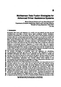
x # 2 = [ x, x&, y, y& ]' = [3500m − 22m / s 6200m 2m / s ] Twelve sensors (4 OOP, 4 LRS, and 4 STT) are randomly distributed around the two targets as illustrated in Fig. 2.

Proc. of SPIE Vol. 7336 73360Y-8 Downloaded From: http://spiedigitallibrary.org/ on 10/22/2013 Terms of Use: http://spiedl.org/terms

(26)

(27)

+

y(m)

+

+

+

- sensor

+ Target #2

++

+

+

Target #1

+

0(00) Fig. 2 Illustration of two moving targets and distributed sensors

We assume there is only one target (agent) in the region of interest (ROI) at the initial stage and all existing sensors are associated with the target. When a new target (the second target) is found in ROI, a new agent will be generated correspondently to represent the new target. At the time, no sensor is allocated to the new agent. Thus, the tracking performance of the new agent is the worst (i.e. covariance accuracy). To improve its tracking performance, the agent with the lowest tracking accuracy has to launch a proposal to the other agent for resources. The agent which has more resources (more sensor information gain), will receive the proposal from the new agent and passively involve in the negotiation. Some resources will be reallocated to the caller and the tracking performance of the receiver might be reduced due to the relocation. To protect the interests of both sides, a game-theoretic scheme is used to guarantee the fairness of the negotiation. When the caller receives some resources (sensors) from the receiver, the tracking accuracy of the caller will be improved due the increase of sensor information gain. The sensor negotiation will be repeated, until the norm of the current covariance matrix of the caller is close to the desired covariance level.

E (k ) = Pd−1 where S is the sensor set of the caller at Time k. Pd

2

2

−

∑H

T −1 i Ri H i

i∈S

(28) 2

is the desired error covariance level and Pd−1 = 2

1 Pd

. When 2

Eq. (28) is close to zero, negotiation is terminated. Sensor # 1 2 3 4 5 6 7 8 9 10 11 12

Table 1: Sensor table Sensor Type x OOP 1000 OOP 800 OOP 1200 OOP 750 LRS 3800 LRS 3300 LRS 2000 LRS 4000 STT 1500 STT 3600 STT 1000 STT 1400

y 1000 2000 2500 6300 6800 3750 3800 3300 5000 3100 6200 7000

where x and y are the position to the global coordinate system. Test #1: In the simulation, we let target’s desired covariance level as 1/10 for Target 1 and 1/25 for Target 2 in the initial stage. 40 TimeSteps are recorded to show the negotiation process between Agent 1 and Agent 2 during target tracking.

Proc. of SPIE Vol. 7336 73360Y-9 Downloaded From: http://spiedigitallibrary.org/ on 10/22/2013 Terms of Use: http://spiedl.org/terms

As we can see from the top-part of Fig. 3, after Agent 2 received some sensors from Agent 1, the E(k) of Target 2 will decrease gradually to zero. At the initial stage, all sensors are associated with Agent 1 and no sensor is assigned to Agent 2. Therefore, in the first several TimeSteps, the three proposals for negotiation are all generated by Agent 2 as shown in the mid-part of Fig. 3. The mid-part of Fig. 3 records the order of the agent to initialize negotiation. 0 means no agents launch a negotiation at time t; 1 means Agent 1 seeks more resources from Agent 2; 2 means Agent 2 asks for more resources from Agent 1.

Sensor Numbenfor Targets

Sresin s Agent

E(k)nsTangen

The changes of sensor number for each agent (target) over time are displayed in the bottom-part of Fig. 3. From the bottom-part of Fig. 3, we can see that for the first negotiation Agent 2 receives two sensors from Agent 1. After the second-round negotiation, another sensor of Agent 1 is assigned to Agent 2. After the third-round negotiation, another four sensors of Agent 1 are assigned to Agent 2. Once E(k) of Agent 2 is close to zero, the negotiation process is terminated. No more negotiation happens for the end of the simulation. Here, we assume a negotiation process will be completed within one TimeStep.

Fig. 3 Two agents and twelve different sensors

Test #2: The first test only considers the sensor reassignment when a new target appears in ROI. Since targets are moving, the distances between the target and sensors will vary over time. In real-life, the signal-to-noise ratio (SNR) of a sensor will increase when the distance of the sensor to a target becomes longer, which means the tracking performance will decrease when a target travels away from the sensors associated to the target. To prevent tracking performance degradation, we need to monitor tracking performance continuously and update the desired covariance level to initialize a new negotiation when necessary. To simulate this scenario, we set different desired covariance levels for the two targets at five different time instances as shown in Table 3. When the desired covariance level is updated during target tracking, a new round of negotiations will start to reallocate resources for enhanced tracking performance. When the objective of both agents is satisfied, the negotiation will stop. Time 1 19 39 59 79

Table 3: Desired Covariance Levels Target 1 Target 2 1/15 1/10 1/10 1/20 1/10 1/30 1/20 1/20 1/30 1/10

Fig. 4 shows the process when the desired covariance levels are reset at five different time instances. At Time instance #1 (the initial stage), the covariance levels of Target 1 and Target 2 are set to 1/15 and 1/10 respectively. Agent 2 launches negotiation request to Agent 1 and receives two sensors from Agent 1 to satisfy its desired covariance level. Since the desired covariance levels of both targets are satisfied, no negotiation has happened. At Time instance #19 and Time instance #39, the desired covariance levels of the two targets are updated. Thus, two new rounds of negotiations

Proc. of SPIE Vol. 7336 73360Y-10 Downloaded From: http://spiedigitallibrary.org/ on 10/22/2013 Terms of Use: http://spiedl.org/terms

are initiated. As the result of negotiations, sensor number of Agent 1 changes to 7 and 8 and sensor number of Agent 2 changes to 5 and 4 after Time instance #19 and Time instance #39. At Time instance #59, the covariance level of Target 1 is changed to 1/20 and the covariance level of Target 2 becomes 1/20, Agent 2 launch one negotiation proposal to Agent 1 and Agent 1 launches two negotiation requests to Agent 2 after Agent 2’s proposal. The final results are 5 sensors for Agent 1 and 7 sensors for Agent 2. After Time instance #79, the two agents begin another round sensor reassignment when their desired covariance level is updated again. From the testing results displayed in Fig. 4 and listed in Table 4, 5, 6, 7, and 8, we can see that our proposed game-theoretical scheme works well for different situations.

U

30

I--- Thrget#1 solid

20

10

0

10

20

30

40

00

60

70

80

90

100

Time etepe

Fig. 4 Satisfying the desired covariance levels for all targets via different-type sensors (OOP, LRS, and STT sensors) Table 4 Sensor assignment after Time instance #0 OOP LRS Target 1 3 3 Target 2 1 1

STT 4 0

Table 5 Sensor assignment after Time instance #19 OOP LRS Target 1 2 2 Target 2 2 2

STT 3 1

Table 6 Sensor assignment after Time instance #39 OOP LRS Target 1 1 1 Target 2 3 3

STT 2 2

Table 7 Sensor assignment after Time instance #59 OOP LRS Target 1 2 2 Target 2 2 2

STT 1 3

Table 8 Sensor assignment after Time instance #79 OOP LRS Target 1 3 3 Target 2 1 1

STT 2 2

Proc. of SPIE Vol. 7336 73360Y-11 Downloaded From: http://spiedigitallibrary.org/ on 10/22/2013 Terms of Use: http://spiedl.org/terms

4. CONCLUSIONS A agent-based game-theoretic negotiation approach for decentralized sensor management (ANGADS) is presented for multiple sensor, multi-modal, multi-target tracking. In the ANGADS approach, we create an agent for each target and deploy sensor management via the negotiations between agents. By incorporating subgame Nash Equilibrium into negotiation, the benefits of all agents in the system will be considered and system performance enhanced over track accuracy (i.e. covariance), timeliness, target identification confidence, and throughput information utility. We have formulated two scenarios and performed simulation tests with three different sensor models. The test results illustrate the applicability of the proposed ANGADS approach.

ACKNOLEDGEMENTS This research was supported in part by the US Air Force under contract number FA8650-08-C-1407. The views and conclusions contained herein are those of the authors and should not be interpreted as necessarily representing the official policies or endorsements, either expressed or implied, of the Air Force.

REFERENCES [1] M. K. Kalandros, L. Trailovic, L. Y. Pao, and Y. Bar Shalom, “Tutorial on multisensory management and fusion algorithms for target tracking,” Proceeding of the 2004 American Control Conference, Boston, MA, pp. 4734-4748, 2004. [2] M. Kalandros and L. Y. Pao, “Covariance control for multisensor systems,” IEEE Transactions on Aerospace and Electronic Systems, Vol. 38, No. 4, Oct. 2002. [3] W. Schmaedeke, “Information-based sensor management,” Proceeding of SPIE, Vol. 1955, 1993. [4] M. Wei, G. Chen, E. Blasch, H. Chen, and J.B. Cruz, Game Theoretic Multiple Mobile Sensor Management under Adversarial Environments,” Fusion 2008, Cologne, Germany, 2008. [5] J. Nash, “Optimal allocation of tracking resources,” Proceeding of IEEE conference on Decision and Control, New Orleans, pp. 1177-1180, 1977. [6] Y. Bar-Shalom and X. Li, Multitarget-Multisensor Tracking: Principles and Techniques, YBS Publishing, 1995. [7] T. Kirubarajan, Y. Bar-shalom, W. D. Blair, and G. A. Watson, “LMMPDAF for Radar Management and Tracking Benchmark with ECM,” IEEE Transactions on Aerospace and Electronic Systems, Vol. 34, No. 4, pp. 2616-2620, 1995. [8] G. A. Watson, W. D. Blair, and T. R. Rice, “Enhanced Electronically Scanned Array Resources Management through Multisensor Integration,” Proceedings of SPIE Conference Signal Processing of Small Target, Vol. 3163, Orlando, FL, pp. 329340, 1997. [9] J. Manyika, An Information Theoretic Approach to Data Fusion and Sensor Management, PhD thesis, The University of Oxford, 1993. [10] J. Manyikia and H. F. Durrant-Whyte, Data Fusion and Sensor Management: An Information-Theoretic Approach, Prentice Hall, 1994. [11] B. S. Y. Rao, H. Durrant-Whyte, and A. Sheen, “A Fully Decentralized Multisensor System for Tracking and Surveillance,” International Journal of Robotics Research, 12(1):20-45, 1991. [12] S. Utete, A Network Manager for a Decentralized Sensing System, Master’s thesis, University of Oxford, 1992. [13] H. Durrant-Whyte and M. Stevens, “Data fusion in decentralized sensing networks,” International Conference on Information Fusion, 2001. [14] N. Xiong, H. Christensen, and P. Svensson, “Reactive tuning of target estimate accuracy in multi-sensor data fusion,” An International Journal on Cybernetics and Systems, Vol. 38, pp. 83-103, 2007. [15] J. Nash, “Two-person cooperative games,” Econometrica, Vol. 21, pp. 128-140, 1953. [16] M. Osborne and A. Rubinstein, A course in game theory, Cambridge, Massachusetts: MIT Press, 1994. [17] I. Kadar, K.C. Chang, K. O’Connor and M. Liggins, “Figures-of-Merit to bridge fusion, long term prediction and dynamic sensor management”, Signal Processing, Sensor Fusion and Target Recognition XIII, Ed. Ivan Kadar, Proc. SPIE Vol. 5429, 2004 [18] Z. Han etal, “Fair Multiuser Channel Allocation for OFDMA Networks Using Nash Bargaining Solutions and Coalitions”, IEEE Trans. On Communications, Vol. 53, 2005 [19] C. Touati, etal, “Generalized Nash Bargaining Solution for Bandwidth Allocation”, Computer Networks, Vol. 50, 2006 [20] K.J. Hintz and E.S. McVey, “Multi-Process Constrained Estimation,” IEEE Trans. on SMC, Vol. 21, No. 1, pp. 237-244, January/February 1991. [21] G.A. McIntyre and K.J. Hintz, “An Information Theoretic Approach to Sensor Scheduling,” Proceedings Signal Processing, Sensor Fusion and Target Recognition VI, Ivan Kadar Editor, Proc. SPIE Vol. 3068, pp. 21-24, April 1997.

Proc. of SPIE Vol. 7336 73360Y-12 Downloaded From: http://spiedigitallibrary.org/ on 10/22/2013 Terms of Use: http://spiedl.org/terms