Aug 22, 2016 - Many approaches for estimation of Remaining Useful Life. (RUL) of a machine, using its operational sensor data, make assumptions about how ...
Multi-Sensor Prognostics using an Unsupervised Health Index based on LSTM Encoder-Decoder Pankaj Malhotra, Vishnu TV, Anusha Ramakrishnan Gaurangi Anand, Lovekesh Vig, Puneet Agarwal, Gautam Shroff TCS Research, New Delhi, India
arXiv:1608.06154v1 [cs.LG] 22 Aug 2016
{malhotra.pankaj, vishnu.tv, anusha.ramakrishnan}@tcs.com {gaurangi.anand, lovekesh.vig, puneet.a, gautam.shroff}@tcs.com
ABSTRACT Many approaches for estimation of Remaining Useful Life (RUL) of a machine, using its operational sensor data, make assumptions about how a system degrades or a fault evolves, e.g., exponential degradation. However, in many domains degradation may not follow a pattern. We propose a Long Short Term Memory based Encoder-Decoder (LSTM-ED) scheme to obtain an unsupervised health index (HI) for a system using multi-sensor time-series data. LSTM-ED is trained to reconstruct the time-series corresponding to healthy state of a system. The reconstruction error is used to compute HI which is then used for RUL estimation. We evaluate our approach on publicly available Turbofan Engine and Milling Machine datasets. We also present results on a real-world industry dataset from a pulverizer mill where we find significant correlation between LSTM-ED based HI and maintenance costs.
1.
INTRODUCTION
Industrial Internet has given rise to availability of sensor data from numerous machines belonging to various domains such as agriculture, energy, manufacturing etc. These sensor readings can indicate health of the machines. This has led to increased business desire to perform maintenance of these machines based on their condition rather than following the current industry practice of time-based maintenance. It has also been shown that condition-based maintenance can lead to significant financial savings. Such goals can be achieved by building models for prediction of remaining useful life (RUL) of the machines, based on their sensor readings. Traditional approach for RUL prediction is based on an assumption that the health degradation curves (drawn w.r.t. time) follow specific shape such as exponential or linear. Under this assumption we can build a model for health index (HI) prediction, as a function of sensor readings. Extrapolation of HI is used for prediction of RUL [29, 24, 25]. However, we observed that such assumptions do not hold in the real-world datasets, making the problem harder to solve. Some of the important challenges in solving the prognostics problem are: i) health degradation curve may not necessarily follow a fixed shape, ii) time to reach same level of degradation by machines of same specifications is often different, iii) each instance has a slightly different initial health or wear, iv) sensor readings if available are Presented at 1st ACM SIGKDD Workshop on Machine Learning for Prognostics and Health Management, San Francisco, CA, USA, 2016. Copyright 2016 Tata Consultancy Services Ltd.
noisy, v) sensor data till end-of-life is not easily available because in practice periodic maintenance is performed. Apart from the health index (HI) based approach as described above, mathematical models of the underlying physical system, fault propagation models and conventional reliability models have also been used for RUL estimation [5, 26]. Data-driven models which use readings of sensors carrying degradation or wear information such as vibration in a bearing have been effectively used to build RUL estimation models [28, 29, 37]. Typically, sensor readings over the entire operational life of multiple instances of a system from start till failure are used to obtain common degradation behavior trends or to build models of how a system degrades by estimating health in terms of HI. Any new instance is then compared with these trends and the most similar trends are used to estimate the RUL [40]. LSTM networks are recurrent neural network models that have been successfully used for many sequence learning and temporal modeling tasks [12, 2] such as handwriting recognition, speech recognition, sentiment analysis, and customer behavior prediction. A variant of LSTM networks, LSTM encoder-decoder (LSTM-ED) model has been successfully used for sequence-to-sequence learning tasks [8, 34, 4] like machine translation, natural language generation and reconstruction, parsing, and image captioning. LSTM-ED works as follows: An LSTM-based encoder is used to map a multivariate input sequence to a fixed-dimensional vector representation. The decoder is another LSTM network which uses this vector representation to produce the target sequence. We provide further details on LSTM-ED in Sections 4.1 and 4.2. LSTM Encoder-decoder based approaches have been proposed for anomaly detection [21, 23]. These approaches learn a model to reconstruct the normal data (e.g. when machine is in perfect health) such that the learned model could reconstruct the subsequences which belong to normal behavior. The learnt model leads to high reconstruction error for anomalous or novel subsequences, since it has not seen such data during training. Based on similar ideas, we use Long Short-Term Memory [14] Encoder-Decoder (LSTM-ED) for RUL estimation. In this paper, we propose an unsupervised technique to obtain a health index (HI) for a system using multi-sensor time-series data, which does not make any assumption on the shape of the degradation curve. We use LSTM-ED to learn a model of normal behavior of a system, which is trained to reconstruct multivariate time-series corresponding to normal behavior. The reconstruction error at a point in a time-series is used
to compute HI at that point. In this paper, we show that: • LSTM-ED based HI learnt in an unsupervised manner is able to capture the degradation in a system: the HI decreases as the system degrades. • LSTM-ED based HI can be used to learn a model for RUL estimation instead of relying on domain knowledge, or exponential/linear degradation assumption, while achieving comparable performance. The rest of the paper is organized as follows: We formally introduce the problem and provide an overview of our approach in Section 2. In Section 3, we describe Linear Regression (LR) based approach to estimate the health index and discuss commonly used assumptions to obtain these estimates. In Section 4, we describe how LSTM-ED can be used to learn the LR model without relying on domain knowledge or mathematical models for degradation evolution. In Section 5, we explain how we use the HI curves of train instances and a new test instance to estimate the RUL of the new instance. We provide details of experiments and results on three datasets in Section 6. Finally, we conclude with a discussion in Section 8, after a summary of related work in Section 7.
2.
APPROACH OVERVIEW
We consider the scenario where historical instances of a system with multi-sensor data readings till end-of-life are available. The goal is to estimate the RUL of a currently operational instance of the system for which multi-sensor data is available till current time-instance. More formally, we consider a set of train instances U of a system. For each instance u ∈ U , we consider a multivariate (u) (u) (u) time-series of sensor readings X (u) = [x1 x2 ... xL(u) ] (u) with L cycles where the last cycle corresponds to the (u) end-of-life, each point xt ∈ Rm is an m-dimensional vector corresponding to readings for m sensors at time-instance t. The sensor data is z-normalized such that the sensor reading (u) xtj at time t for jth sensor for instance u is transformed to (u)
xtj −µj
, where µj and σj are mean and standard deviation σj for the jth sensor’s readings over all cycles from all instances in U . (Note: When multiple modes of normal operation exist, each point can normalized based on the µj and σj for that mode of operation, as suggested in [39].) A subsequence of length l for time-series X (u) starting from time instance t (u) (u) (u) is denoted by X (u) (t, l) = [xt xt+1 ... xt+l−1 ] with 1 ≤ t ≤ L(u) − l + 1. In many real-world multi-sensor data, sensors are correlated. As in [39, 24, 25], we use Principal Components Analysis to obtain derived sensors from the normalized sensor data with reduced linear correlations between them. The multivariate time-series for the derived sensors is (u) (u) (u) (u) represented as Z (u) = [z1 z2 ... zL(u) ], where zt ∈ Rp , p is the number of principal components considered (The best value of p can be obtained using a validation set). ∗ For a new instance u∗ with sensor readings X (u ) over (u∗ ) L cycles, the goal is to estimate the remaining useful ∗ life R(u ) in terms of number of cycles, given the time-series data for train instances {X (u) : u ∈ U }. We describe our approach assuming same operating regime for the entire life of the system. The approach can be easily extended to
multiple operating regimes scenario by treating data for each regime separately (similar to [39, 17]), as described in one of our case studies on milling machine dataset in Section 6.3.
3.
LINEAR REGRESSION BASED HEALTH INDEX ESTIMATION (u)
(u)
(u)
Let H (u) = [h1 h2 ... hL(u) ] represent the HI curve H (u) (u)
for instance u, where each point ht ∈ R, L(u) is the total (u) number of cycles. We assume 0 ≤ ht ≤ 1, s.t. when u is (u) in perfect health ht = 1, and when u performs below an (u) acceptable level (e.g. instance is about to fail), ht = 0. (u) (u) Our goal is to construct a mapping fθ : zt → ht s.t. (u)
(u)
fθ (zt ) = θ T zt
+ θ0
(1) (u)
where θ ∈ Rp , θ0 ∈ R, which computes HI ht from (u) the derived sensor readings zt at time t for instance u. Given the target HI curves for the training instances, the parameters θ and θ0 are estimated using Ordinary Least Squares method.
3.1
Domain-specific target HI curves
The parameters θ and θ0 of the above mentioned Linear Regression (LR) model (Eq. 1) are usually estimated by assuming a mathematical form for the target H (u) , with an exponential function being the most common and successfully employed target HI curve (e.g. [10, 33, 40, 29, 6]), which assumes the HI at time t for instance u as � � log(β).(L(u) − t) (u) , t ∈ [β.L(u) , (1−β).L(u) ]. ht = 1−exp (1 − β).L(u) (2) 0 < β < 1. The starting and ending β fraction of cycles are assigned values of 1 and 0, respectively. Another possible assumption is: assume target HI values of 1 and 0 for data corresponding to healthy condition and failure conditions, respectively. Unlike the exponential HI curve which uses the entire time-series of sensor readings, the sensor readings corresponding to only these points are used to learn the regression model (e.g. [38]). The estimates θˆ and θˆ0 based on target HI curves for train instances are used to obtain the final HI curves H (u) for all the train instances and a new test instance for which RUL is to be estimated. The HI curves thus obtained are used to estimate the RUL for the test instance based on similarity of train and test HI curves, as described later in Section 5.
4.
LSTM-ED BASED TARGET HI CURVE
We learn an LSTM-ED model to reconstruct the time-series of the train instances during normal operation. For example, any subsequence corresponding to starting few cycles when the system can be assumed to be in healthy state can be used to learn the model. The reconstruction model is then used to reconstruct all the subsequences for all train instances and the pointwise reconstruction error is used to obtain a target HI curve for each instance. We briefly describe LSTM unit and LSTM-ED based reconstruction model, and then explain how the reconstruction errors obtained from this model are used to obtain the target HI curves.
Figure 1: RUL estimation steps using unsupervised HI based on LSTM-ED.
4.1
LSTM unit
An LSTM unit is a recurrent unit that uses the input zt , the hidden state activation at−1 , and memory cell activation ct−1 to compute the hidden state activation at at time t. It uses a combination of a memory cell c and three types of gates: input gate i, forget gate f , and output gate o to decide if the input needs to be remembered (using input gate), when the previous memory needs to be retained (forget gate), and when the memory content needs to be output (using output gate). Many variants and extensions to the original LSTM unit as introduced in [14] exist. We use the one as described in [42]. Consider Tn1 ,n2 : Rn1 → Rn2 is an affine transform of the form z 7→ Wz + b for matrix W and vector b of appropriate dimensions. The values for input gate i, forget gate f , output gate o, hidden state a, and cell activation c at time t are computed using the current input zt , the previous hidden state at−1 , and memory cell value ct−1 as given by Eqs. 3-5. σ it ft σ Tm+n,4n = ot σ gt tanh
zt at−1
! (3)
Here σ(z) = 1+e1−z and tanh(z) = 2σ(2z) − 1. The operations σ and tanh are applied elementwise. The four equations from the above simplifed matrix notation read as: it = σ(W1 zt + W2 at−1 + bi ), etc. Here, xt ∈ Rm , and all others it , ft , ot , gt , at , ct ∈ Rn .
4.2
ct = ft ct−1 + it gt
(4)
at = ot tanh(ct )
(5)
Reconstruction Model
We consider sliding windows to obtain L − l + 1 subsequences for a train instance with L cycles. LSTM-ED is trained to reconstruct the normal (healthy) subsequences of length l from all the training instances. The LSTM encoder learns a fixed length vector representation of the input time-series and the LSTM decoder uses this representation to reconstruct the time-series using the current hidden state and the value predicted at the previous time-step. Given (E) a time-series Z = [z1 z2 ... zl ], at is the hidden state of (E) encoder at time t for each t ∈ {1, 2, ..., l}, where at ∈ Rc , c is the number of LSTM units in the hidden layer of the
Figure 2: LSTM-ED inference steps for input {z1 , z2 , z3 } to predict {z0 1 , z0 2 , z0 3 } encoder. The encoder and decoder are jointly trained to reconstruct the time-series in reverse order (similar to [34]), i.e., the target time-series is [zl zl−1 ... z1 ]. (Note: We consider derived sensors from PCA s.t. m = p and n = c in Eq. 3.) Fig. 2 depicts the inference steps in an LSTM-ED reconstruction model for a toy sequence with l = 3. The (E) value xt at time instance t and the hidden state at−1 of the encoder at time t − 1 are used to obtain the hidden state (E) (E) at of the encoder at time t. The hidden state al of the encoder at the end of the input sequence is used as the initial (D) (D) (E) state al of the decoder s.t. al = al . A linear layer with weight matrix w of size c × m and bias vector b ∈ Rm (D) on top of the decoder is used to compute z0t = wT at + b. During training, the decoder uses zt as input to obtain (D) the state at−1 , and then predict z0 t−1 corresponding to target zt−1 . During inference, the predicted value z0 t is (D) input to the decoder to obtain at−1 and predict z0 t−1 . The (u) (u) reconstruction error et for a point zt is given by: (u)
et
(u)
= kzt
(u)
− z0 t k
(6)
The model is trained to minimize the objective E = P Pl (u) 2 It is to be noted that for training, u∈U t=1 (et ) . only the subsequences which correspond to perfect health of an instance are considered. For most cases, the first few operational cycles can be assumed to correspond to healthy state for any instance.
4.3
Reconstruction Error based Target HI
A point zt in a time-series Z is part of multiple
Figure 3: Example of RUL estimation using HI curve matching taken from Turbofan Engine dataset (refer Section 6.2) overlapping subsequences, and is therefore predicted by multiple subsequences Z(j, l) corresponding to j = t − l + 1, t − l + 2, ..., t. Hence, each point in the original time-series for a train instance is predicted as many times as the number of subsequences it is part of (l times for each point except for points zt with t < l or t > L − l which are predicted fewer number of times). An average of all the predictions for a point is taken to be final prediction for that point. The difference in actual and predicted values for a point is used as an unnormalized HI for that point. (u) (u) Error et is normalized to obtain the target HI ht as: (u)
ht (u)
=
(u)
(u)
(u)
(u)
eM − et
eM − em
(7)
(u)
where eM and em are the maximum and minimum values of reconstruction error for instance u over t = 1 2 ... L(u) , respectively. The target HI values thus obtained for all train instances are used to obtain the estimates θˆ and θˆ0 (see Eq. (u) (u) 1). Apart from et , we also consider (et )2 to obtain target HI values for our experiments in Section 6 such that large reconstruction errors imply much smaller HI value.
5.
RUL ESTIMATION USING HI CURVE MATCHING
Similar to [39, 40], the HI curve for a test instance u∗ is compared to the HI curves of all the train instances u ∈ U . The test instance and train instance may take different number of cycles to reach the same degradation level (HI value). Fig. 3 shows a sample scenario where HI curve for a test instance is matched with HI curve for a train instance by varying the time-lag. The time-lag which corresponds to minimum Euclidean distance between the HI curves of the train and test instance is shown. For a given time-lag, the number of remaining cycles for the train instance after the last cycle of the test instance gives the RUL estimate for the test instance. Let u∗ be a test instance and u be a train instance. Similar to [29, 9, 13], we take into account the following scenarios for curve matching based RUL estimation: 1) Varying initial health across instances: The initial health of an instance varies depending on various factors such as the inherent inconsistencies in the manufacturing process. We assume initial health to be close to 1. In order to ensure this, the HI values for an instance are divided by the average of its first few HI values (e.g. first 5% cycles). Also, while ∗ comparing HI curves H (u ) and H (u) , we allow for a time-lag
t such that the∗ HI values of u∗ may be close to the HI values of H (u) (t, L(u ) ) at time t such that t ≤ τ (see Eqs. 8-10). This takes care of instance specific variances in degree of initial wear and degradation evolution. 2) Multiple time-lags with high similarity: The HI curve ∗ H (u ) may have high similarity with H (u) (t, L(u∗) ) for multiple values of time-lag t. We consider multiple RUL estimates for u∗ based on total life of u, rather than considering only the RUL estimate corresponding to the time-lag t with minimum Euclidean distance between ∗ ∗ the curves H (u ) and H (u) (t, L(u ) ). The multiple RUL estimates corresponding to each time-lag are assigned weights proportional to the similarity of the curves to get the final RUL estimate (see Eq. 10). 3) Non-monotonic HI : Due to inherent noise in sensor readings, HI curves obtained using LR are non-monotonic. To reduce the noise in the estimates of HI, we use moving average smoothening. 4) Maximum value of RUL estimate: When an instance is in very good health or has been operational for few cycles, estimating RUL is difficult. We limit the maximum RUL estimate for any test instance to Rmax . Also, the maximum RUL estimate for the instance u∗ based on HI ∗ curve comparison with instance u is limited by L(u) − L(u ) . This implies that the maximum RUL estimate ∗for any ∗test ˆ (u ) + L(u ) ≤ instance u will be such that the total length R Lmax , where Lmax is the maximum length for any training instance available. Fewer the number of cycles available for a test instance, more difficult it becomes to estimate the RUL. We define similarity between HI curves of test instance u∗ and train instance u with time-lag t as: s(u∗ , u, t) = exp(−d2 (u∗ , u, t)/λ)
(8)
where, ∗
2
∗
d (u , u, t) =
1 L(u∗ )
(u ) LX
(u∗ )
(hi
(u)
− hi+t )2
(9)
i=1 ∗
∗
is the squared Euclidean distance between H (u ) (1, L(u ) ) ∗ ∗ and H (u) (t, L(u ) ), and λ > 0, t ∈ {1, 2, ..., τ }, t + L(u ) ≤ L(u) . Here, λ controls the notion of similarity: a small value of λ would imply large difference in s even when d is not large. The RUL estimate for u∗ based on the HI curve for u ˆ (u∗ ) (u, t) = L(u) − L(u∗ ) − t. and for time-lag t is given by R ˆ (u∗ ) (u, t) is assigned a weight of s(u∗ , u, t) The estimate R ˆ (u∗ ) for R(u∗ ) is such that the weighted average estimate R given by P ˆ (u∗ ) (u, t) ∗ s(u∗ , u, t).R ˆ (u ) = P R (10) s(u∗ , u, t) where the summation is over only those combinations of u and t which satisfy s(u∗ , u, t) ≥ α.smax , where smax = maxu∈U,t∈{1 ... τ } {s(u∗ , u, t)}, 0 ≤ α ≤ 1. It is to be noted that the parameter α decides the number ˆ (u∗ ) (u, t) to be considered to get the final of RUL estimates R ˆ (u∗ ) . Also, variance of the RUL estimates RUL estimate R ∗ (u ) ˆ ˆ (u∗ ) can be used as R (u, t) considered for computing R a measure of confidence in the prediction, which is useful in practical applications (for example, see Section 6.2.2). During the initial stages of an instance’s usage, when it is in good health and a fault has still not appeared, estimating
RUL is tough, as it is difficult to know beforehand how exactly the fault would evolve over time once it appears.
Reconstruction Error
6.
5 4
EXPERIMENTAL EVALUATION
We evaluate our approach on two publicly available datasets: C-MAPSS Turbofan Engine Dataset [33] and Milling Machine Dataset [1], and a real world dataset from a pulverizer mill. For the first two datasets, the ground truth in terms of the RUL is known, and we use RUL estimation performance metrics to measure efficacy of our algorithm (see Section 6.1). The Pulverizer mill undergoes repair on timely basis (around one year), and therefore ground truth in terms of actual RUL is not available. We therefore draw comparison between health index and the cost of maintenance of the mills. For the first two datasets, we use different target HI curves for learning the LR model (refer Section 3): LR-Lin and LR-Exp models assume linear and exponential form for the target HI curves, respectively. LR-ED1 and LR-ED2 use normalized reconstruction error and normalized squared-reconstruction error as target HI (refer Section 4.3), respectively. The target HI values for LR-Exp are obtained using Eq. 2 with β = 5% as suggested in [40, 39, 29].
6.1
Performance metrics considered
Several metrics have been proposed for evaluating the performance of prognostics models [32]. We measure the performance in terms of Timeliness Score (S), Accuracy (A), Mean Absolute Error (MAE), Mean Squared Error (MSE), and Mean Absolute Percentage Error (MAPE1 and MAPE2 ) as mentioned in Eqs. 11-15, respectively. For test instance (u∗ ) ˆ (u∗ ) − R(u∗ ) between the estimated u∗ , the error ∆ = R ˆ (u∗ ) ) and actual RUL (R(u∗ ) ). The score S used to RUL (R measure the performance of a model is given by: S=
N X
∗
(exp(γ.|∆(u ) |) − 1)
(11)
u∗ =1 ∗
where γ = 1/τ1 if ∆(u ) < 0, else γ = 1/τ2 . Usually, τ1 > τ2 such that late predictions are penalized more compared to early predictions. The lower the value of S, the better is the performance.
A=
N ∗ 100 X I(∆(u ) ) N u∗ =1
∗
∗
where I(∆(u ) ) = 1 if ∆(u τ1 > 0, τ2 > 0.
M AE =
)
(12) ∗
∈ [−τ1 , τ2 ], else I(∆(u ) ) = 0,
N N ∗ ∗ 1 X 1 X |∆(u ) |, M SE = (∆(u ) )2 N u∗ =1 N u∗ =1
(13)
∗
N 100 X |∆(u ) | N u∗ =1 R(u∗ )
(14)
∗ N |∆(u ) | 100 X N u∗ =1 R(u∗ ) + L(u∗ )
(15)
M AP E1 =
M AP E2 =
∗
A prediction is considered a false positive (FP) if ∆(u ∗ −τ1 , and false negative (FN) if ∆(u ) > τ2 .
)
tE ) 0.25 0.57 0.43
tC 7 7 7
P(C>tC | E>tE ) 0.61 0.84 0.75
E (last day) 2.4 8.0 16.2
C(Mi ) 92 279 209
Table 3: Pulverizer Mill: Correlation between reconstruction error E and maintenance cost C(Mi ). the days of a year between any two consecutive time-based maintenances Mi and Mi+1 , and use the corresponding subsequences for learning LSTM-ED models. This data is divided into training and validation sets. A different LSTM-ED model is learnt after each maintenance. The architecture with minimum average reconstruction error over a validation set is chosen as the best model. The best models learnt using data after M0 , M1 and M2 are obtained for c = 40, 20, and 100, respectively. The LSTM-ED based reconstruction error for each day is z-normalized using the mean and standard deviation of the reconstruction errors over the sequences in validation set. From the results in Table 3, we observe that average reconstruction error E on the last day before M1 is the least, and so is the cost C(M1 ) incurred during M1 . For M2 and M3 , E as well as corresponding C(Mi ) are higher compared to those of M1 . Further, we observe that for the days when average value of reconstruction error E > tE , a large fraction (>0.61) of them have a high ongoing maintenance cost C > tC . The significant correlation between reconstruction error and cost incurred suggests that the LSTM-ED based reconstruction error is able to capture the health of the mill.
7.
RELATED WORK
Similar to our idea of using reconstruction error for modeling normal behavior, variants of Bayesian Networks have been used to model the joint probability distribution over the sensor variables, and then using the evidence probability based on sensor readings as an indicator of normal behaviour (e.g. [11, 35]). [25] presents an unsupervised approach which does not assume a form for the HI curve and uses discrete Bayesian Filter to recursively estimate the health index values, and then use the k-NN classifier to find the most similar offline models. Gaussian Process Regression (GPR) is used to extrapolate the HI curve if the best class-probability is lesser than a threshold. Recent review of statistical methods is available in [31, 36, 15]. We use HI Trajectory Similarity Based Prediction (TSBP) for RUL estimation similar to [40] with the key difference being that the model proposed in [40] relies on exponential assumption to learn a regression model for HI estimation, whereas our approach uses LSTM-ED based HI to learn the regression model. Similarly, [29] proposes RULCLIPPER (RC) which to the best of our knowledge has shown the best performance on C-MAPSS when compared to various approaches evaluated using the dataset [31]. RC tries various combinations of features to select the best set of features and learns linear regression (LR) model over these features to predict health index which is mapped to a HI polygon, and similarity of HI polygons is used instead of univariate curve matching. The parameters of LR model are estimated by assuming exponential target HI (refer Eq. 2). Another variant of TSBP [39] directly uses multiple PCA sensors for multi-dimensional curve matching which is used for RUL estimation, whereas we obtain a univariate HI by taking a weighted combination of the PCA sensors learnt
using the unsupervised HI obtained from LSTM-ED as the target HI. Similarly, [20, 19] learn a composite health index based on the exponential assumption. Many variants of neural networks have been proposed for prognostics (e.g. [3, 27, 13, 18]): very recently, deep Convolutional Neural Networks have been proposed in [3] and shown to outperform regression methods based on Multi-Layer Perceptrons, Support Vector Regression and Relevance Vector Regression to directly estimate the RUL (see Table 4 for performance comparison with our approach on the Turbofan Engine dataset). The approach uses deep CNNs to learn higher level abstract features from raw sensor values which are then used to directly estimate the RUL, where RUL is assumed to be constant for a fixed number of starting cycles and then assumed to decrease linearly. Similarly, Recurrent Neural Network has been used to directly estimate the RUL [13] from the time-series of sensor readings. Whereas these models directly estimate the RUL, our approach first estimates health index and then uses curve matching to estimate RUL. To the best of our knowledge, our LSTM Encoder-Decoder based approach performs significantly better than Echo State Network [27] and deep CNN based approaches [3] (refer Table 4). Reconstruction models based on denoising autoencoders [23] have been proposed for novelty/anomaly detection but have not been evaluated for RUL estimation task. LSTM networks have been used for anomaly/fault detection [22, 7, 41], where deep LSTM networks are used to learn prediction models for the normal time-series. The likelihood of the prediction error is then used as a measure of anomaly. These models predict time-series in the future and then use prediction errors to estimate health or novelty of a point. Such models rely on the the assumption that the normal time-series should be predictable, whereas LSTM-ED learns a representation from the entire sequence which is then used to reconstruct the sequence, and therefore does not depend on the predictability assumption for normal time-series.
8.
DISCUSSION
We have proposed an unsupervised approach to estimate health index (HI) of a system from multi-sensor time-series data. The approach uses time-series instances corresponding to healthy behavior of the system to learn a reconstruction model based on LSTM Encoder-Decoder (LSTM-ED). We then show how the unsupervised HI can be used for estimating remaining useful life instead of relying on domain knowledge based degradation models. The proposed approach shows promising results overall, and in some cases performs better than models which rely on assumptions about health degradation for the Turbofan Engine and Milling Machine datasets. Whereas models relying on assumptions such as exponential health degradation cannot attune themselves to instance specific behavior, the LSTM-ED based HI uses the temporal history of sensor readings to predict the HI at a point. A case study on real-world industry dataset of a pulverizer mill shows signs of correlation between LSTM-ED based reconstruction error and the cost incurred for maintaining the mill, suggesting that LSTM-ED is able to capture the severity of fault.
9.
REFERENCES
[1] A. Agogino and K. Goebel. Milling data set. BEST lab, UC Berkeley, 2007.
[2] G. Anand, A. H. Kazmi, P. Malhotra, L. Vig, P. Agarwal, and G. Shroff. Deep temporal features to predict repeat buyers. In NIPS 2015 Workshop: Machine Learning for eCommerce, 2015. [3] G. S. Babu, P. Zhao, and X.-L. Li. Deep convolutional neural network based regression approach for estimation of remaining useful life. In Database Systems for Advanced Applications. Springer, 2016. [4] S. Bengio, O. Vinyals, N. Jaitly, and N. Shazeer. Scheduled sampling for sequence prediction with recurrent neural networks. In Advances in Neural Information Processing Systems, 2015. [5] F. Cadini, E. Zio, and D. Avram. Model-based monte carlo state estimation for condition-based component replacement. Reliability Engg. & System Safety, 2009. [6] F. Camci, O. F. Eker, S. Ba¸skan, and S. Konur. Comparison of sensors and methodologies for effective prognostics on railway turnout systems. Proceedings of the Institution of Mechanical Engineers, Part F: Journal of Rail and Rapid Transit, 230(1):24–42, 2016. [7] S. Chauhan and L. Vig. Anomaly detection in ecg time signals via deep long short-term memory networks. In Data Science and Advanced Analytics (DSAA), 2015. 36678 2015. IEEE International Conference on, pages 1–7. IEEE, 2015. [8] K. Cho, B. Van Merri¨enboer, C. Gulcehre, D. Bahdanau, F. Bougares, H. Schwenk, and Y. Bengio. Learning phrase representations using rnn encoder-decoder for statistical machine translation. arXiv preprint arXiv:1406.1078, 2014. [9] J. B. Coble. Merging data sources to predict remaining useful life–an automated method to identify prognostic parameters. 2010. [10] C. Croarkin and P. Tobias. Nist/sematech e-handbook of statistical methods. NIST/SEMATECH, 2006. [11] A. Dubrawski, M. Baysek, M. S. Mikus, C. McDaniel, B. Mowry, L. Moyer, J. Ostlund, N. Sondheimer, and T. Stewart. Applying outbreak detection algorithms to prognostics. In AAAI Fall Symposium on Artificial Intelligence for Prognostics, 2007. [12] A. Graves, M. Liwicki, S. Fern´ andez, R. Bertolami, H. Bunke, and J. Schmidhuber. A novel connectionist system for unconstrained handwriting recognition. Pattern Analysis and Machine Intelligence, IEEE Transactions on, 31(5):855–868, 2009. [13] F. O. Heimes. Recurrent neural networks for remaining useful life estimation. In International Conference on Prognostics and Health Management, 2008. [14] S. Hochreiter and J. Schmidhuber. Long short-term memory. Neural computation, 9(8):1735–1780, 1997. [15] M. Jouin, R. Gouriveau, D. Hissel, M.-C. P´era, and N. Zerhouni. Particle filter-based prognostics: Review, discussion and perspectives. Mechanical Systems and Signal Processing, 2015. [16] R. Khelif, S. Malinowski, B. Chebel-Morello, and N. Zerhouni. Rul prediction based on a new similarity-instance based approach. In IEEE International Symposium on Industrial Electronics, 2014. [17] J. Lam, S. Sankararaman, and B. Stewart. Enhanced trajectory based similarity prediction with uncertainty quantification. PHM 2014, 2014.
[18] J. Liu, A. Saxena, K. Goebel, B. Saha, and W. Wang. An adaptive recurrent neural network for remaining useful life prediction of lithium-ion batteries. Technical report, DTIC Document, 2010. [19] K. Liu, A. Chehade, and C. Song. Optimize the signal quality of the composite health index via data fusion for degradation modeling and prognostic analysis. 2015. [20] K. Liu, N. Z. Gebraeel, and J. Shi. A data-level fusion model for developing composite health indices for degradation modeling and prognostic analysis. Automation Science and Engineering, IEEE Transactions on, 10(3):652–664, 2013. [21] P. Malhotra, A. Ramakrishnan, G. Anand, L. Vig, P. Agarwal, and G. Shroff. Lstm-based encoder-decoder for multi-sensor anomaly detection. 33rd International Conference on Machine Learning, Anomaly Detection Workshop. arXiv preprint arXiv:1607.00148, 2016. [22] P. Malhotra, L. Vig, G. Shroff, and P. Agarwal. Long short term memory networks for anomaly detection in time series. In ESANN, 23rd European Symposium on Artificial Neural Networks, Computational Intelligence and Machine Learning, 2015. [23] E. Marchi, F. Vesperini, F. Eyben, S. Squartini, and B. Schuller. A novel approach for automatic acoustic novelty detection using a denoising autoencoder with bidirectional lstm neural networks. In Acoustics, Speech and Signal Processing (ICASSP). IEEE, 2015. [24] A. Mosallam, K. Medjaher, and N. Zerhouni. Data-driven prognostic method based on bayesian approaches for direct remaining useful life prediction. Journal of Intelligent Manufacturing, 2014. [25] A. Mosallam, K. Medjaher, and N. Zerhouni. Component based data-driven prognostics for complex systems: Methodology and applications. In Reliability Systems Engineering (ICRSE), 2015 First International Conference on, pages 1–7. IEEE, 2015. [26] E. My¨ otyri, U. Pulkkinen, and K. Simola. Application of stochastic filtering for lifetime prediction. Reliability Engineering & System Safety, 91(2):200–208, 2006. [27] Y. Peng, H. Wang, J. Wang, D. Liu, and X. Peng. A modified echo state network based remaining useful life estimation approach. In IEEE Conference on Prognostics and Health Management (PHM), 2012. [28] H. Qiu, J. Lee, J. Lin, and G. Yu. Robust performance degradation assessment methods for enhanced rolling element bearing prognostics. Advanced Engineering Informatics, 17(3):127–140, 2003. [29] E. Ramasso. Investigating computational geometry for failure prognostics in presence of imprecise health indicator: Results and comparisons on c-mapss datasets. In 2nd Europen Confernce of the Prognostics and Health Management Society., 2014. [30] E. Ramasso, M. Rombaut, and N. Zerhouni. Joint prediction of continuous and discrete states in time-series based on belief functions. Cybernetics, IEEE Transactions on, 43(1):37–50, 2013. [31] E. Ramasso and A. Saxena. Performance benchmarking and analysis of prognostic methods for cmapss datasets. Int. J. Progn. Health Manag, 2014. [32] A. Saxena, J. Celaya, E. Balaban, K. Goebel, B. Saha,
[33]
[34]
[35]
[36]
[37] [38]
[39]
[40]
[41]
[42]
S. Saha, and M. Schwabacher. Metrics for evaluating performance of prognostic techniques. In Prognostics and health management, 2008. phm 2008. international conference on, pages 1–17. IEEE, 2008. A. Saxena, K. Goebel, D. Simon, and N. Eklund. Damage propagation modeling for aircraft engine run-to-failure simulation. In Prognostics and Health Management, 2008. PHM 2008. International Conference on, pages 1–9. IEEE, 2008. I. Sutskever, O. Vinyals, and Q. V. Le. Sequence to sequence learning with neural networks. In Z. Ghahramani, M. Welling, C. Cortes, N. D. Lawrence, and K. Q. Weinberger, editors, Advances in Neural Information Processing Systems. 2014. D. Tobon-Mejia, K. Medjaher, and N. Zerhouni. Cnc machine tool’s wear diagnostic and prognostic by using dynamic bayesian networks. Mechanical Systems and Signal Processing, 28:167–182, 2012. K. L. Tsui, N. Chen, Q. Zhou, Y. Hai, and W. Wang. Prognostics and health management: A review on data driven approaches. Mathematical Problems in Engineering, 2015, 2015. P. Wang and G. Vachtsevanos. Fault prognostics using dynamic wavelet neural networks. AI EDAM, 2001. P. Wang, B. D. Youn, and C. Hu. A generic probabilistic framework for structural health prognostics and uncertainty management. Mechanical Systems and Signal Processing, 28:622–637, 2012. T. Wang. Trajectory similarity based prediction for remaining useful life estimation. PhD thesis, University of Cincinnati, 2010. T. Wang, J. Yu, D. Siegel, and J. Lee. A similarity-based prognostics approach for remaining useful life estimation of engineered systems. In Prognostics and Health Management, International Conference on. IEEE, 2008. M. Yadav, P. Malhotra, L. Vig, K. Sriram, and G. Shroff. Ode-augmented training improves anomaly detection in sensor data from machines. In NIPS Time Series Workshop. arXiv preprint arXiv:1605.01534, 2015. W. Zaremba, I. Sutskever, and O. Vinyals. Recurrent neural network regularization. arXiv preprint arXiv:1409.2329, 2014.
APPENDIX A. BENCHMARKS ON ENGINE DATASET Approach LR-ED2 (proposed) RULCLIPPER [29] Bayesian-1 [24] Bayesian-2 [25] HI-SNR [19] ESN-KF [27] EV-KNN [30] IBL [16] Shapelet [16] DeepCNN [3]
S 256 216 NR NR NR NR NR NR 652 1287
A 67 67 NR NR NR NR 53 54 NR NR
MAE 9.9 10.0 NR NR NR NR NR NR NR NR
MSE 164 176 NR NR NR 4026 NR NR NR 340
MAPE1 18 20 12 11 NR NR NR NR NR NR
TURBOFAN MAPE2 5.0 NR NR NR 8 NR NR NR NR NR
FPR 13 56 NR NR NR NR 36 18 NR NR
FNR 20 44 NR NR NR NR 11 28 NR NR
Table 4: Performance of various approaches on Turbofan Engine Data. NR: Not Reported.