Multi-Source and Multi-Directional Shear Wave ... - IEEE Xplore

IEEE Transactions on Ultrasonics, Ferroelectrics, and Frequency Control ,

vol. 62, no. 4,

April

2015

647

Multi-Source and Multi-Directional Shear Wave Generation With Intersecting Steered Ultrasound Push Beams Alireza Nabavizadeh, Student Member, IEEE, Pengfei Song, Member, IEEE, Shigao Chen, Member, IEEE, James F. Greenleaf, Life Member, IEEE, and Matthew W. Urban, Senior Member, IEEE Abstract—Elasticity imaging is becoming established as a means of assisting in diagnosis of certain diseases. Shear wave-based methods have been developed to perform elasticity measurements in soft tissue. Comb-push ultrasound shear elastography (CUSE) is one of these methods that apply acoustic radiation force to induce the shear wave in soft tissues. CUSE uses multiple ultrasound beams that are transmitted simultaneously to induce multiple shear wave sources into the tissue, with improved shear wave SNR and increased shear wave imaging frame rate. We propose a novel method that uses steered push beams (SPB) that can be applied for beam formation for shear wave generation. In CUSE beamforming, either unfocused or focused beams are used to create the propagating shear waves. In SPB methods we use unfocused beams that are steered at specific angles. The interaction of these steered beams causes shear waves to be generated in more of a random nature than in CUSE. The beams are typically steered over a range of 3 to 7° and can either be steered to the left (−θ) or right (+θ).We performed simulations of 100 configurations using Field II and found the best configurations based on spatial distribution of peaks in the resulting intensity field. The best candidates were ones with a higher number of the intensity peaks distributed over all depths in the simulated beamformed results. Then these optimal configurations were applied on a homogeneous phantom and two different phantoms with inclusions. In one of the inhomogeneous phantoms we studied two spherical inclusions with 10 and 20 mm diameters, and in the other phantom we studied cylindrical inclusions with diameters ranging from 2.53 to 16.67 mm. We compared these results with those obtained using conventional CUSE with unfocused and focused beams. The mean and standard deviation of the resulting shear wave speeds were used to evaluate the accuracy of the reconstructions by examining bias with nominal values for the phantoms as well as the contrast-to-noise ratio in the inclusion phantom results. In general the contrast-to-noise ratio (CNR) was higher and the bias was lower using the SPB method compared with the CUSE realizations except in the largest inclusions. In the cylindrical inclusion with 10.4 mm diameter, Manuscript received October 27, 2014; accepted January 21, 2015. This work was supported by grant R01DK092255, R01DK082408, and R01EB002167 from the National Institute of Diabetes and Digestive and Kidney Diseases (NIDDK), National Institute of Biomedical Imaging and Bioengineering (NIBIB), and National Institutes of Health (NIH). The content is solely the responsibility of the authors and does not necessarily represent the official views of the NIDDK, NIBIB, and NIH. Mayo Clinic and the authors have a financial interest in the technology described here. A. Nabavizadeh is with Biomedical Informatics and Computational Biology, University of Minnesota—Rochester, Rochester, Minnesota 55905, USA (e-mail: [email protected]). A. Nabavizadeh, P. Song, S. Chen, J. F. Greenleaf, and M. W. Urban are with the Department of Physiology and Biomedical Engineering, Mayo Clinic College of Medicine, Rochester, Minnesota 55905, USA. DOI http://dx.doi.org/10.1109/TUFFC.2014.006805

the CNR in CUSE methods ranged between 18.52 and 22.02 and the bias ranged between 5.50 and 11.12%, whereas for SPB methods provided CNR values between 23.07 and 48.90 and bias values between 3.78 and 9.22%. In a smaller cylindrical inclusion with diameter of 4.05 mm, CUSE methods gave CNR between 14.69 and 22.28 and bias ranging between 28.95 and 29.28%, whereas the SPB methods provided CNR values between 16.7 and 25.2 and bias values varying from 25.54 to 30.44%. The SPB method provides a flexible framework to produce shear wave sources that are widely distributed within the field-of-view for robust shear wave speed imaging.

I. Introduction

T

he mechanical properties of soft tissue can be characterized using shear wave-based elastography, which is a noninvasive method helping to evaluate the state of tissue health [1]. Ultrasound radiation force can be used to induce motion into tissue, and the resulting shear wave is tracked to characterize the mechanical properties of the tissue [2], [3]. If we assume that the soft tissues are incompressible, isotropic, linear, and elastic, the shear wave propagation speed cs in tissue can be defined as [3]



µ = ρc s2, (1)

where ρ is the mass density and can be assumed for all tissue to be 1000 kg/m3 [4], thus by measuring the shear wave propagation speed it is possible to estimate the shear modulus of tissue. According to these concepts, different methods have been developed. Sarvazyan et al. [1] introduced the shear wave elasticity imaging method based on applying radiation force to generate shear waves and measure their propagation. Since this seminal paper, many methods have been developed to distribute the ultrasound intensity in particular ways to change the acoustic radiation force excitation. Acoustic radiation force impulse methods apply impulsive acoustic radiation force to create shear wave as presented by Nightingale et al. [5]. Bercoff et al. [6], proposed supersonic shear imaging (SSI), which produces a shear wave with sharp wave front and large depth extent from the combination of several separate radiation force pushes positioned at different depths. Chen et al. [7], developed a method called shearwave dispersion ultrasound vibrometry, based on measuring the shear wave propagation speed

0885–3010 © 2015 IEEE. Personal use is permitted, but republication/redistribution requires IEEE permission. See http://www.ieee.org/publications_standards/publications/rights/index.html for more information.

648

IEEE Transactions on Ultrasonics, Ferroelectrics, and Frequency Control ,

in tissue at multiple frequencies to measure both the elasticity and viscosity quantitatively. A method called spatially modulated ultrasound radiation force used unique methods of apodizing and applying focusing delays to array elements to create a shear wave with a known spatial pattern. This approach was used to characterize the shear modulus of the tissue [8]. Another method of generating shear waves was performed by applying the crawling wave technique that results from the interference of oscillation of two traveling waves in opposite directions [9]–[11]. This method used both conventionally focused beams as well as axicon beams. Recently, Zhao et al. [12], reported using an unfocused beam to perform shear wave speed measurements. While the unfocused beam can provide accurate measurements over a large depth-of-field, the resulting waves have smaller displacement compared with those from a focused beam. To account for this shortcoming, Song et al. [13], developed a method called comb push ultrasound shear wave elastography (CUSE), which has the ability to reconstruct a full field-of-view 2-D shear wave speed map in only one rapid data acquisition. To generate shear waves in this method, multiple focused or unfocused beams are arranged in a comb pattern (comb-push). Hybrid beamforming methods presented by Nabavizadeh et al. [14] combine traditional focusing methods and axicon focusing to induce shear wave in tissue with elongated field of view compared with traditional focused beam forming methods. Recently, Lee et al. [15] described a new beamforming method to enhance the shear wave motion by using an axicon beam and aperture apodization to create the push beam used to produce the shear wave, which resulted in a higher SNR and thus higher accuracy in shear wave speed estimation. With any of the aforementioned methods to perform the excitation with acoustic radiation force, the shear wave motion can be analyzed to create an elasticity image. Depending on the excitation, it may be necessary for one or more excitations at different locations to measure the motion throughout the field-of-view (FOV) to estimate the shear wave speed at all spatial locations. One main reason for this is that shear wave attenuation in soft tissues can be significant enough to make it difficult to robustly estimate shear wave speed because the motion may be too small to be reliable. It is therefore a desirable goal to develop a method where shear wave sources can be distributed throughout a FOV so that the effects of shear wave attenuation are diminished. This was one advantage of the CUSE method in terms of distributing shear wave sources within the FOV. However, an even denser distribution of shear wave sources may be able to make better localized shear wave speed measurements. In this paper we introduce new beamforming methods called steered push beam (SPB) methods. The objective of this method is to create multiple foci generated by the

vol. 62, no. 4,

April

2015

interference of different ultrasound push beams to create shear waves. The method uses segments of an ultrasound aperture and applies steering angles to the segments to create overlapping beams that interfere to create multiple focal points that have sufficient intensity to generate shear waves. This method can use focused or unfocused push beams and the steering angles can be assigned in a deterministic or random fashion. This is an alternative method to using single or multiple unfocused or focused push beams to generate a shear wave motion field. The paper will be organized as follows. We will present the methods for designing the ultrasound intensity distributions using deterministic and randomized techniques. We will present results in phantoms that are homogeneous and have spherical and cylindrical inclusions. The paper will be concluded with a discussion and summary. II. Methods For this SPB method we can consider an ultrasound array transducer, either one-dimensional array or twodimensional array. For simplicity, we will describe the one-dimensional array case in detail. The aperture of the array transducer consists of N elements. We can divide this aperture into segments of Ns elements. Each segment can have a transmit profile which assigns an apodization weighting to the amplitude of signals applied to the elements in the segment, a steering angle with either positive or negative signed inclination, as well as a delay profile. We will primarily concentrate the descriptions to the use of unfocused beams, but focused beams could be used as well. These parameters can be determined in a manner to create specific types of beams or configurations, or the parameters can be left for random assignment. We will discuss both the deterministic and random configurations. A. Deterministic Configurations It may be desirable to mimic certain configurations. For example, the CUSE method employs push beams that are deterministically placed in the field-of-view (FOV) to create shear waves from known positions [3], [16]–[17]. With steering we can also generate beams in specified positions as shown in Fig. 1. Such an arrangement can be compared between an unfocused CUSE (U-CUSE) configuration and so-called axicon CUSE (AxCUSE) configuration because one of the beams is formed with an axicon-like arrangement using the steering of +θ and −θ for adjacent segments of elements [14], [18]. The acoustic radiation force density, F, in an absorbing medium can be written as   2αI , (2) F = c

nabavizadeh et al.: multi-source and multi-directional shear wave

649

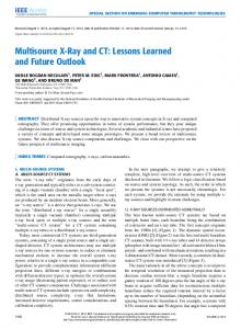
Fig. 1. Schematic drawings for U-CUSE and axicon CUSE.

 where α is the ultrasound attenuation of the medium, I is the ultrasound intensity, and c is the ultrasound speed in the medium. It should be noted that the force and intensity are both vector quantities. The force is proportional to the intensity, so the acoustic radiation force distribution can be explored by simulating the ultrasound intensity using a simulation package such as Field II [19], [20] or FOCUS [21]–[23]. A simulation of the U-CUSE and AxCUSE configurations depicted in Fig. 1 are shown in Fig. 2 for unfocused beams of 16 elements and using θ = 3°. A linear array transducer mimicking the L7–4 transducer (Philips Healthcare, Andover, MA, USA) was used for the simulations using Field II with an ultrasound frequency of 4.0 MHz. Many parameters such as the number of elements, angle of inclination, positions of beam segments, ultrasound frequency, medium ultrasound attenuation, and transducer geometry can be varied to optimize the ultrasound intensity distribution for specific applications. Simulations

of the intensity distributions can be used to explore this wide parameter space for optimal configurations. B. Randomized Configurations It may be advantageous to generate multiple shear wave sources in the FOV for the purposes of creating a multitude of shear waves that are propagating in the medium. Shear wave attenuation in some materials or tissues can be quite significant so shear wave sources may be spaced too far apart to generate shear waves in certain areas in the FOV. Increasing the number of shear wave sources in the FOV provides a higher probability that all areas of the FOV will encounter a propagating shear wave that can be used for later analysis to estimate shear wave velocity or other parameters related to material characterization of elasticity or viscoelasticity. One other consideration is that the acoustic output for push beams can be very high. These levels are regulated

Fig. 2. Intensity simulations. (a) U-CUSE, (b) axicon CUSE. Each of the fields is normalized independently and plotted on a log scale.

650

IEEE Transactions on Ultrasonics, Ferroelectrics, and Frequency Control ,

vol. 62, no. 4,

April

2015

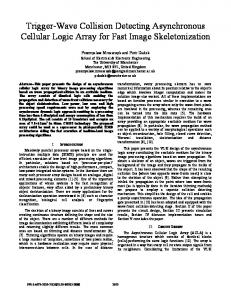
Fig. 3. Results for a random configuration for the angle sign using a fixed θ = 4°. (a) Transmit delays, (b) intensity field.

by the Food and Drug Administration (FDA). To reduce the peak levels of pressure a wider distribution of the ultrasound pressure in the FOV may help to avoid having to reduce input voltage levels and achieve maximum power deposition for shear wave imaging. As an example let the total number of elements N = 128 and the number of elements in a segment be Ns = 8. For each segment an angle of inclination can be assigned as either +θ or −θ. In this example let θ = 4°. The sign of the angle can be randomly assigned such that the signs for each of the segments may be [− − + − − + + − − − + − − + − +]. The sign of the segments can be determined using a random number generator with a starting seed value applied to the number generator so that previously used seeds can be used to obtain the same result with subsequent simulations. The time delays applied to the aperture and the resulting ultrasound intensity field are shown in Fig. 3. In the previous example, the value of θ was fixed and only the sign was allowed to randomly change. Additional-

ly, the value of θ could be allowed to vary over a specified range of values to change the distribution of the intensity in the FOV. In this example, the values of θ were allowed to vary over [3°, 4°, 5°, 6°]. An example of the time delays and resulting ultrasound intensity field is shown in Fig. 4 with the following values for the segments [−4°, −6°, +6°, −6°, −5°, +3°, +6°, −6°, −5°, −5°, +5°, −5°, −5°, +5°, −5°, +3°]. To evaluate for optimal intensity fields we designed an automated method to determine how many foci were created at a given depth in the FOV. The optimal fields will have many foci at each depth such that there are many shear wave sources distributed through depth. For a given intensity field, a region in depth was averaged together over 1 mm, though this segment could be larger. To evaluate the number of foci, represented by peaks in the intensity, we used an averaged profile, In(x,z) using the equation

I m(x, z ) = I n2(x, z ) − I n2(x, z ), (3)

Fig. 4. Results for a random configuration for the angle sign and random angles in the range θ = [3°, 4°, 5°, 6°]. (a) Transmit delays, (b) intensity field.

nabavizadeh et al.: multi-source and multi-directional shear wave

651

Fig. 5. Intensity profiles and spatial Fourier transforms. (a) Spatial profile of Im(x, z) at z = 15 mm, (b) spatial profile of Im(x, z) at z = 25 mm, (c) spatial profile of Im(x, z) at z = 35 mm, (d) spatial Fourier transform of Im(x, z) at z = 15 mm, (e) spatial Fourier transform of Im(x, z) at z = 25 mm, (f) spatial Fourier transform of Im(x, z) at z = 35 mm.



I n2(x, z ) =

1 Nx

Nx

∑

I n2(x, z ), (4)

x =1

where I n2(x, z ) is the mean of the squared average profile. We used the square intensity instead of the intensity to increase the contrast between the generated peaks within the intensity signal. Next, we need to assess how many peaks there are at a given depth. One such way is to perform spatial frequency analysis because more peaks in the Im(x, z) signal will translate into higher spatial frequencies. A spatial Fourier transform was then taken on the signal Im(x, z) in the x-direction and the peak spatial frequency, kx, was evaluated. Examples of the Im(x, z) and their associated spatial Fourier transforms from the intensity distribution shown in Fig. 4(b) at depths of z = 15, 25, 35 mm are shown in Fig. 5. The spatial peak frequency indices are stored [Fig. 6(a)] and then summed over the depths of interest as shown

in Fig. 6(b), which is 50 mm in this case. In Fig. 6 these spatial peak frequencies were stored for many different configurations of the case where θ = [3°, 4°, 5°, 6°] by varying the seed value of a random number generator. This sum can be compared against the sums from other configurations. The sum over a specified depth range can be used as the optimization metric. It should be noted that the amplitude of the peaks through the depths was not incorporated in the summation. The spatial frequency of the intensity peaks that serve as shear wave sources was the primary parameter being used to define the optimal configurations. Fig. 6 shows the configurations that are chosen among the 101 random cases based on the magnitude of peaks appear in Fig. 6(b) and specified by arrows. The configurations resulting from these peaks are shown in Fig. 7 with the random number seed values associated with those configurations. The starting seed value for the random number that generated the maximal sums can be stored for later use in implementing the optimal configuration. This approach

652

IEEE Transactions on Ultrasonics, Ferroelectrics, and Frequency Control ,

Fig. 6. (a) Spatial frequency index for averaged intensity profiles for varying depth and random number seed values for θ = 3–6° degree randomized configurations. (b) Sum of peak spatial frequency through depth. The arrows depict the six highest values among these random number seed values.

was used for finding optimal configurations for implementing for phantom experiments. III. Experiments We performed simulations in Field II [17], [18] to determine optimal random configurations. We used the L7–4 transducer geometry, ultrasound frequency of 4 MHz, α = 0.5 dB/cm/MHz, N = 128, Ns = 8. We implemented the AxCUSE cases with θ = 3°, 4°, 5°. Each tooth used 32 elements. In one case we fixed θ = 4°, 5°, 6° and only allowed the sign of the angle to be randomly assigned, and these are denoted as fixed angle (FA). In another case we used ranges of θ = 3 to 6° and θ = 4 to 7° and allowed both the sign and the angle to be randomly assigned, and these are denoted as varied angle (VA). We used starting seed values ranging from 0 to 100 in Matlab (The MathWorks Inc., Natick, MA, USA) for the random number generators. We used the algorithm described above to find the optimal configurations for each case and tested them in elastic tissue-mimicking phantoms. In addition to the random configurations, U-CUSE and focused CUSE (F-

vol. 62, no. 4,

April

2015

CUSE) configurations were also applied. The U-CUSE configuration used 4 teeth of 16 elements separated by 22 elements. The F-CUSE configurations used 4 teeth with 32 elements for each tooth and focal depths of 20, 25, and 30 mm. The optimal configurations are shown in Fig. 8 and are each normalized to the same absolute scale with a dynamic range of 25 dB. We implemented the optimal configurations on the Verasonics V-1 system (Verasonics Inc., Redmond, WA, USA). We tested these configurations in a homogeneous phantom with a shear wave velocity of cs = 1.55 m/s (CIRS Inc., Norfolk, VA, USA) and phantoms with spherical and cylindrical inclusions of different sizes (models 049 and 049A, CIRS Inc.). We applied the configurations in the CIRS 049 phantom on the Type IV spherical inclusions of diameters of 10 and 20 mm. The background material of the CIRS 049 phantom has a Young’s modulus of 25 kPa, and the Type IV material has a Young’s modulus of 80 kPa. The corresponding shear wave velocities of the background and inclusion materials are 2.89 and 5.16 m/s, respectively, by using the relationship E = 3ρc s2, assuming that the medium is nearly incompressible. The CIRS 049A phantom has cylindrical inclusions of different diameters. We imaged the inclusions with diameters of 2.53, 4.05, 6.49, 10.40, and 16.67 mm. The background and inclusion materials have shear wave velocities of 3.11 and 5.16 m/s, respectively. A 400 μs toneburst was used to produce the acoustic radiation force. After the push was completed compound plane wave imaging was used with three angles (−4°, 0°, 4°) for shear wave motion tracking [24]. In-phase/ quadrature (IQ) data was saved from the Verasonics. Onedimensional autocorrelation was used to estimate the particle velocity from the IQ data [25]. We processed the data similar to data acquired using CUSE. We applied directional filters to extract the leftto-right (LR) and right-to-left (RL) propagating waves [16]. A two-dimensional shear wave velocity calculation algorithm was used to estimate the shear wave velocity at each location [26]. The shear wave velocity maps from the LR and RL waves were combined similar to the method described by Song et al., for CUSE [16], which uses crosscorrelation to determine the time delays associated with the wave propagation evaluated at different spatial locations. We also calculated the correlation peak width in the results in the homogeneous phantom to evaluate the robustness of the correlation calculations for the different configurations similar to shown in Song et al. [16]. Speed map results for the homogeneous phantom with multiple configurations are shown in Fig. 9. The correlation width maps were constructed in the same way as the speed maps from the directionally filtered data, and were shown in Fig. 10. Table I gives the mean and standard deviations for the shear wave velocities and correlation widths measured in the homogeneous phantoms from a large rectangular region-of-interest (ROI) centered in the images (dashed line box in the U-CUSE panel in Fig. 9). The results for the inclusion phantoms with multiple configurations are shown in Figs. 11–17 for the spherical

nabavizadeh et al.: multi-source and multi-directional shear wave

653

Fig. 7. The random configurations selected based on the peaks appeared in summed spatial frequency shown in Fig. 6(b) by the arrows. (a) Random number (RN) = 40, (b) RN = 95, (c) RN = 81, (d) RN = 11, (e) RN = 84, (f) RN = 74.

Fig. 8. Intensity configurations used in experimental studies. All of the images are scaled to the same absolute scale.

654

IEEE Transactions on Ultrasonics, Ferroelectrics, and Frequency Control ,

vol. 62, no. 4,

April

2015

Fig. 9. Shear wave speed maps in homogeneous phantom with cs = 1.55 m/s.

inclusions with 10 and 20 mm diameters and the cylindrical inclusions with diameters of 2.53, 4.05, 6.49, 10.40, and 16.67 mm, respectively. Table II gives the mean and standard deviations for the shear wave velocities measured in the background and inclusions. Additionally, the contrast-to-noise ratio (CNR) was computed for each inclusion and is listed in Table II as well for the different configurations. The CNR was calculated as TABLE I. Summary of Shear Wave Velocities and Correlation Widths From Different Configurations in a Homogeneous Phantom. Configuration U-CUSE F-CUSE, zf = 20 mm F-CUSE, zf = 30 mm AxCUSE, θ = 3° AxCUSE, θ = 4° AxCUSE, θ = 5° FA, θ = 4° FA, θ = 5° FA, θ = 6° VA, θ = 3–6° VA, θ = 4–7°

cs, m/s 1.56 1.55 1.55 1.54 1.54 1.55 1.53 1.54 1.54 1.54 1.54

± ± ± ± ± ± ± ± ± ± ±

0.07 0.05 0.05 0.04 0.04 0.05 0.05 0.05 0.05 0.07 0.05

Correlation width, ms 2.19 1.89 1.76 1.85 1.75 1.85 1.56 1.69 2.06 2.20 1.62

± ± ± ± ± ± ± ± ± ± ±

0.16 0.35 0.30 0.26 0.25 0.24 0.40 0.45 0.73 0.79 0.35



CNR =

cI − cB , (5) σB

where cI and cB are the mean shear wave velocity values in the inclusion and background, respectively, and σB is the standard deviation of the shear wave velocity values in the background [16]. The bias of the measurements was evaluated with the nominal shear wave velocities, cN, given by the phantom manufacturer using

Bias =

cI − cN × 100%. (6) cN

The inclusion ROIs used to measure the CNR and bias were defined with a circle with the same diameter of the inclusion and were defined in the B-mode images. For the background, a square ROI that has sides with length of the diameter of the inclusion was placed above the inclusion for all of the studied inclusions except the one in spherical inclusion with 10 mm diameter (Fig. 11) where the square is defined beneath the inclusion. Therefore, the ROI sizes were adapted to the inclusion size. Table III provides a summary of the bias evaluated in the two spherical lesions with the different implemented configurations. Table IV summarizes the estimates of cB, cI, and CNR, and Table V

nabavizadeh et al.: multi-source and multi-directional shear wave

Fig. 10. Shear wave correlation width maps in homogeneous phantom.

Fig. 11. Shear wave speed maps for inclusion phantom with 10 mm diameter spherical inclusion.

655

656

IEEE Transactions on Ultrasonics, Ferroelectrics, and Frequency Control ,

Fig. 12. Shear wave speed maps for inclusion phantom with 20 mm diameter spherical inclusion.

Fig. 13. Shear wave speed maps for inclusion phantom with 2.53 mm diameter cylindrical inclusion.

vol. 62, no. 4,

April

2015

nabavizadeh et al.: multi-source and multi-directional shear wave

Fig. 14. Shear wave speed maps for inclusion phantom with 4.05 mm diameter cylindrical inclusion.

Fig. 15. Shear wave speed maps for inclusion phantom with 6.49 mm diameter cylindrical inclusion.

657

658

IEEE Transactions on Ultrasonics, Ferroelectrics, and Frequency Control ,

vol. 62, no. 4,

April

2015

Fig. 16. Shear wave speed maps for inclusion phantom with 10.40 mm diameter cylindrical inclusion.

gives the bias values for the different cylindrical inclusions evaluated with the different configurations studied. IV. Discussion The image results show that the methods based on using steered push beams can make shear wave velocity images similar to those made by the U-CUSE and F-

CUSE implementations. In the homogeneous phantoms, the variation for the SPB implementations were generally on the same order or better than those measured with U-CUSE or F-CUSE. The SPB methods demonstrated a uniform shear wave velocity measurement with depth in many cases. The correlation width maps showed a large spatial variation of the correlation peak width. A correlation peak with a small width is desirable and is an indica-

TABLE II. Summary of Shear Wave Velocities and CNR From Different Configurations for Spherical Inclusion Phantoms. 10 mm Configuration U-CUSE F-CUSE, zf = 20 mm F-CUSE, zf = 30 mm AxCUSE, θ = 3° AxCUSE, θ = 4° AxCUSE, θ = 5° FA, θ = 4° FA, θ = 5° FA, θ = 6° VA, θ = 3–6° VA, θ = 4–7°

20 mm

cB, m/s

cI, m/s

CNR

cB, m/s

cI, m/s

CNR

2.78 2.82 2.72 2.73 2.73 2.76 2.85 2.81 2.75 2.80 2.79

4.21 4.25 4.05 4.21 4.19 4.17 4.55 4.50 4.58 4.37 4.22

11.29 13.83 11.21 12.17 12.38 12.16 16.55 13.99 13.92 13.27 10.87

2.90 2.82 2.81 2.82 2.80 2.80 2.81 2.80 2.78 2.79 2.79

6.40 6.41 5.38 5.39 5.52 5.58 7.27 7.41 7.14 6.80 6.81

18.00 20.86 17.72 17.75 20.10 20.53 25.08 30.10 31.86 27.47 24.50

nabavizadeh et al.: multi-source and multi-directional shear wave

659

Fig. 17. Shear wave speed maps for inclusion phantom with 16.67 mm diameter cylindrical inclusion.

tor of robust time delay estimation for shear wave speed calculation and could be used as a quality metric for image formation. Additionally, lower correlation widths are indicative of a concentration of shear wave sources that were designed for in the optimization process. Most of the correlation widths summarized in Table I for the SPB methods were smaller or similar to those realized for the TABLE III. Summary of Bias From Different Configurations of Spherical Inclusion Phantoms. Configuration

10 mm

20 mm

U-CUSE F-CUSE, zf = 20 mm F-CUSE, zf = 30 mm AxCUSE, θ = 3° AxCUSE, θ = 4° AxCUSE, θ = 5° FA, θ = 4° FA, θ = 5° FA, θ = 6° VA, θ = 3–6° VA, θ = 4–7°

−18.45 −17.45 −21.52 −18.39 −18.83 −19.27 −11.83 −12.76 −11.27 −15.32 −18.30

23.99 24.28 4.24 4.42 6.97 8.21 40.93 43.57 38.32 31.77 32.05

U-CUSE and F-CUSE configurations. This is one indication that the design criteria yielded desired results. In the F-CUSE maps, the low values of correlation width corresponded to the focal depths of the push beams. The AxCUSE configurations provided larger regions of low correlations widths. The FA and VA configurations gave correlation width maps that varied more widely with space. In some cases, the correlation width was high on one side of the map and low on the other. Multiple images with complementary correlation maps can be compounded with weighting controlled by the correlation peak width to form a more robust final image. The images taken of the various inclusions showed the SPB methods could provide good depictions of the inclusions. In particular, the AxCUSE implementation with θ = 3° in Fig. 12 can show the bottom of the inclusion that none of the other configurations can provide. The CNR was also found to be equivalent or in many cases better for the SPB configurations as compared with the CUSE results. It is also evident that certain configurations can image inclusions of different sizes and at different depths

4.22 8.46 6.55 5.49 6.07 4.28 3.56 4.23 4.40 4.71 4.74 5.27 5.21 5.09 5.15 5.17 5.5 5.8 5.84 5.7 5.59 5.55 3.19 3.00 3.06 3.09 3.05 3.23 3.27 3.20 3.11 3.08 3.07 18.52 20.52 22.02 23.07 25.94 27.69 35.27 43.26 44.46 48.90 45.99 4.88 4.59 4.66 4.68 4.70 4.69 4.93 4.95 4.96 4.88 4.82 2.94 2.87 2.90 2.89 2.87 2.86 2.81 2.81 2.79 2.79 2.79 16.98 23.45 21.87 19.14 20.88 20.68 22.55 24.72 33.92 43.56 28.59 4.28 4.00 4.20 4.16 4.19 4.14 4.35 4.38 4.54 4.36 4.32 2.93 2.83 2.86 2.88 2.86 2.86 2.87 2.86 2.83 2.82 2.82 14.69 17.11 22.28 20.58 21.95 19.80 18.74 20.21 25.20 16.71 17.07 3.67 3.45 3.65 3.64 3.66 3.59 3.76 3.75 3.84 3.75 3.73 2.91 2.78 2.80 2.83 2.81 2.81 2.84 2.82 2.78 2.79 2.80

CNR CNR CNR

7.74 22.76 34.30 26.40 25.47 22.93 19.03 24.68 32.31 50.35 28.27

cI, m/s CNR cI, m/s

10.40 mm

cB, m/s cI, m/s

6.49 mm

cB, m/s cI, m/s

4.05 mm

cB, m/s

2.95 2.76 2.77 2.81 2.79 2.79 2.85 2.83 2.76 2.74 2.75

Configuration

U-CUSE F-CUSE, zf = 20 mm F-CUSE, zf = 30 mm AxCUSE, θ = 3° AxCUSE, θ = 4° AxCUSE, θ = 5° FA, θ = 4° FA, θ = 5° FA, θ = 6° VA, θ = 3–6° VA, θ = 4–7°

2.53 mm

cI, m/s cB, m/s

TABLE IV. Summary of Shear Wave Velocities and CNR From Different Configurations of Cylindrical Inclusion Phantoms.

cB, m/s

16.67 mm

CNR

IEEE Transactions on Ultrasonics, Ferroelectrics, and Frequency Control ,

3.40 3.26 3.33 3.34 3.36 3.36 3.66 3.51 3.49 3.45 3.48

660

vol. 62, no. 4,

April

2015

more optimally than others. One such example is that the AxCUSE θ = 3° configuration provides a more circular inclusion shape where the shape of the inclusion has been elongated using U-CUSE. One explanation for the differences in optimality of imaging the inclusions with different configurations is that the SPB method generates shear waves with many different propagating directions, which may achieve a shear compounding effect that improves the SNR and the shape of the inclusions. These results were obtained with steered unfocused push beams so they could be compared against the results of U-CUSE. Using all the elements in the aperture can provide better shear wave coverage over the FOV. The depth-of-field, defined as the point where the noise in the shear wave velocity map increases substantially, is higher for the SPB configurations compared with that for U-CUSE and is comparable in many cases with the performance of F-CUSE. This method provides a high level of flexibility for configuring the arrangements of the steered beams and the present optimization criteria can be used, or the optimization metric could be adjusted for specific applications. The optimization in this paper was based on the spatial distribution of the intensity peaks. The amplitude of these peaks was not directly taken into account, which could be included in future implementations of the optimization scheme. Also, the distribution of peaks was optimized for uniformity through all depths of the FOV. This could be more limited to a specific depth if desired. One other aspect of the simulations that needs to be addressed is that the intensity and thereby the resulting forces are vector quantities and have both axial and lateral components. In this study, it was assumed that the intensity and force contributed only axial forces, which is a good assumption for the small steering angles used (3–7°), but if larger steering angles are to be used in future implementations, the contributions of the axial and lateral components of the force will need to be accounted for in the optimization process with simulations. Though we did not account for the contributions related to lateral forces in the simulations, we did take advantage of the multidirectional shear waves generated through the intersecting steered push beams. The 2-D shear wave velocity algorithm used also accounts for the multi-directional shear wave field [27]. Additionally, the optimization process used randomly generated configurations. This is a generalized approach. In this phantom study, we imaged inclusions with known size and location, and if this information is known a priori, more optimal configurations could have been designed. However, in practice when scanning patients, the location and shape of inclusions may not be known. Therefore, a randomly generated configuration that is optimized for many depths holds promise for adapting too many situations. However, it is conceivable to use this method to generate configurations optimized for a given set of depths for imaging.

nabavizadeh et al.: multi-source and multi-directional shear wave

661

TABLE V. Summary of Bias Results (%) for Cylindrical Inclusions of Different Diameter. Configuration U-CUSE F-CUSE, zf = 20 mm F-CUSE, zf = 30 mm AxCUSE, θ = 3° AxCUSE, θ = 4° AxCUSE, θ = 5° FA, θ = 4° FA, θ = 5° FA, θ = 6° VA, θ = 3–6° VA, θ = 4–7°

2.53 mm

4.05 mm

6.49 mm

10.40 mm

16.67 mm

−34.09 −36.80 −35.55 −35.26 −34.97 −34.86 −29.08 −31.95 −32.42 −33.09 −35.33

−28.95 −33.22 −29.28 −29.52 −29.03 −30.44 −27.20 −27.24 −25.54 −27.39 −27.69

−17.09 −22.52 −18.58 −19.46 −18.79 −19.77 −15.64 −15.13 −12.05 −15.59 −16.24

−5.50 −11.12 −9.70 −9.22 −8.91 −9.16 −4.49 −4.10 −3.78 −5.33 −6.51

2.17 0.97 −1.31 −0.13 0.26 6.60 12.37 13.22 10.52 8.25 7.49

One limitation of this study is that we only simulated 100 configurations for each of the different steering situations. We assumed that these 100 configurations were representative of all of the possible combinations of the steering directions and angles. Fig. 6 showed that the spatial frequency sum has a relatively tight distribution with some peaks. We did not find peaks that were substantially different from the mean of these sums. To simulate all the possible combinations would be restrictive, so we used these 100 simulations to represent this population. Compared with the F-CUSE methods, the SPB method used in this paper do not use focused beams so the peak intensity in the field is less than that in the F-CUSE cases (Fig. 8). However, the distribution of the energy within the tissue is advantageous for SPB to keep under the acoustic output limits. On the other hand, it should be noted that in SPB all the elements in the aperture were used at the same time so there may be risk of damaging the transducer due to excessive heating. Whereas this paper deals with the methodology related to the SPB method and the associated phantom study, we will investigate the use of these techniques for imaging of ex vivo and in vivo tissues in the future. V. Conclusion Steered push beams can be used in deterministic or randomized configurations to produce high-quality shear elasticity maps. This method produces a multi-source and multi-directional shear wave field. The results shown in this paper demonstrate that uniformity and depth-of-field for shear elasticity maps compare equivalently or better than CUSE implementations. The SPB method is very flexible and could be optimized for a wide spectrum of clinical applications. References [1] A. P. Sarvazyan, O. V. Rudenko, S. D. Swanson, J. B. Fowlkes, and S. Y. Emelianov, “Shear wave elasticity imaging: A new ultrasonic technology of medical diagnostics,” Ultrasound Med. Biol., vol. 24, no. 9, pp. 1419–1435, 1998.

[2] J. F. Greenleaf, M. Fatemi, and M. Insana, “Selected methods for imaging elastic properties of biological tissues,” Annu. Rev. Biomed. Eng., vol. 5, pp. 57–78, 2003. [3] H. Zhao, P. Song, M. W. Urban, R. R. Kinnick, M. Yin, J. F. Greenleaf, and S. Chen, “Bias observed in time-of-flight shear wave speed measurements using radiation force of a focused ultrasound beam,” Ultrasound Med. Biol., vol. 37, no. 11, pp. 1884–1892, 2011. [4] Y. Yamakoshi, J. Sato, and T. Sato, “Ultrasonic imaging of internal vibration of soft tissue under forced vibration,” IEEE Trans. Ultrason. Ferroelectr. Freq. Control, vol. 37, no. 2, pp. 45–53, 1990. [5] K. R. Nightingale, M. L. Palmeri, R. W. Nightingale, and G. E. Trahey, “On the feasibility of remote palpation using acoustic radiation force,” J. Acoust. Soc. Am., vol. 110, no. 1, pp. 625–634, 2001. [6] J. Bercoff, M. Tanter, and M. Fink, “Supersonic shear imaging: A new technique for soft tissue elasticity mapping,” IEEE Trans. Ultrason. Ferroelectr. Freq. Control vol. 51, no. 4, pp. 396–409, 2004. [7] S. Chen, M. W. Urban, C. Pislaru, R. Kinnick, Y. Zheng, A. Yao, and J. F. Greenleaf, “Shearwave dispersion ultrasound vibrometry (SDUV) for measuring tissue elasticity and viscosity,” IEEE Trans. Ultrason. Ferroelectr. Freq. Control, vol. 56, no. 1, pp. 55–62, 2009. [8] S. McAleavey, M. Menon, and E. Elegbe, “Shear modulus imaging with spatially-modulated ultrasound radiation force,” Ultrason. Imaging, vol. 31, no. 4, pp. 217–234, 2009. [9] Z. Hah, C. Hazard, Y. T. Cho, D. Rubens, and K. Parker, “Crawling waves from radiation force excitation,” Ultrason. Imaging, vol. 32, no. 3, pp. 177–189, 2010. [10] C. Hazard, Z. Hah, D. Rubens, and K. Parker, “Integration of crawling waves in an ultrasound imaging system. Part 1: System and design considerations,” Ultrasound Med. Biol., vol. 38, no. 2, pp. 296–311, 2012. [11] Z. Hah, C. Hazard, B. Mills, C. Barry, D. Rubens, and K. Parker, “Integration of crawling waves in an ultrasound imaging system. Part 2: Signal processing and applications,” Ultrasound Med. Biol., vol. 38, no. 2, pp. 312–323, 2012. [12] H. Zhao, P. Song, M. W. Urban, J. F. Greenleaf, and S. Chen, “Shear wave speed measurement using an unfocused ultrasound beam,” Ultrasound Med. Biol., vol. 38, no. 9, pp. 1646–1655, 2012. [13] P. Song, H. Zhao, A. Manduca, M. W. Urban, J. F. Greenleaf, and S. Chen, “Comb-push ultrasound shear elastography (CUSE): A novel method for two-dimensional shear elasticity imaging of soft tissues,” vol. 31, no. 9, pp. 1821–1832, 2012. [14] A. Nabavizadeh, J. F. Greenleaf, M. Fatemi, and M. W. Urban, “Optimized shear wave generation using hybrid beamforming methods,” Ultrasound Med. Biol., vol. 40, no. 1, pp. 188–199, 2014. [15] M. Lee, H. Shim, B. G. Cheon, and Y. Jung, “Plane wave facing technique for ultrasonic elastography,” in SPIE Medical Imaging, 2014, art. no. 904017. [16] P. Song, H. Zhao, A. Manduca, M. W. Urban, J. F. Greenleaf, and S. Chen, “Comb-push ultrasound shear elastography (CUSE): A novel method for two-dimensional shear elasticity imaging of soft tissues,” IEEE Trans. Med. Imaging, vol. 31, no. 9, pp. 1821–1832, 2012. [17] P. Song, M. W. Urban, A. Manduca, H. Zhao, J. F. Greenleaf, and S. Chen, “Comb-push ultrasound shear elastography (CUSE) with various ultrasound push beams,” IEEE Trans. Med. Imaging, vol. 32, no. 8, pp. 1435–1447, 2013. [18] F. M. Hooi, K. E. Thomenius, R. Fisher, and P. L. Carson, “Hybrid beamforming and steering with reconfigurable arrays,” IEEE Trans.

662

IEEE Transactions on Ultrasonics, Ferroelectrics, and Frequency Control ,

Ultrason. Ferroelectr. Freq. Control, vol. 57, no. 6, pp. 1311–1319, Jun. 2010. [19] J. A. Jensen and N. B. Svendsen, “Calculation of pressure fields from arbitrarily shaped, apodized, and excited ultrasound transducers,” IEEE Trans. Ultrason. Ferroelectr. Freq. Control, vol. 39, no. 2, pp. 262–267, 1992. [20] J. A. Jensen, “Field: A program for simulating ultrasound systems,” in 10th Nordic-Baltic Conf. Biomedical Imaging, 1996, pp. 351–353. [21] D. Chen and R. J. McGough, “A 2D fast near-field method for calculating near-field pressures generated by apodized rectangular pistons,” J. Acoust. Soc. Am., vol. 124, no. 3, pp. 1526–1537, 2008. [22] X. Zeng and R. J. McGough, “Evaluation of the angular spectrum approach for simulations of near-field pressures,” J. Acoust. Soc. Am., vol. 123, no. 1, pp. 68–76, 2008. [23] R. J. McGough, “Rapid calculations of time-harmonic nearfield pressures produced by rectangular pistons,” J. Acoust. Soc. Am., vol. 115, no. 5 pt. 1, pp. 1934–1941, 2004. [24] G. Montaldo, M. Tanter, J. Bercoff, N. Benech, and M. Fink, “Coherent plane-wave compounding for very high frame rate ultrasonography and transient elastography,” IEEE Trans. Ultrason. Ferroelectr. Freq. Control, vol. 56, no. 3, pp. 489–506, Mar. 2009. [25] C. Kasai, K. Namekawa, A. Koyano, and R. Omoto, “Real-time twodimensional blood flow imaging using an autocorrelation technique,” IEEE Trans. Sonics Ultrason., vol. 32, no. 3, pp. 458–464, 1985. [26] P. Song, A. Manduca, H. Zhao, M. W. Urban, J. F. Greenleaf, and S. Chen, “Fast shear compounding using robust two-dimensional shear wave speed calculation and multi-directional filtering,” Ultrasound Med. Biol., vol. 40, no. 6, pp. 1343–1355, Jun. 2014. [27] P. Song, A. Manduca, H. Zhao, M. W. Urban, J. F. Greenleaf, and S. Chen, “Fast shear compounding using robust 2-D shear wave speed calculation and multi-directional filtering,” Ultrasound Med. Biol., vol. 40, no. 6, pp. 1343–1355, 2014.

Alireza Nabavizadeh was born in Rafsanjan, Iran, in 1980. He received the B.S. degree in electrical engineering from the Islamic Azad University of Kerman, and the M.S. degree in biomedical engineering from Chalmers University of Technology, Gothenburg, Sweden. Currently he is a Ph.D. student at the University of Minnesota and working on his Ph.D. degree in the Mayo Clinic Ultrasound Laboratory. His current research interest is in application of ultrafast imaging in ultrasound elastography. He is a member of IEEE.

Pengfei Song (S’09–M’14) was born in Weihai, China, on April 16, 1986. He received the B.Eng. degree in biomedical engineering from the Huazhong University of Science and Technology, Wuhan, China, in 2008; the M.S. degree in biological systems engineering from the University of Nebraska, Lincoln, NE, in 2010; and the Ph.D. degree in biomedical sciences-biomedical engineering from the Mayo Graduate School, Mayo Clinic College of Medicine, Rochester, MN, in 2014. He is currently an Assistant Professor in the Department of Physiology and Biomedical Engineering, Mayo Clinic College of Medicine, Rochester, MN. His current research interests are ultrasound shear wave elastography, ultrafast ultrasound imaging, and applications of shear wave elastography on heart, liver, breast, thyroid, and muscle. Dr. Song is a member of Sigma Xi and IEEE.

vol. 62, no. 4,

April

2015

Shigao Chen (M’02) received the B.S. and M.S. degrees in biomedical engineering from Tsinghua University, China, in 1995 and 1997, respectively, and the Ph.D. degree in biomedical imaging from the Mayo Graduate School, Rochester, MN, in 2002. He is currently an Associate Professor of the Mayo Clinic College of Medicine. His research interest is noninvasive quantification of the viscoelastic properties of soft tissue using ultrasound.

James F. Greenleaf (M’73–F’88–LM’08) received the B.S. degree in electrical engineering from the University of Utah, Salt Lake City, in 1964, the M.S. degree in engineering science from Purdue University, West Lafayette, IN, in 1968, and the Ph.D. degree in engineering science from the Mayo Graduate School of Medicine, Rochester, MN, and Purdue University in 1970. He is currently Professor of Biomedical Engineering and Associate Professor of Medicine, Mayo Graduate School, and Consultant, Department of Physiology and Biomedical Engineering, and Internal Medicine, Division of Cardiovascular Diseases, Mayo Clinic Rochester. He has served on the IEEE Technical Committee for the Ultrasonics Symposium for ten years. He served on the IEEE Ultrasonics, Ferroelectrics, and Frequency Control Society (UFFC-S) Subcommittee on Ultrasonics in Medicine/IEEE Measurement Guide Editors, and on the IEEE Medical Ultrasound Committee. Dr. Greenleaf was President of the UFFC-S in 1992 and 1993. Dr. Greenleaf has 18 patents and is recipient of the 1986 J. Holmes Pioneer Award and the 1998 William J. Fry Memorial Lecture Award from the American Institute of Ultrasound in Medicine and is a Fellow of IEEE, American Institute of Ultrasound in Medicine, and American Institute for Medical and Biological Engineering, and the Acoustical Society of America. Dr. Greenleaf was the Distinguished Lecturer for IEEE Ultrasonics, Ferroelectrics, and Frequency Control Society (1990/1991) and recipient of the Rayleigh Award (2004). His special field of interest is ultrasonic biomedical science, and he has published more than 450 articles and edited or authored five books in the field.

Matthew W. Urban (S’02–M’07–SM’14) was born in Sioux Falls, SD, on February 25, 1980. He received the B.S. degree in electrical engineering at South Dakota State University, Brookings, SD in 2002 and the Ph.D. in biomedical engineering at the Mayo Clinic College of Medicine in Rochester, MN in 2007. He is currently an Associate Professor in the Department of Biomedical Engineering, Mayo Clinic College of Medicine and Associate Consultant in the Department of Physiology & Biomedical Engineering, Mayo Clinic Rochester. His current research interests are shear wave-based elasticity measurement and imaging applications, vibro-acoustography, and ultrasonic signal and image processing. Dr. Urban is a member of Eta Kappa Nu, Tau Beta Pi, the American Institute of Ultrasound in Medicine, IEEE, and the Acoustical Society of America.