The HSLO(3)-FDTD With Direct-Domain
and
Temporary-Domain Approaches On Infinite Space
Wave Mohammad Khatim Hasan Department of Industrial Computing Universiti Kebangsaan Malaysia Bangi, Selangor, Malaysia Email:
[email protected]
Propagation
*Mohamed Othman, *Rozita Johari and +Zulkifly Abbas *Department of Communication
Technology and Network and +Department of Physics Universiti Putra Malaysia Serdang, Selangor, Malaysia Email:
[email protected]
Abstract-In this paper, some numerical simulations by a new high-speed low order (3)-finite difference time domain (HSLO (3)-FDTD) method with direct-domain (DD) and temporary-domain (TD) approaches are conducted to simulate one dimensional free space wave propagation represented by a Gaussian pulse. The simulation is conducted on 2 meter of solution domain truncated by a simple absorbing boundary condition. The efficiency of the new schemes are analyzed and compared with the standard finite difference time domain (FDTD) method in terms of processing time, amplitude and global error. The new schemes (HSLO (3)-FDTD by both approaches) solve the problem faster and produce similar result to the output simulated by the standard FDTD.
Keywords-FDTD; HSLO-FDTD; numerical simulation of wave propagation; direct-domain approach; temporary-domain approach.
I. INTRODUCTION Advancement in electronic devices, such as wireless communication devices is very crucial in today technology. Classical "trial and error" design paradigm for electromagnetic devices is very costly in terms of money and time taken. The significant advances in computer modeling of electromagnetic interactions in the last few decades have made possible to shift from the classical method to one that heavily relies on computer simulation. Computational electromagnetics (CEM) has been a great technological importance and due to this, it has become a central problem in present-day computational science. Industrial and engineering requirements have motivate advances in computational electromagnetic fields. Beside that, recent advances in computer technology also motivate the fields. In computational electromagnetic, numerical method plays an important role. The method facilitates the advancement of research in many fields. The electromagnetics phenomenon can be described by Maxwell equations. Maxwell equations can be solved either in time-domain or frequency-domain. Furthermore, the numerical method can be represented by partial differential equation (PDE) formulation
I-4244-0000-7/05/$20.00 ©2005 IEEE.
Jumat Sulaiman Department of Mathematic Universiti Malaysia Sabah Kota Kinabalu, Sabah, Malaysia Email:
[email protected]
or integral equation (IE) formulation. In frequency domain, the most popular integral solver is the Method of Moment (MoM). This method reduces the volume of the problem spatial dimensions by one [1]. This gives advantages to solve three dimension problems by two dimensional methods. However, MoM results in a dense linear system of equations. Solving this system with Gauss elimination has the complexity of o(N3), where the size of the matrix is N x N. One way to solve this workload is through iterative method, which is usually based on matrix-vector multiplication, with the complexity of O(N2). If the Maxwell equations in PDE form, which is the Hemholtz equation, the most common method is the Finite Element Method (FEM)[2] and the Finite Difference Method (FDM)[3]. Most of the FDM method use the iterative approaches. In time domain, the methods for JIE have not been used widely. Most of the methods are called Marching-on-in-time (MOT). The method however prone to instability [4]. However the instability can be overcome by using implicit time stepping method. In the PDE formulation however have several popular method, which are the finite-difference time-domain (FDTD) [5], finite-volume time-domain (FVTD) [6] and finite-element time-domain (FETD)[7]. FVTD was introduced to CEM by [6]. The method is borrowed from method that is extensively used in computational fluid dynamics (CFD), whereas FETD method [8]based on variational fonnulation of the PDE. Both the FVTD and FETD are very suitable for unstructured grid. Most of recent research in electromagnetic solve timedomain problem because they can solve a problem for several frequencies in a single calculation. The FDTD method is the most applied method used in this domain. In CEM, FDTD refers to finite difference approximation to the Faraday's and Ampere's laws using second order accurate in time and space. The method was first proposed by Yee [9]. He used an electric field (E) which was offset both spatially and temporally from a magnetic field grid to obtain update equations that
1002
yield the present fields throughout the computational domain in term of past fields. The method was further developed [10] to solve electromagnetic scattering from a dielectric cylinder. This method is the most commonly used to solve problem in time-domain because of its simplicity and directly adapted to homogeneous problem. Since then, the method has become one of the most powerful Maxwell equations solver of electrodynamics. It has been implemented on various applications such as electromagnetic penetration problem [III, electromagnetic scattering of complex object [12], radar cross section [13], anisotropic material [14], monopole antenna ([15], [16]), dipoles wire, ([17], [181), radiation pattem [19], mobile antenna ([20], [21], [22]), microstrip antenna ([23], [24]), wireless LAN ([25], [26], [27], [28]), radiation from cable ([29], [30]) and PEC scatterer [31]). However, there are drawbacks in the method. One of the drawbacks is it needs a long processing time to simulate problems. The algorithmic simplicity, robustness, and potential for great volumetric complexity afforded by FDTD modeling have prompted an extraordinary level of interest in this technique. One of the primary reasons for the widespread popularity of FDTD is it computational efficiency. FDTD is also well suited for parallel implementation. Beside FDTD, Transmission Line Method (TLM)[32] is an altemative method that can be implemented in the time-domain. II. SOME LITERATURE ON INCREASING THE SPEED OF FDTD METHOD To increase the speed of the method, some researchers apply higher-order scheme in FDTD method. Lan, Liu and Lin [33] have developed a second order accuracy in time and fourth order in space. This new scheme is then compared to FDTD by modelling plane-wave pulse propagating through free-space. Result show that the higher-order method reduces the numerical dispersion and has improved stability. Georgakapoulus, Birtcher, Balanis and Renaut [34] apply the FDTD(2,4) to a wave propagating problem. They also apply the method to solve array analysis, cavity resonance, monopole antenna coupling and personal electronic devices ([35], [36]). In the paper, they used the same gridding concept in [37]. The only difference is that they implement FDTD(2,4) at the coarser grid. Propokidis and Tsiboukis [38] have implement FDTD(2,4) to simulate a lossy dielectric problem. All of the experimental result shows that FDTD(2,4) can simulate accurately with coarser grid mesh than the FDTD(2,2). The implementation of higher-order truncation to Maxwell equations increase the complexity of the method, however by solving the problem in coarser grid will increase the speed of the processing time. The advancement of multiprocessor technology also influence the development of high speed FDTD algorithms. Perlik, Opsahl and Taflove [39] develop Parallel Virtual Machine (PVM) FDTD code to predict scattering of electromagnetic fields on a Connection Machine (CM). The Maxwell equations onto a massively single instruction multiple data (SIMD) parallel architecture. The machine is located at Cambridge
University. Rodohan and Saunders [40] implement a PVM parallel FDTD algorithm on network of Transputers to simulate electromagnetic waves of a rectangular antenna. The parallel machine consist of several type of heterogeneous workstations with SIMD architechture. Jensen, Fijany and Rahmat-Samii [20] proposed a new design of parallelism, in both spatial and time. They solve circular scatterer but the design is merely analyzed theoretically. Nguyen, Zook and Zhang [41] solve electromagnetic scattering problem using domain decomposition FDTD with heterogeneous network of workstation which composes of 4 SUN SPARCstation and four IBM RS/6000. Schiavone, Codreanu, Palaniappan and Wahid [42] implement PVM parallel FDTD code on Beowulf cluster to solve printed dipole antenna. The machine located at University of Central Florida. Guiffaut and Mahdjoubi [43] develop Message-Passing-Interface (MPI)FDTD code to calculate the near and far field data. The experiment was performed on the CRAY T3E machine. Zhenghui, Benqing and Zejie [44] describe the strategy used for parallel implementation of the FDTD algorithm on cluster of workstation with two heterogeneous PC (Pentium-II 266/64Mb and PentiumII 200/64Mb) and a workstation by PVM parallel software to solve one dimensional free space problem. Yang, Liao, Jen and Xiong [45] proposed new design of decomposition for implementing parallel FDTD on domain decomposition using MPI library to analyze coupling model of pulse into slot. The researcher decompose the whole domain into several sub-domains according to features of the problem. Moreover, each sub-domain may have its own lattices independently to suit the special shapes. Araujo, Santos, Sobrinho and Rocha ([46], [47]) analysis a monopole antenna and horn antenna using MPI library. In this research, we increase the speed of FDTD processing time via different approach. The new method which is called the High Speed Low Order (3) FDTD (HSLO(3)-FDTD) method will solve a one dimensional wave propagating in free space problem on the same mesh size used by the standard FDTD using a single processor machine. III. FREE SPACE MAXWELL EQUATIONS
Let's consider the Maxwell equations for free space below.
IV x H aH 1=Iv x E At Po &E At
_
1
EO
_
(1)
(2)
where E,H,Eo and ,a0 are the electric fields, magnetic fields, electric permittivity and magnetic permeability, respectively. For one-dimensional case using E, and Hy, the Eqs. (1) and (2) become 1 09Hy (9Ex=E _ 1OH (3) Ot EO az
1003
yHy
At
1
9Ex
PO Oz
(4)
These are the equations of a plane wave with the electric field oriented in the x-direction, magnetic field in the y- direction, and travelling in the z-direction. For further details, see [481. IV. HIGH SPEED Low ORDER (3) FINITE-DIFFERENCE TIME-DOMAIN METHOD The HSLO(3)-FDTD method was developed by borrowing the concept implemented in Modified Explicit Group(MEG) introduced recently by Othman and Abdullah [49], which is the extension of the concept of the half-sweep iterative method propose by Abdullah [50] through the Explicit Decoupled Group (EDG) iterative method. Both of the Modified Explicit Group and the Explicit Decoupled Group are classified as iterative method and was used to solve eliptic type of problem. In this research, we modify the concept used in MEG method and apply it to develop HSLO-FDTD for solving the free space Maxwell equations in time-domain. The iterative concept in MEG is ignored because there is no matrix in HSLO-FDTD method to be solved. By taking central difference approximations as below,
5F(i) Fn((i + it) - Fn(i 6x mAX for spatial derivatives and
-
m2 )
O(A2)
+O(At2) Fn+ (i) It At ( y6 for temporal derivatives in (3) and (4) yields
6F(i) =
(5)
(6)
.-... p.... u*- --u-@-u (a)
(b)
Fig. 1. a) Solution domain for standard FDTD method and (b) Solution domain for HSLO(3)-FDTD method
have to be solved in the main HSLO(3)-FDTD algorithm. The uncalculated node will be solved later only at T by using weighted average after the entire black node have been calculated. The standard FDTD will be executed on solution domain given by Fig. l(a). V. DIRECT-DOMAIN AND TEMPORARY-DOMAIN ALGORITHM The HSLO(3)-FDTD can be implemented in directdomain(DD) and temporary-domain(TD) algorithms. The algorithm for HSLO(3)-FDTD will be illustrated in Algo. 1 and -At = 0.5. From both algorithms Algo. 2 with D* = below (Algo. 1 and 2), we can see that both algorithms have the same complexity which is G( NpNt), where Np is the number of grid points and Nt is the number of time step.
H n (k + m2 )H&(k- m)
+ 2 (k)
2me )A,I
A\t
H +(k + m) -Hyn(k +
m
At
)
EX+ (k +
-
m)Exn (k)
miio Ax
(8) By rearranging Eqs. (7) and (8) above the same way as standard FDTD scheme, yields
22k2 (-
m
(k+ )-Hy (k-
k)
(9)
H5'+l (k+2) = Hyn(k 2 )_t (E+x (k±m)-n-K+ (k)) (10)
where =
Transform Actual Solution Domain,Np to N Temporary Solution Domain,' p Loop for T from 0 to Nt Loop for i from O to N3p Ex= -E_3 * (Hy+j Hyi) End Loop Gaussian Pulse,Ex = e-05*( Setting ABC Boundary Loop for i from 0 to Np * (Exi - Exi-1) Hy= H, - Dt3n *oo End Loop End Loop Transform Temporary Solution Domain, '3"P to Actual Solution Domain,Np Calculate remaining grid point in solution domain
Algo. 1. HSLO(3)-FDTD (TD) Algorithm. Loop for T from 0 to Nt Loop for i from 1,(i + 3) to
At
which m is odd number. See that (9) and (10) is a generalized form of FDTD method where when m = 1, it is the standard FDTD, when m = 3, it is the HSLO(3)-FDTD, when m = 5, it is the HSLO(5)-FDTD, and so on. By using Eq. (9) and (10), we only calculate m of node points in the entire solution domain from 0 to T time steps. In this paper, Eq. (9) and (10) with m = 3, will be used to solve problem in solution domain given by Fig.l(b) with the black square and circle is the magnetic and electric fields
1004
EX
=
Np
Dt *(Yi+2
-
Hyi-1)
End Loop Gaussian Pulse,Ex eSetting ABC Boundary Loop for i from O,(i + 3) to Np - L * (EXi+4-EXil Hyi = End Loop End Loop Calculate remaining grid point in solution domain
Dtu
Algo. 2. HSLO(3)-FDTD (DD) Algorithm. We further analyze the complexity of both algorithms by number of arithmetic operation for addition/substraction (ADD/SUB) and multiplication/division (MUL/DIV). The summary of arithmetic calculation for FDTD, HSLO(3)FDTD(DD) and HSLO(3)-FDTD(TD)are as Table 1. TABLE I COMPARISON OF FDTD, HSLO(3)-FDTD(DD) AND HSLO(3)-FDTD(TD) ARITHMETIC COMPLEXITY
Arithmetic Operation
Method FDTD
HSLO(3)-FDTD(DD) HSLO(3)-FDTD(TD)
ADD/SUB 4NpNt
MUIJDIV
2NpNt
4N9Nt + 2NE3 4.3 t
4EN
+
Np 1
2NpNt + 2Er 2N1 P2N3 + 3 + I
Fig. 2. Wave propagation from the
2N3
0.05
From Table 1, we can calculate relative gain by both HSLO(3)-FDTD algorithms to standard FDTD. The formulation of gain for both method are as below. Relative gain (ADD/SUB) for HSLO(3)-FDTD(DD),
Gr(ADD/SUB)
=
2
,As 003 jA t
1
2-
-0.03
Gr(MUL/DIV)
A
A'
A.--.
n
IA:
[
7
I
171 205 239 273 307 341 375 409 443
3
~~VA
l A A
-0.04
A
-0.05
Grid points
Fig. 3. Wave propagation from the centre of solution domain
1
at
4.4
ns
1
and relative gain (MUL/DIV) for HSLO(3)-FDTD(TD), 2
AlAAA6
0.01 0.00
and taking the limit Nt -X oo, we obtain the percentage gain of 67% for both HSLO(3)-FDTD algorithms and relative gain (MUL/DIV) for HSLO(3)-FDTD(DD),
Gr(MUL'DIV)
HSLO"3?FDTlDITDI
0.02--
3
2
at Ins
IA~~~~~~~~~~~~~~~~~~~~~~~~~~~~P
002
=
of solution domain
-~~~~~FOTD X HSLO3)-FDTD(DD)
i
0 04
and relative gain (ADD/SUB) for HSLO(3)-FDTD(TD),
Gr(ADD/SUB) =
centre
1
=
and again taking the limit Nt oo, we obtain the percentage gain of 67% for both HSLO(3)-FDTD algorithms. As the complexity is the major contributor to processing time, we predict that the maximum relative reduction in processing time for both HSLO(3)-FDTD algorithms are 67%. -*
VI. NUMERICAL EXPERIMENT AND RESULTS The effectiveness of HSLO(3)-FDTD method is analyzed by executing a one dimensional free space wave propagation problem with Gaussian pulse as the point source. We will generate a Gaussian pulse at the middle of the solution domain of 2 meter, truncated with simple absorbing boundary condition. To ensure the accuracy of the simulated result, the solution domain is discretize into 600 grid points with cell size of 0.0033 meter and time slice of 5.5 x 10⁻¹² ns. The experiment was run on Intel Pentium 3 of Mobile CPU 1 GHz 727 MHz 256 MB of RAM with LINUX operating system. The result of simulation is given in Fig. 2 and 3. From those figures, both HSLO(3)-FDTD algorithms results are
very similar with standard FDTD. These figures (Fig. 2 & 3) shows the behavior of wave propagation in free space from the point source until being absorbed by the the absorbing boundary. However, there exist a small reduction in accuracy of approximation by HSLO(3)-FDTD method. The reduction in accuracy are shown in Fig. 3 & 4 as global error in power density unit. From the figure, we found that HSLO(3)FDTD(DD) has better accuracy than HSLO(3)-FDTD(TD) but HSLO(3)-FDTD(TD) method approximate amplitude similar to standard FDTD (refer Fig. 5) than HSLO(3)-FDTD(DD). The comparison of processing time is given in Fig. 6. and we can see that both new schemes simulate the problem faster than the standard FDTD scheme with 49.99% to 61.77% reduction in processing time for HSLO(3)-FDTD(DD) and 44.50% to 60.100% reduction in processing time for HSLO(3)FDTD(TD). As mention before, it is expected that the maximum reduction in processing time gain by both HSLO(3)FDTD approaches are 67%.
VII. CONCLUSION AND FUTURE RESEARCH The HSLO(3)-FDTD method give us the opportunity to solve 1 grid point of the solution domain in the main loop of
1005
-HSLO(3)-FDT0(DDj
1 .60E-05
1.40E-05 1 .20E-05 °
1.0E-05
n
8.OOE-06
6.OOE-06
-
4.OOE-06 2.OOE-06 O.OOE+00
1.1
2.2
Time(ns)
Fig. 4. Global error for HSLO(3)-FDTD(DD) and standard FDTD methods before absorbed by ABC
HSLO(3)-FDTD and the remaining point only at the required time step. This approach will increase the speed of FDTD algorithm. The Performance of this scheme was tested for problem in one dimensional free space propagation with ABC boundary condition. The major advantages of this scheme is that it requires less processing time and less complexity algorithm than the existing FDTD scheme but there exist a small reduction in its accuracy. It is clearly shown that HSLO(3)-FDTD by both approaches are better than standard FDTD in one-dimension for free space wave propagating simulation. In this paper, we demonstrate the effectiveness of the new method on free space wave propagation with simple 3.3 absorbing boundary via direct-domain and temporary-domain approach. Both approach show tremendous result in simulating In the near future, we will apply this method for two problems. HSLO(3)-FDTD(TD)to dimensional problem. ACKNOWLEDGMENT The authors would like to thank the Govemment of Malaysia, Public Service Department of Malaysia and Uni7 versiti Kebangsaan Malaysia for the first author study leaves and sponsorship.
-.FDTD H*HSL0(3}-FDTD(DD0) * HSLO(3)-FDTD(TD)I!
0.00 1.00
REFERENCES [11 J.J.H. Wang, Generalized moment methods in electromagnetics, fonnulation and computer solution of integral equations. John Wiley and Sons Inc, 1991. [21 J.L. Volakis, A. Chatterjee, and L.C. Kempel, Finite element methodfor electromagnetics, antennas, microwave circuits and scattering applications, IEEE Press, 1998. [3] M.N.O. Sadiku, Numerical techniques in electromagnetics, CRC Press, 2nd edition, 2001. [41 B.P. Rynne and P.D. Smith, "Stability of time marching algorithms for the electric field integral equations", Journal of Electromagnetic Waves Application, vol. 12, pp. 1181-1205, 1990.
1.00
0-" ~
0.99
~ ~ "
0.99
.1.
2.2
3.3
Tinmes)
[51 A. Taflove, Computational electrodynamics: The finite-difference
Fig. 5. Amplitude for standard FDTD, HSLO(3)-FDTD(DD) and HSLO(3)FDTD(TD)
20 18
--
-
March 1997. [9] K.S. Yee, "Numerical solution of initial boundary value problems involving maxwell's equations in isotropic media",IEEE Tran. Antennas Prop., vol. 14, pp.302-307, March 1966. [10] A. Taflove and M. Brodwin, "Numerical solution of steady state electromagnetic scattering problems using the time-dependent maxwell's equations", IEEE Tran. Micro. Theo. Tech., vol. 23, pp.623-730, August
HSLO3)-FDTD(DD)
-HSLO(3)-FDTD(TD)
16
0
0 -14 4 r_
1016
-
-
=
0.6 0
21.1
3.3
2.2
44
Time (ns)
Comparison of HSLO(3)-FDTD(DD), HSLO(3)-FDTD(TD) standard FDTD processing time Fig. 6.
time-
domain method, Artech House, 2nd edition, 2000. [6] V. Shankar, W. Hall, and H. Mohammadian, "A cfd-based finite volume procedure for computational electromagnetics-interdisciplinary applications of CFD methods", AIAA, pp. 551-564, 1989. [7] P.P. Silvester and R.L. Ferrari, Finite elements for electrical engineers, Cambridge University Press, 2nd edition, 1990. [8] J.F. Lee, R. Lee and A. Cangellaris, 'Time-domain finite-element methods", IEEE Trans. Antenna and Propagations, vol. 45, pp. 430-442,
1975. [11] A. Taflove, "Application of the finite-difference time-domain method to sinusoidal steady state electromagnetic-penetration problems", IEEE Trans. Electromagnetic Compatibility, vol. 22, pp. 191-202, March 1980. [12] K. Umashankar and A. Taflove, "A novel method to analyze electromagnetic scattering og complex objects", IEEE Trans. Electromagnetic Compatibility, vol. 24, pp. 398-405, April 1982. [131 A. Taflove, K. Umashankar and T.G. Jurgens, "Validation of FDTD modelling of the radar cross section of three-dimensional structures spanning up to nine wavelengths", IEEE Trans. Antenna Prop., vol. 33, pp. 662-666, June 1985. [14] J.B. Schneider and S. Hudson, "The finite-difference time-domain method applied to anisotropic material", IEEE Trans. Antennas and Prop., vol. 41, pp. 994-999, July 1993.
1006
[15] J.G. Maloney, G.S. Smith and W.R.J. Scott, "Accurate computation of the radiation from simple antennas using the finite-difference time-domain method", IEEE Trans. Antenna and Prop., vol. 38, pp.1059-1068, July 1990. [16] P.A. Tirkas, C.A. Balanis, M.P. Purchine and G.C. Barber, "Finitedifference time-domain method for electromagnetic radiation, interference, and interaction with complex structures", IEEE Transactions on Electromagnetic Compatibility, vol. 35, pp. 192-203, February 1993. t17] R.J. Luebbers and K. Kunz, "Finite difference time domain calculations of antenna mutual coupling", IEEE Trans. Electromagnetic Compatibility, vol. 34, pp. 357-359, March 1992. [181 R.J. Luebbers, J. Beggs and K. Chamberlain, "Finite difference timedomain calculation of transients in antennas with nonlinear loads", IEEE Trans. Antennas and Prop., vol. 41, pp.566-573, May 1993. [19] P.A. Tirkas and C.A. Balanis, "Finite-difference time-domain method for antenna radiation", IEEE Trans. Antennas and Prop., vol. 40, pp. 334-340, March 1992. [20] M.A. Jensen, A. Fijany and Y. Rahmat-Samii, "Time-parallel computational strategy for FDTD solution of maxwell's equations", AP-S. Digest, vol. 1, pp.380-383,1994. [211 M. Hussein and A. Sebak, "Application of the finite-difference time domain method to the analysis of mobile antennas", IEEE Transactions on Vehicular Technology, vol. 45, pp. 417-426, March 1996. [22] N. Patwari and A. Safaai-Jazi, "High-gain low-sidelobe double-vee dipoles", IEEE Transactions on Antennas and Propagation, vol. 48, pp. 333-335, March 2000. [23] R.J. Luebbers and H.S. Langdon, "A simple feed model that reduce time steps needed for fDTD antenna and microstrip calculations", IEEE Trans. Antennas and Prop., vol. 44, pp. 1000-1005, July 1996. [241 S.C. Gao, L.W. Li, M.S. Leong and T.S. Yeo, "Analysis of an H-shaped patch antenna by using the FDTD method", PIER, vol. 34, pp. 165-187, 2001. [25] V. Radisic, Y. Qian and T. Itoh, "Novel architechtures for high-efficiency amplifiers for wireless applications", IEEE Trans. Antenna and Prop., vol. 46, pp. 1901-1909, Nov. 1998. [26] E. Vasilyeva and A. Taflove, "A compact dual-band antenna for portable wireless communications", Proceeding of IEEE Antenna & Propagation Society International Symposium, vol. 1, pp. 262-265, 2000. [271 A. Rennings, R. Muller, S. Otto, P. Waldow and I. Wolff, "A novel integrated dual-band antenna for all relevant wireless-LAN standards (IEEE 802.11 a, b and g)", Proceeding of 33rd European Microwave Conference, pp. 1263-1266, 2003. [28J G. Cakir and L. Sevgi, "Design, simulation and tests of a low-cost microstrip patch antenna arrays for the wireless communication", Turk Journal of Electrical Engineering, vol. 13, pp. 93-103, January 2005. [29] J.J. Boonzaaier and C.W.I. Pistonius, "Finite difference time-domain field approximations for thin wires with a lossy coating", 1EE Proceeding on Microwave and Antenna Propagation, vol. 141, pp. 107-113, February 1994. [301 D.M. Hockanson, J.L. Drewniak, T.H. Hubing and T.P. Doren, "FDTD modelling of common-mode radiation from cables", IEEE Trans. Electromagnetic and Compatibility, vol. 38, pp. 376-387, March 1996. [31] V. Anantha and A. Taflove, "Calculation of diffraction coefficients of three-dimensional infinite conducting wedges using FDTD", IEEE Trans. Antennas and Prop., vol. 46, pp. 1755-1756, Nov. 1998. [32] W.J.R. Hoefer, "The transmission-line matrix method and applications", IEEE Trans. Micro. Theory and Tech., vol. 33,pp. 882-893, Oct. 1985. [331 K. Lan, Y. Liu and W. Lin, "Higher order (2,4) scheme for reducing dispersion in FDTD algorithm", IEEE Tran. on Electromag. Comp., vol. 41, pp.160-165, Feb. 1999. [34] S.V. Georgakopoulos, C.R. Birtcher, C.A. Balanis and R.A. Renaut, "Higher-order finite difference schemes for electromagnetic radiation, scattering, and penetration, part 1: theory", IEEE Antennas Prop. Mag., vol. 44, pp.134-142, January 2002. [351 S.V. Georgakopoulos, R.A. Renaut, C.A. Balanis and C.R Birtcher "A hybrid fourth-order FDTD utilising a second-order FDTD subgfid", IEEE Microwave and Wireless Components Letters., vol. I1, pp. 462-464, November 2001. [36] S.V. Georgakopoulos, C.R. Birtcher, C.A. Balanis and R.A. Renaut, "Higher-order finite difference schemes for electromagnetic radiation, scattering, and penetration, part 2: applications", IEEE Antennas Prop. Mag., vol. 44, pp. 92-100, February 2002. [37] M.W. Chevalier, R.J. Luebbers and V.P. Cable, " FDTD local grid with
material traverse", IEEE Trans. Antennas and Prop., vol. 45, pp. 411-421, March 1997. [381 K.P. Propokidis and T.D. Tsiboukis, "Higher-order FDTD(2,4) scheme for accurate simulations in lossy dielectrics", Electronic Letters, vol. 39, pp. 835-836, Nov. 2003. [39] A.T. Perlik, T. Opsahl and A. Taflove, "Predicting scattering of electromagnetic fields using FDTD on a connection machine", IEEE Trans. Magnetics, vol. 25, pp. 2910-2912, Aprill 1989. [40] D.P. Rodohan and S.R. Saunders, "Parallel implementations of the finite difference time domain (FDTD) method", Cod It. Conf Camp. Electromagnetics, pp.367-370, 1994. [411 S.T. Nguyen, B.J. Zook and X. Zhang, "Distributed computation of electromagnetic scattering problems using finite-difference time-domain ecompositions. IEEE Proc.-High Perfonn. Distrib. Comp., pp.85-93,1994. [42] G.A. Schiavone, 1. Codreanu, R. Palaniappan and P. Wahid, "FDTD speedups obtained in distributed computing on a Linux workstation cluster", Proceeding of IEEE Antennas and Propagations Society International Symposium, vol. 3, pp. 1336-1339, 2000. [43] C. Guiffaut and K. Mahdjoubi, " A parallel FDTD algorithm using the MPI library", IEEE Antennas and Propagation Magazine, vol. 43, pp. 94-103, February 2001. [44] X. Zhenghui, G. Benqing, and Z. Zejie, "A strategy for parallel implementation of the FDTD algorithm", 2002 3rd International Symposium on Electromagnetic Compatibility, pp.259-263, 2002. [451 D. Yang, C. Liao, L. Jen and J. Xiong, "A parallel FDTD algorithm based on domain decomposition method using the MPI library", Proc. Intern. Conf. on Par and Distrib. Comp.> App. and Tech., 2003, pp.730733, 2003. [46 J.S. Araujo, R.O. Santos, C.L.S.S. Sobrinho, J.M. Rocha, L.A. Guedes and RY. Kawasaki, " Analysis of antennas by FDTD method using parallel processing with MPI", Proceedings of the 2003 SBMO/IEEE M77-S International on Microwave and Optoelectronics Conference, pp. 1049-1054, 2003. [47] J.S. Araujo, R.O. Santos, C.L.S.S. Sobrinho, J.M. Rocha, L.A. Guedes and RY. Kawasaki, " Analysis of monopole antenna by FDTD method using Beowulf cluster", Proceedings of the 17th International Conference on Applied Electromagnetics and Communications 2003, pp. 437-440, 2003. [48] A. Taflove, Computational Electrodynamics: The Finite-Difference TimeDomain Method. Artech House,lst edition, 1995. [49] M. Othman and A.R. Abdullah, "An efficient four points modified explicit group poisson solver", Intern. Jour Comp. Math., vol. 76, pp.203217, 2000. [501 A.R. Abdullah, "The four point explicit decoupled group (EDG) method: a fast poisson solver," International Journal Computer Mathematics. vol 38,pp.61-70, 1991.
1007