Multi-task Learning for One-class Classification - CUHK CSE

WCCI 2010 IEEE World Congress on Computational Intelligence July, 18-23, 2010 - CCIB, Barcelona, Spain

IJCNN

Multi-task Learning for One-class Classification Haiqin Yang, and Irwin King, Senior Member, IEEE, and Michael R. Lyu, Fellow, IEEE Abstract— In this paper, we address the problem of oneclass classification. Taking into account the fact that in some applications, the given training samples are rather limited, we attempt to utilize the advantages of Multi-task Learning (MTL), where the data of related tasks may share similar structure and helpful information. We then propose an MTL framework for one-class classification. The framework derives from the oneclass ν-SVM and makes use of related tasks by constraining them to have similar solutions. This formulation can be cast into a second-order cone program, which achieves a global solution and is solved efficiently. Further, the framework also maintains the favorable property of the ν parameter in the ν-SVM, which can control the fraction of outliers and support vectors, in oneclass classification. This framework also connects with several existing models. Experimental results on both synthetic and real-world datasets demonstrate the properties and advantages of our proposed model.

I. I NTRODUCTION Multi-task learning (MTL, also known as inductive transfer or learning to learn) has become a research topic of renewed interest in machine learning, see [2], [4], [9], [10], [11], [13], [15], [16] and references therein. One main insight of multi-task learning techniques is that related tasks share similar structure and information which may be useful for improving the performance of these tasks [3], [14], [17], [21]. This is especially beneficial when the number of samples in a specific task is limited. Incorporating other related useful information and utilizing those “background data” efficiently will actually help for the task-of-interest. Currently, nearly all multi-task learning models focus on supervised learning tasks [2], [5], [4], [10], [11], while only few focus on semi-supervised learning task [18]. However, there is no research touching on the employment of the MTL in one-class classification problems. The problem of one-class classification can be regarded as a special type of classification problems. Usually, in solving one-class classification problems, researchers are dealing with what is really a two-class classification problem, where the two classes are called the target class and the outlier class, respectively [24], [25]. This problem is common in applications such as machine diagnostics, novelty detection, outlier detection, disease detection, etc. [22], [24], [25]. In early studies, a typical solution for this problem was to estimate the probability density of the target data, then to assign an object as an outlier when the object falls into a region with density lower than a certain threshold [6]. Later on, researchers developed one-class classification models based on the Support Vector Machine (SVM), such as Support Haiqin Yang, Irwin King and Michael R. Lyu are with the Department of Computer Sciences and Engineering, The Chinese University of Hong Kong, Shatin, N.T., Hong Kong (email: {hqyang, king, lyu}@cse.cuhk.edu.hk).

c 978-1-4244-8126-2/10/$26.00 2010 IEEE

Vector Domain Description [25] and one-class ν-SVM [24], [22]. These approaches follow Vapnik’s principle, one of the key concepts in learning theory: never try to solve a problem which is more general than the one that is actually interested in [27]. For real applications, a very common problem is that the labeled training samples are usually too few for a specific task. This is ubiquitous in applications such as bioinformatics, or related diagnostics tasks. There are several possible solutions. For example, one may solve this problem by restricting the function complexity using prior knowledge, or by collecting more data. However, prior knowledge may not exist or may be insufficient, while getting new data may be too expensive or there may not exist further representative samples for a solo task. However, it is often possible to exploit relevant data from other related tasks. How to use the partially representative data from relevant tasks is a key issue. In this paper, we aim to utilize the advantages provided by the MTL and focus on the one-class classification problem. By upper-bounding the distance between solutions of related paired-tasks, we derive a ν-SVM style MTL framework for one-class classification. The proposed model can be transformed and solved by a second-order cone program (SOCP). Further, its corresponding kernelized version can be solved in a matrix-fractional program (MFP) [19], [7], which is also an SOCP. Hence, the proposed model can attain a global solution and can be solved efficiently. The MTL framework not only takes the one-class ν-SVM as one special case, maintaining the favorable property of the ν parameter, but also connects to other related models. Experimental comparisons on toy data and real-world datasets demonstrate the validity and promise of the proposed MTL for one-class classification in enhancing current existing one-class SVMs. The paper is organized as follows: Section II reviews some current work on one-class support vector machines. Section III defines and formulates the MTL framework for one-class classification. Section IV derives its kernelized version and a corresponding solution. Section V discusses the properties of the MTL framework in one-class classification. Section VI details our experiment and the results. Finally, the paper is concluded in Section VII. II. R ELATED W ORK In this section, we introduce current related work for oneclass classification. In one-class classification, the only given information are N samples of the same class in a data set {xi } ⊆ X , with X ⊆ Rd , the data space, from a certain distribution. The task is to find a separating boundary between the data set and the

2820

rest of the feature space by utilizing the provided one kind of labeled data only. Following Vapnik’s principle mentioned in Section I, there are two kinds of SVM derivatives to solve the one-class classification problem. One idea is the Support Vector Domain Description (SVDD): it maps the data into a feature space and seeks a sphere with minimum volume containing all or most of the samples in the target class [25]. When a future point falls in the ball, it is deemed to be a “target” object; otherwise, it is an outlier object. Another idea is the ν-SVM: this model maps the data into a feature space and aims to separate the given data from the origin with a maximum margin. The algorithm returns a decision function f taking the value +1 in a “small” region capturing most of the data points in the target class, and −1 elsewhere [24]. The latter approach introduces a favorable parameter ν ∈ (0, 1], which can control the fraction of outliers and the fraction of support vectors [22]. This model is termed as one-class ν-SVM. The above two approaches can be transformed and represented in a kernel form and the SVDD also can be introduced by the ν parameter [22]. In the following, we only introduce the one-class ν-SVM. The idea of a one-class ν-SVM can be solved by the following quadratic program: min

w,ξ,ρ

s. t.

N 1 X 1 ξi − ρ kwk2 + 2 νN i=1

(1)

w> φ(xi ) ≥ ρ − ξi , i = 1, . . . , N, w ∈ Rf , ξ ∈ R N +, ρ ∈ R

are connected by an edge if these two tasks are related to each other. The edge set in this network can be denoted by E = {(im , jm )M m=1 }. Similar to the idea of separating target data from the origin with maximum margin in the one-class ν-SVM, we seek the decision boundary corresponding to the t-th task as
ft (x) = sign wt> φ(x) − ρt , wt ∈ Rf , ρt ∈ R, t = 1, . . . , T

by making each task separates its target data from the origin with maximum margin and setting the solutions of related tasks are close to each other. The first objective is similar to the optimal solution in (1). The second objective can be fulfilled by upper-bounding each difference between the solutions of related task pairs by a positive scalar η as [15]: 1 kwim − wjm k2 ≤ η, ∀ (im , jm ) ∈ E. 2 This constraint is described as a local constraint in [26], and it makes the structure of related tasks close to each other. Hence, by imposing this constraint, the number of target training samples will be increased implicitly compared to training a task individually and the related tasks will share common information partially. Hence, we formulate the multi-task learning framework for one-class classification (MTL–OC) as follows: min

w,ξ,ρ,η

where φ : Rd → Rf , is a function mapping the data in the original space to a new feature space, and ν ∈ (0, 1) is an introduced parameter which can control the faction of outliers and the faction of support vectors. The optimal boundary is then determined by the support vectors expansion: ! N X αi K(xi , x) − ρ , f (x) = sign i=1

where α is the solution of the dual form of the above quadratic program and training samples xi with non-zero αi are support vectors. The kernel matrix K is defined by the inner product of mapping features and needs to satisfy Mercer’s condition [27], [23]. III. F ORMULATION In this section, we consider one-class classification in the MTL frmaework. Suppose there are T tasks, all sharing the common data space X and there are N samples in a data set {xi } ⊆ X , where each sample belongs to one and only one task. Let Tt be the t-th task, consisting of its related samples. Hence, P T t=1 |Tt | = N and Tk ∩ Tl = ∅, ∀k 6= l. Next, suppose there is a task relation network indicating the relationships among tasks. The task relation network can be represented by a graph, where each node denotes a task and two nodes

T T 1 X 1 X 1 X kwt k2 + ξi 2 T t=1 N t=1 νt i∈Tt

−

T X

ρt + C η η ,

(2)

t=1

s. t.

wt> φ(xi ) ≥ ρt − ξi , ∀ i ∈ Tt , t = 1, . . . , T, 1 kwim − wjm k2 ≤ η, ∀ (im , jm ) ∈ E, 2 T w ∈ Rf ×T , ξ ∈ RN + , ρ ∈ R , η ∈ R+

where w ≡ [w1 , . . . , wT ] and ξ ≡ [ξ1 , . . . , ξN ]> . Here, we introduce parameters ν T ≡ [ν1 , . . . , νT ], where νt ∈ (0, 1] for the corresponding task. The advantage of νt is similar to that in the ν-SVM; we will analyze its properties in Section V. Cη is another positive trade-off parameter for the upper bound of related tasks. Different Cη values will affect the weights of the related tasks. More detailed properties of Cη are discussed in Section V. IV. K ERNEL V ERSION In the following, we give the dual formulation for the problem of MTL–OC (2) in kernel form and cast it into an SOCP problem, more specially, through a matrix-fractional program (MFP) [19]. A. Duality First, we define some notations for the kernels. Let Kfea be the feature kernel matrix whose (i, j)-th element is the inner product of feature vectors φ(xi ) and φ(xj ), i.e.,

2821

> Kfea i j = φ(xi ) φ(xj ). Hence, this feature kernel matrix is a positive semidefinite matrix. Through defining different feature kernels, Kfea , the data domain information can be mapped correspondingly. The second kernel matrix is the task relationship matrix with an M -dimensional non-negative parameter vector β ∈ RM +: −1  1 IT + Mβ Ktask (β) = (3) T

where β are dual variables corresponding to the first constraints in (2). IT ∈ RT ×T is an identity matrix, Mβ = PM β m=1 m Mm , where Mm = Eim im + Ejm jm − Eim jm − Ejm im , and Eij ∈ RT ×T is a sparse matrix whose (i, j)element is one and all the others are zero. This gives a graph Laplacian kernel, where the m-th edge is weighted by the factor βm . Now, let Z ∈ NT ×N be the indicator of a task and a sample such that Zt,i = 1, if i ∈ Tt , and Zt,i = 0, otherwise. Then the information about the tasks is presented by an N × N matrix Z> Ktask (β)Z. These two kernel matrices are combined together as Kcom (β) = Kfea ◦ (Z> Ktask (β)Z),

Zdiag (f` ), for ` = 1, . . . , r. Using these representations, the objective function in (4) can be rewritten as −1  r 1X > > 1 G` α IT + Mβ Jr (α, β) = α G` 2 T `=1

The above formulation is a combination of r MFPs. Next, let qm ∈ RT for each edge, i.e., we can denote the task relatedness: q = eim − ejm , where eim is a unit vector with the im -th element being one. Again, let Q be a matrix consisting of q as: Q = [q1 , . . . , qM ] ∈ RT ×M . Thus, the graph Lagrangian matrix of task relatedness can be expressed by Mβ = Qdiag (β)Q> . Hence, the objective function in (4), i.e., Jr (α, β), is cast into the following MFP problem:  −1 r 1X > > 1 > min IT + Qdiag (β)Q G` α (5) α G` α,β 2 T `=1

subject to the same constraints in (4). Hence, we obtain a standard MFP form of (5). We can easily transform it into the following SOCP problem: ! M r X 1X (6) tm,` min t0,` + v0 , v, α, β, t0 , tm 2 m=1 `=1

where ◦ is the Hadamard product, or element-wise product. This parameterized matrix Kcom (β) is guaranteed to be positive semidefinite [12]. To solve the primal problem of the MTL–OC in (2), we can use the Lagrange multipliers method and obtain its dual problem as follows: min α, β

s. t.

1 > com α K (β)α, 2 1 , if 0 ≤ αi ≤ N νi Zα = 1, 1> M β ≤ Cη , M α ∈ RN + , β ∈ R+ ,

s. t.

(4) i ∈ Tt ,

νi = ν t ,

1 1N , Zα = 1T , νN 1> β ≤ C η , 1 √ v0,` + Qv` = G` α, ∀`

T 

2 v0,`

∀`

t0,` − 1 ≤ t0,` + 1 , 2



2 vm,`

βm − tm,` ≤ βm + tm,` , ∀m, ∀` 2

α≤

v0 ∈ RT ×r , v ∈ RM ×r , α ∈ RN +, r r β ∈ RM + , t0 ∈ R , tm ∈ R , ` = 1, . . . , r, m = 1, . . . , M .

where α and β are Lagrange multipliers corresponding to the first and the second kinds of constraints in (2); and 1k ∈ Rk is a k-dimensional vector with all element values equal to 1. In the test stage, a new sample x in the k-th task can be determined by ! T N X X fea task αi K (xi , x)K (t, k)Zt,i −ρk , fk (x) = sign i=1 t=1

where Kfea (· , ·) and Ktask (· , ·) are the kernel functions over features and tasks, respectively. B. SOCP Transformation In the following, we will solve the optimization in (4) using the standard procedure in [7, ch. 4]. Now, suppose the feature kernel matrix Kfea has rank r and can be decomposed as Kfea = Ufea Ufea> , where Ufea ∈ RN ×r . Let Ufea ≡ [f1 , . . . , fr ] ∈ RN ×r and matrices G` ≡

Hence, we transform the problem of kernelized MTL– OC into a new SOCP problem. Based on the computational complexity analysis of SOCP problems in [19], we can summarize the result as follows: Theorem 1: The dual problem of MTL in one-class classification of (4) can be cast as an SOCP problem in (6) and be solved in O((M r)2 ((M + T ) r + N )). Hence, the optimization of the kernelized MTL–OC can be solved by the SOCP in (6), which attains a global optimal solution. To solve an SOCP problem, one can adopt different methods, e.g., interior-point methods, barrier methods, etc. and use some standard solvers, e.g., SeDuMi, SDPT, etc. Here, we use the cvx toolbox [7] to solve our model. Further, for our model, if the above time complexity is dominated by N , the bound of the time for our model is linear to N , which should be very efficient. However, in an actual computation, the time complexity is not dominated by N . A further study is to consider how to speed it up and extend the scalability.

2822

2.5

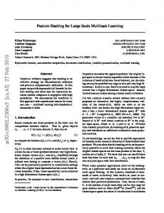
Data in Task 1 Data in Task 2 True Boundaries

2

Data in Task 1 Data in Task 2 True Boundaries IL−SVM in Task 1 IL−SVM in Task 2 MTL−OC in Task 1 MTL−OC in Task 2

2 1.5

1

1

1 y

y

y

0.5

0

Data in Task 1 Data in Task 2 True Boundaries One−SVM

2

0

0 −0.5

−1

−1

−1 −1.5

−2 −2

−1

0 x

1

2

(a) Data and True Boundaries

Fig. 1.

−2 −2

−1.5

−1

−0.5

0 x

0.5

•

2

−2 −2

−1

0 x

1

2

(c) One–SVM

Toy example with two tasks demonstrates the proposed model.

in the related t-th task, as νt = ν |TN|t . So we can use a single global parameter ν to control the fraction of support vectors and outliers consistently.

In the following, we discuss the properties of our proposed MTL for one-class classification.

•

1.5

(b) IL–SVM vs. MTL–OC

V. D ISCUSSION

•

1

Connection to one-class ν-SVM The one-class ν-SVM [22], [24] is a special case of our proposed MTL model. Actually, when the number of tasks is one, the optimization in (2) is reduced to the one-class ν-SVM. In addition, if we set Cη = 0, i.e., we discard the control of the closeness of the weights in related tasks, then our MTL framework for one-class classification corresponds to training each individual one-class ν-SVM. Relation to MTL via Conic Programming Our proposed MTL model focuses on the problem of one-class classification. When it employs the label information in a binary classification paradigm, it can be considered as a ν trick of the MTL via conic programming, which distinguishes itself from the formulation in [15]. Proposition of νs Similar to the property in one-class ν-SVM [24], we have the following proposition: Proposition 2: Suppose the solution of (2) satisfies ρt 6= 0 for the t-th task. The following statements hold: 1) νt is an upper bound on the fraction of outliers for the t-th task. 2) νt is a lower bound on the fraction of support vectors for the t-th task. 3) Suppose the data of the t-th task were generated independently from a distribution P (x) without discrete components and the kernel is analytic and non-constant. With probability 1, asymptotically, νt equals both the fraction of support vectors and outliers for the t-th task. The above proposition can be proved based on the constraints of the dual problem and the fact that outliers must have Lagrange multipliers at the upper bound. For practical applications, we can use a global ν, where νt is proportional to the number of the training samples

VI. E XPERIMENTS In this section, we demonstrate the validity and advantage of the proposed method through experiments.

A. Models and Measurement In the experiment, we compare three methods: our proposed MTL–OC model; individually learned SVM (IL– SVM) and One–SVM. For the MTL–OC model, data for all tasks and the information of their tasks relationships are fed into the model to get the boundaries for different tasks. For IL–SVM, data for each individual task are trained in a one-class ν-SVM individually. The decision boundary for each task is obtained correspondingly. For the One–SVM, all samples in the multiple tasks are considered as one big task and they are trained by the one-class ν-SVM. For all three models, the gaussian kernel, k(x, y) = exp(−γkx − yk2 ), is used as the feature kernel. The corresponding parameters are expressed in detail in the following subsection. For real-world datasets, the values of the parameters Cη and ν T for the MTL–OC model and related parameters for IL–SVM and One–SVM are tuned by crossvalidation over the training set. A good one-class classifier will try to minimize two types of errors, namely the fraction of false positives (FP) and the fraction of false negatives (FN). For a classifier, by varying the threshold, these two errors can be obtained correspondingly, and a Receiver Operating Characteristics (ROC) curve [20] is then obtained. Usually, the area under the ROC curve, AUC, can be used to measure the performance of a one-class classifier [8]. The larger the AUC, the better the one-class classifier. In the experiment, the AUC of the ROC is calculated by the trapezoid area.

2823

B. USPS Dataset 1

The U.S. Postal Service (USPS) database is a handwritten digits database containing 9298 digit images of size 16 × 16 = 256 pixels, of which the last 2007 comprise the test set. Pixel values in each image are scaled to the range of −1.0 and 1.0. Here, we create two fake but related tasks from this USPS database to mimic the application of recognizing some noisy images with the help of clear and related images. We choose digit ‘4’ as the target object and create two additional mask patterns with random noises which are generated from uniform distribution: one is with thin noise and the other one is with thick noise. We then add these two masks to the images of digit ‘4’ in the original training set of the USPS database. Figure 2 shows some samples of the final images on both the training and test datasets. The objective of this experiment is to show how clean data can be used for improving the performance of outlier detection on the noisy related data. In the training procedure, data in the created fake and related tasks are fed into the corresponding models to get the decision boundaries. The parameter, γ, of the feature 1 as in [22]. To test the effect of using kernel is set to 0.5·256 different numbers of training samples, we randomly select 5, 10, 20 and 40 samples from the training data for each task. In the test procedure, we only use the test set (2007 samples) of the USPS database and vary the threshold to get the corresponding ROC curve on the test set. We repeat the above procedure 20 times and average their AUCs. Table I reports the result on this task. Since there is only one test set for the target object, we average the AUCs of the IL–SVM and the MTL–OC as the final AUCs. It is obvious that our proposed MTL–OC model shows significant improvement over the IL–SVM and the One–SVM. For the IL– SVM, its performance reduces largely when training on the samples with thick noise. Moreover, its performance reduces as the number of training samples decreases for the thick noise case. This means that the more noise samples used in the training, the worse decision boundary may distract from the true one. On the contrary, our proposed MTL– OC can overcome the problem of the IL–SVM. Comparing our MTL–OC with the IL–SVM on the thick noise case, the performance of our model improves greatly. Overall, our model achieves the best performance in terms of the average AUCs. Although the performance of our MTL–OC training on the samples with thick noise does not beat that of the One–SVM on all samples, the corresponding performance of our MTL–OC is very close to that of the One–SVM and we achieve an overall better performance. Another observation is that as the number of training samples increases, the AUC increases correspondingly for the One–SVM and our MTL–OC. In the test, when the number of training samples increases from 20 to 40, there is no significant improvement on the performance. This means that when the number of 1 http://www-stat.stanford.edu/˜tibs/ ElemStatLearn/data.html

training samples achieves a certain value, it will not improve the performance for our MTL–OC. This experiment also gives us an illumination of how to detect outliers when the given one-class samples are noisy. For that case, we may try to collect some clean data and incorporate them in the training procedure to improve the detecting performance. C. Protein Super-Family Dataset In the following, we test the one-class classification on a real-world protein super-family dataset [1]. Table II gives a structural view of the dataset and the task relationships performed in the experiments. We will interpret it in the following. The data from the SCOP database is the same as that of [15]: 20 kinds of amino acids consist of 400 features. In this dataset, there are four super-classes which are termed as folds [15]: DNA/RNA binding fold, Flavodoxin fold, OB-fold and SH3 fold. Each fold is divided into several super-families [15]. The DNA/RNA binding fold contains three super-families and we denote them as d1, d2 and d3, respectively. The Flavodoxin fold contains four superfamilies and we denote them as f1, f2, f3, and f4, respectively. The OB-fold contains three super-families and we denote them as o1, o2 and o3, respectively. There are two superfamilies in the SH3 fold and are denoted as s1 and s2, respectively. The tasks’ relationships are constructed as follows: classifying a super-family is considered as one task for the oneclass classification. If two one-class classification tasks are in the same fold, we set them as related tasks and connect them by an edge. For an isolated task without any edge connection, our formulation of MTL–OC will define it as an independent task and its solution is consistent with that solved by the IL– SVM. Hence, we can perform the experiments on each fold respectively. The effect of the number of training samples is also tested on this dataset. We randomly choose N samples, where N equals 5, 10, and 20, from each super-family, in training for each task. The parameter of the feature kernel, γ = 2σ1 2 , where σ 2 is set to the average of the squared distances to the fifth nearest neighbors, as [15]. We then train on these samples to obtain the corresponding decision boundaries for all three models and calculate their AUCs correspondingly. The above procedure is repeated ten times and we average the results of the AUCs. The average results are shown in Fig. 3 and Fig. 4. From the results, we clearly see that the MTL–OC outperforms the IL–SVM and One–SVM mothods. It is interesting to note that the results of One–SVM are substantially worse than those of the IL–SVM. An exception exists for the subtask of the super-family f1. We guess this may be due to the skewness of the data. It is also noted that the AUCs are very small for the Flavonoid fold in all three models. Through experimental observations, there are very high false positive errors for three models in this fold. Overall, this dataset again demonstrates the advantage of our proposed MTL–OC model.

2824

(a) Training Samples

(b) Test Samples

Fig. 2.

Samples in the USPS dataset. TABLE I

T HE PERFORMANCE (AUC) OF EACH METHOD FOR THE USPS DATASET (%).

# 5 10 20 40

thin 82.2±5.1 86.2±2.7 87.2±1.9 87.3±1.3

IL–SVM thick 57.6±3.1 56.3±2.3 55.7±2.1 53.8±1.5

One–SVM average 81.7±5.1 82.8±2.9 83.3±1.2 84.1±1.1

average 69.9±3.9 71.2±2.3 71.4±1.8 70.5±1.2

thin 83.9±5.1 86.2±2.9 87.2±1.3 87.2±1.1

MTL–OC thick 81.2±5.2 82.8±2.4 83.1±1.6 83.1±1.5

average 82.6±5.2 84.5±2.6 85.1±1.4 85.2±1.3

TABLE II D ESCRIPTION OF THE PROTEIN SUPER - FAMILY DATASET.

Item Folds Super -families

Content Flavodoxin

DNA/RNA d1

d2

d3

f1

f2

f3

f4

OB o1

o2

SH3 o3

s1

s2

IL–SVM One–SVM MTL–OC

VII. C ONCLUSION AND F UTURE W ORK In this paper, we have proposed a new multi-task learning framework for one-class classification. The framework is to extend the one-class ν-SVM and to bound the distance between solutions of the related paired-tasks. The formulation is cast into a second-order cone program and is solved efficiently with a global optimal solution. We also demonstrated the advantage of our proposed model in the experiments on toy data, USPS digit data and a protein superfamily dataset. There are still several promising directions on the work. 1) Our framework is derived from the ν-SVM. It is interesting to derive a similar framework from the support vector domain description. 2) Our method exploits the information from related task through model structure assumption, but there are still other methods making use of the information inherent in multi-tasks through other kinds of knowledge, e. g., common features. How to utilize other kinds of inherent knowledge in related tasks is also an interesting

problem. 3) The effectiveness of our model has been demonstrated through experimental comparison. It is important and valuable to derive a framework to provide more theoretical justification of our model, e.g., analyzing the generalization error bound of the one-class classification in the MTL framework. 4) Now we have used standard toolboxes with standard methods, interior point method, to solve the SOCP problem. Standard methods contain the problem of scalability. Based on the specific form of our formulation, we believe there are still other methods to speed up the procedure of solving SOCP problem. How to speed it up and extend the scalability of our model is a promising research problem. ACKNOWLEDGMENTS The work described in this paper was substantially supported by two grants from the Research Grants Council of the Hong Kong SAR, China (Project No. CUHK4128/08E

2825

d2

58

82 IL−SVM One−SVM MTL−OC 10 # training samples

20

55 5

60

AUC (%)

54

AUC (%)

65

53

IL−SVM One−SVM MTL−OC 10 # training samples

20

50 5

50

10 # training samples

40 5

20

10 # training samples

20

(f) o3

f2

f3 28 26

20

20

10 5

(a) f1

10 # training samples

22 20 5

20

(b) f2

f4

63

AUC (%)

IL−SVM One−SVM MTL−OC

82

25 10 # training samples

(d) f4

20

80 5

10 # training samples

(e) s1

20

AUC (%)

62.5

84

30

20

s2

86 IL−SVM One−SVM MTL−OC

10 # training samples

(c) f3

s1

40

IL−SVM One−SVM MTL−OC

24

IL−SVM One−SVM MTL−OC

15

10 # training samples

AUC (%)

IL−SVM One−SVM MTL−OC

Fig. 4.

IL−SVM One−SVM MTL−OC

45

AUC (%)

AUC (%)

IL−SVM One−SVM MTL−OC

25

48.5

AUC (%)

o3

The performance (AUC) of each method on the d1, d2, d3, o1, o2, o3 data of the protein super-family dataset (%).

49

20 5

20

55

51

f1

35

10 # training samples

(c) d3

(e) o2

50

48 5

64 5

20

52

(d) o1

Fig. 3.

IL−SVM One−SVM MTL−OC

65

o2 55

50

10 # training samples

66

AUC (%)

o1

55

IL−SVM One−SVM MTL−OC

(b) d2

70

49.5

67

56

(a) d1

45 5

68

57

80 78 5

d3 69

AUC (%)

84

AUC (%)

59

AUC (%)

d1 86

62 IL−SVM One−SVM MTL−OC

61.5 61 5

10 # training samples

(f) s2

The performance (AUC) of each method on the f1, f2, f3, f4, s1, s2 data of the protein super-family dataset (%).

2826

20

and Project No. CUHK4154/09E). R EFERENCES [1] A. A., H. D., B. S.E., H. T.J.P., C. C., and M. A.G. Scop database in 2004: refinements integrate structure and sequence family data. Nucl. Acid Res., 32:D226–D229, 2004. [2] A. Argyriou, T. Evgeniou, and M. Pontil. Multi-task feature learning. In B. Sch¨olkopf, J. C. Platt, and T. Hoffman, editors, Advances in Neural Information Processing Systems 19, pages 41–48, 2006. [3] A. Argyriou, T. Evgeniou, and M. Pontil. Convex multi-task feature learning. Machine Learning, 73(3):243–272, 2008. [4] A. Argyriou, C. A. Micchelli, M. Pontil, and Y. Ying. A spectral regularization framework for multi-task structure learning. In J. Platt, D. Koller, Y. Singer, and S. Roweis, editors, Advances in Neural Information Processing Systems 20, pages 25–32. MIT Press, Cambridge, MA, 2008. [5] J. Baxter. A model of inductive bias learning. Journal of Artificial Intelligence Research, 12:149–198, 2000. [6] C. Bishop. Novelty detection and neural network validation. In IEE Proceedings on Vision, Image and Signal processing, Special issue on applications of neural networks, pages 141(4):217–222, 1994. [7] S. Boyd and L. Vandenberghe. Convex Optimization. Cambridge University Press, 2004. [8] A. Bradley. The use of the area under the ROC curve in the evaluation of machine learning algorithm. Pattern Recognition, 30(7):1145–1159, 1997. [9] R. Caruana. Multitask learning. Machine Learning, 28(1):41–75, 1997. [10] T. Evgeniou, C. A. Micchelli, and M. Pontil. Learning multiple tasks with kernel methods. Journal of Machine Learning Research, 6:615– 637, 2005. [11] T. Evgeniou and M. Pontil. Regularized multi–task learning. In W. Kim, R. Kohavi, J. Gehrke, and W. DuMouchel, editors, Proceedings of the Tenth ACM SIGKDD International Conference on Knowledge Discovery and Data Mining, pages 109–117, 2004. [12] D. Haussler. Convolution kernels on discrete structures. Technical report, UC Santa Cruz, 1999. [13] L. Jacob, F. Bach, and J.-P. Vert. Clustered multi-task learning: A convex formulation. In D. Koller, D. Schuurmans, Y. Bengio, and L. Bottou, editors, Advances in Neural Information Processing Systems 21, pages 745–752, 2008.

[14] T. Jebara. Multi-task feature and kernel selection for svms. In L. D. Raedt and S. Wrobel, editors, Proceedings of the Twenty-first International Conference, 2004. [15] T. Kato, H. Kashima, M. Sugiyama, and K. Asai. Multi-task learning via conic programming. In J. Platt, D. Koller, Y. Singer, and S. Roweis, editors, Advances in Neural Information Processing Systems 20, pages 737–744. MIT Press, Cambridge, MA, 2008. [16] L. Liang and V. Cherkassky. Connection between svm+ and multi-task learning. In IJCNN, pages 2048–2054, 2008. [17] J. Liu, S. Ji, and J. Ye. Multi-task feature learning via efficient l2,1 norm minimization. In UAI, 2009. [18] Q. Liu, X. Liao, and L. Carin. Semi-supervised multitask learning. In J. Platt, D. Koller, Y. Singer, and S. Roweis, editors, Advances in Neural Information Processing Systems 20, pages 937–944. MIT Press, Cambridge, MA, 2008. [19] M. Lobo, L. Vandenberghe, S. Boyd, and H. Lebret. Applications of second-order cone programming. Linear Algebra and its Applications, 284:193–228, 1998. [20] M. A. Maloof. On machine learning, ROC analysis, and statistical tests of significance. In Proceedings of the Sixteenth International Conference on Pattern Recognition (ICPR-2002), pages 204–207, Los Alamitos, CA, 2002. IEEE Press. [21] G. Obozinski, B. Taskar, and M. I. Jordan. Joint covariate selection and joint subspace selection for multiple classification problems. Statistics and Computing, 2009. [22] B. Sch¨olkopf, J. C. Platt, J. Shawe-Taylor, A. J. Smola, and R. C. Williamson. Estimating the support of a high-dimensional distribution. Neural Computation, 13(7):1443–1471, 2001. [23] B. Sch¨olkopf and A. Smola. Learning with Kernels. MIT Press, Cambridge, MA, 2002. [24] B. Sch¨olkopf, R. C. Williamson, A. J. Smola, J. Shawe-Taylor, and J. C. Platt. Support vector method for novelty detection. In NIPS, pages 582–588, 1999. [25] D. M. J. Tax and R. P. W. Duin. Support vector domain description. Pattern Recognition Letters, 20(11-13):1191–1199, 1999. [26] K. Tsuda and W. S. Noble. Learning kernels from biological networks by maximizing entropy. In ISMB/ECCB (Supplement of Bioinformatics), pages 326–333, 2004. [27] V. Vapnik. The Nature of Statistical Learning Theory. Springer, New York, 2nd edition, 1999.

2827