Multi-timescale Nexting in a Reinforcement ... - Semantic Scholar

Adaptive Behavior ():–

Multi-timescale Nexting in a Reinforcement Learning Robot

c

The Author(s) 2014 Reprints and permission: sagepub.co.uk/journalsPermissions.nav

Joseph Modayil, Adam White, and Richard S. Sutton Reinforcement Learning and Artificial Intelligence Laboratory University of Alberta, Edmonton, Alberta, Canada Abstract The term “nexting” has been used by psychologists to refer to the propensity of people and many other animals to continually predict what will happen next in an immediate, local, and personal sense. The ability to “next” constitutes a basic kind of awareness and knowledge of one’s environment. In this paper we present results with a robot that learns to next in real time, making thousands of predictions about sensory input signals at timescales from 0.1 to 8 seconds. Our predictions are formulated as a generalization of the value functions commonly used in reinforcement learning, where now an arbitrary function of the sensory input signals is used as a pseudo reward, and the discount rate determines the timescale. We show that six thousand predictions, each computed as a function of six thousand features of the state, can be learned and updated online ten times per second on a laptop computer, using the standard TD(λ) algorithm with linear function approximation. This approach is sufficiently computationally efficient to be used for real-time learning on the robot and sufficiently data efficient to achieve substantial accuracy within 30 minutes. Moreover, a single tile-coded feature representation suffices to accurately predict many different signals over a significant range of timescales. We also extend nexting beyond simple timescales by letting the discount rate be a function of the state and show that nexting predictions of this more general form can also be learned with substantial accuracy. General nexting provides a simple yet powerful mechanism for a robot to acquire predictive knowledge of the dynamics of its environment.

1. Multi-timescale Nexting Psychologists have noted that people and other animals seem to continually make large numbers of short-term predictions about their sensory input (Gilbert 2006, Brogden 1939, Pezzulo 2008, Carlsson et al. 2000). When we hear a melody we predict what the next note will be or when the next downbeat will occur, and we are surprised and interested (or annoyed) when our predictions are disconfirmed (Huron 2006, Levitin 2006). When we see a bird in flight, hear our own footsteps, or handle an object, we continually make and confirm multiple predictions about our sensory

input. When we ride a bike, ski, or rollerblade, we have finely tuned moment-by-moment predictions of whether we will fall and of how our trajectory will change in a turn. In all these examples, we continually predict what will happen to us next. Making predictions of this simple, personal, short-term kind has been called nexting (Gilbert 2006). Nexting predictions are specific to one individual and to their personal, immediate sensory signals or state variables. A special name for these predictions seems appropriate because they are unlike predictions of the stock market, of political events, or of fashion trends. Predictions of such

2

Adaptive Behavior () (a) Acceleration

(b) Motor current

causes limb retraction. The phenomenon is that after a while the limb starts to be retracted early, in response to the bell. This is interpreted as the bell causing a prediction of the shock, which then triggers limb retraction. In other experiments, for example those known as sensory preconditioning

Seconds

(c) Infrared distance

Seconds

(d) Light

(Brogden 1939, Rescorla 1980), it has been shown that animals learn predictive relationships between stimuli even when none of them are inherently good or bad (like food and shock) or connected to an innate response. In this case the predictions are made continually, but not expressed in behavior until some later experimental manipulation connects them to a response. Animals seem to be wired to learn

Seconds

Seconds

Fig. 1. Examples of sensory signals varying over very different time scales on the robot: (a) acceleration varying over tenths of a second, (b) motor current varying over fractions of a second, (c) infrared distance varying over seconds, and (d) ambient light varying over tens of seconds. The ranges of the sensor readings vary across the different sensor types.

the many predictive relationships in their world. To be able to next is to have a basic kind of knowledge about how the world works in interaction with one’s body. It is to have a limited form of forward model of the world’s dynamics. To be able to learn to next—to notice any disconfirmed predictions and continually adjust your nexting predictions—is to be aware of one’s world in a significant

public events seem to involve more cognition and deliberation, and are fewer in number. In nexting, we envision that one individual may be continually making massive numbers of small predictions in parallel. Moreover, nexting predictions seem to be made simultaneously at multiple time scales. When we read, for example, it seems likely that we next at the letter, word, and sentence levels, each involving substantially different time scales. In a similar fashion to these regularities in a person’s experience, our robot has predictable regularities at time scales ranging from tenths of seconds to tens of seconds (Figure 1). The ability to predict and anticipate has often been proposed as a key part of intelligence (e.g., Tolman 1951, Hawkins & Blakeslee 2004, Butz, Sigaud & G´erard 2003, Wolpert, Ghahramani & Jordan 1995, Clark 2013). Nexting can be seen as the most basic kind of prediction, preceding and possibly underlying all the others. That people and a wide variety of animals learn and make simple predictions at a range of short time scales is the standard modern interpretation of the basic learning phenomenon known as classical conditioning (Rescorla 1980, Pavlov 1927). In a standard classical conditioning experiment, an animal is repeatedly given a sensory cue followed by a special stimulus that elicits a reflex response. For example, the sound of a bell might be followed by a shock to the paw, which

way. Thus, to build a robot that can do both of these things is a natural goal for artificial intelligence. Prior attempts to achieve artificial nexting can be grouped in two approaches. The first approach is to build a myopic forward model of the world’s dynamics, either in terms of differential equations or state-transition probabilities (e.g., Wolpert, Ghahramani & Jordan 1995, Grush 2004, Sutton 1990). In this approach a small number of carefully chosen predictions are made of selected state variables. The model is myopic in that the predictions are only short term, either infinitesimally short in the case of differential equations, or maximally short in the case of the one-step predictions of Markov models. In these ways, this approach has ended up in practice being very different from nexting. The second approach, which we follow here, is to use temporal-difference (TD) methods to learn long-term predictions directly. The prior work pursuing this approach has almost all been in simulation and has used table-lookup representations and a small number of predictions (e.g., Sutton 1995, Kaelbling 1993, Singh 1992, Sutton, Precup & Singh 1999, Dayan & Hinton 1993). Sutton et al. (2011) showed real-time learning of TD predictions on a robot, but did not demonstrate the ability to learn many predictions in real time or with a single feature representation.

3 The main contribution of this paper is a demonstration

where γ i ∈ [0, 1) is the discount rate for the ith prediction.

that many nexting predictions can be learned in real-time

The discount rate determines the timescale of the predic-

on a robot through the use of temporal difference methods.

tion: to obtain a timescale of T time steps, the discount rate

Our results show that learning thousands of predictions in

is set to γ i = 1 −

parallel is feasible using a single representation and a sin-

learning will recognize (1) as analogous to the definition of

gle set of learning parameters. The results also demonstrate

a state-value function. The prediction at time t is analogous to the approximated value of the state at time t, and Git is

that the predictions achieve substantial accuracy within 30

1 T

. Readers familiar with reinforcement

minutes. Moreover, we show how simple extensions to the standard algorithm can express substantially more general

analogous to the “return at time t” in reinforcement learning

forms of prediction, and predictions of this more general

prediction at time t, and we refer to it as the ideal predic-

form can also be learned both accurately and quickly.

tion. In our main experimental results, the pseudo reward

terminology. In this paper, Git is the ideal value for the ith

was either a raw sensory signal or else a component of a state-feature vector (which we will introduce shortly), and the discount rate was one of four fixed values, γ i = 0, 0.8,

2. Nexting as Multiple Value Functions

0.95, or 0.9875, corresponding to timescales (T values) of

We take a reinforcement-learning approach to achieving

0.1, 0.5, 2, or 8 seconds.

nexting. In reinforcement learning it is commonplace to use

We use linear function approximation to form each pre-

TD methods such as the TD(λ) algorithm (Sutton 1988) to

diction. That is, we assume that the state of the world at

learn long-term predictions of reward, called value functions. The TD(λ) algorithm has also been used as a model of

time t is characterized by a feature vector φt ∈ t θt =

can be seen as taking this approach to the extreme, using

n X

φt (j)θti (j),

(2)

j=1

TD(λ) to predict massive numbers of a great variety of reward-like signals at many time scales (cf. Sutton 1995,

where φ> t denotes the transpose of φt (all vectors are col-

Sutton & Tanner 2005, Sutton et al. 2011).

umn vectors unless transposed) and φt (j) denotes its jth

We use a notation for our multiple predictions that

component. In our experiments the feature vectors had n =

mirrors—or rather multiplies—that used for conventional

6065 components, but only a fraction of them were nonzero,

value functions. Time is taken to be discrete, t = 1, 2, 3, . . .,

so the sums could be very cheaply computed.

with each time step corresponding to 0.1 seconds of real

The predictions at each time are determined by the

time. In conventional reinforcement learning, a single pre-

weight vectors θti . One natural and computationally frugal

diction is learned about a special signal called the “reward”

algorithm for learning the weight vectors is linear TD(λ),

and whose value at time t may be denoted Rt ∈ t θ − Gt


2

3. Scaling Experiment We explored the practicality of applying computational nexting as described above to make and learn thousands of

.

(5)

t=1

predictions, from thousands of features, in real time. We used a small mobile robot platform custom designed in our

The best static weight vector can be computed offline by

laboratory (Figure 2, left). The robot’s primary actuators

standard algorithms for solving large least-squares regres-

were three wheels placed in a standard omni-drive con-

2

sion problems. The standard algorithm is O(n ) in memory 3

2

figuration enabling it to rotate and move in any direction.

and either O(n ) or O(N n ) in computation, per predic-

Sensors attached to the motors reported the electrical cur-

tion, and is just barely tractable for offline use at the scale

rent, voltage, motor temperature, wheel rotational velocity,

we consider here (in which n = 6065). Although this algo-

and an overheating flag, providing substantial observability

rithm is not practical for online use, its solution

θ∗i

provides

of the internal physical state of the robot. Other sensors col-

a useful performance standard. Note that even the best static

lected information from the external environment. Passive

weight vector will incur some error. It is even theoretically possible that an online learning algorithm could perform

sensors detected ambient light in several directions in the visible and infrared spectrum. Active sensors on the sides

better than θ∗i , by adapting to gradual changes in the world

of the robot emitted infrared (IR) light and measured the

or robot. But under normal circumstances an online learn-

amount of reflected IR light, providing information about

ing algorithm will only hope to approach the performance of the best static weight vector in the limit of infinite data.

the distance to nearby obstacles. Other sensors measured

Note that in presenting algorithms in this section we have

the state of the robot was characterized by 53 real or virtual

carefully avoided any mention of expectations or states. We

sensors of 13 types, as summarized in the first two columns

acceleration, rotation, and the magnetic field. All together,

of Table 1.

5 Sensor type IRdistance

Num of sensors 10

Light

4

IRlight

8

Thermal RotationalVelocity Magnetic Acceleration MotorSpeed

4(8) 1 3 3 3

MotorVoltage MotorCurrent MotorTemperature LastMotorRequest OverheatingFlag

3 3 3 3 1

tiling type 1D 1D 2D 2D+1 1D 2D 1D 1D 2D 2D+1 1D 1D 1D 1D 1D 2D 1D 1D 1D 1D 1D

Num of intervals 8 2 4 4 4 4 8 4 8 8 8 8 8 8 8 8 8 8 4 6 2

Num of tilings 8 4 4 4 8 1 6 1 1 1 4 8 8 8 4 8 2 2 4 4 4

Table 1. Summary of the tile-coding strategy used to produce feature vectors from sensory signals. For each sensor of a given type, its tilings were either 1-dimensional or 2-dimensional, with the given number of intervals (see text and Figure 3). Only the first four of the robot’s eight thermal sensors were included in the tile coding due to a coding error.

The robot’s interaction with its environment was structured in a tight loop with a 100 millisecond (ms) time step. At each step, the sensory information was used to select one of seven actions corresponding to basic movements of the robot (forward, backward, slide right, slide left, turn right, turn left, and stop). Each action caused a different set of voltage commands to be sent to the three motors driving the wheels. The experiment was conducted in a square wooden pen, approximately two meters on a side, with a lamp on one edge (Figure 2, right). The robot selected actions according to a fixed stochastic policy that caused it to generally follow a wall on its right side. The policy selected the forward action by default, the slide-left or slide-right action when the right-side-facing IR distance sensor exceeded or fell below given thresholds, and selected the backward action when the front IR distance sensor exceeded another threshold (indicating an obstacle ahead). We chose the thresholds such that the robot rarely collided with the wall and rarely strayed more than half a meter from the wall. By design, the backward action also caused the robot to turn slightly

to the left, facilitating the many left turns needed for wall following on the right. To inject some variability into the behavior, on 5% of the time steps the policy instead chose an action at random from the seven possibilities with equal probability. Following this policy, the robot usually completed a circuit of the pen in about 40 seconds. A circuit took significantly longer if the motors overheated and temporarily shut themselves down. In this case the robot did not move, irrespective of the action chosen by the policy. Shut downs occurred approximately every 8 minutes and lasted for about 7 minutes. This simple policy was sufficient for the robot to reliably follow the wall for hours. To produce the feature vectors needed for the TD(λ) algorithm, the sensor readings were coarsely coded as 6065 binary features according to a tile-coding strategy as summarized in Table 1 and exemplified in Figure 3. Tile coding is a standard technique for converting continuous variables into a sparse feature representation that is well suited for online learning algorithms. The sensor readings are taken in small groups and partitioned, or tiled, into non-overlapping regions called tiles. One such tiling over two sensor readings from our robot is shown on the left side of Figure 3. In this case the tiling is a simple regular grid of square tiles of equal width (for some other possibilities see Sutton & Barto 1998, p. 206-7). Tile coding becomes much more powerful than a simple discretizing of the state space through the use of multiple overlapping tilings that are offset from each other as shown in the right side of Figure 3. For each tiling, a given state (e.g., the state marked by a white dot in the figure) is in exactly one tile. The set of tiles that are activated by a state constitute a coarse coding of the state’s location in sensor space. The resolution of this coding is finer than that of the individual tilings, as suggested by the greater density of lines in Figure 3 (right). With four tilings, the effective resolution is roughly four times that of the original tiling. The advantage of the multiple tilings over a single tiling with four times the resolution is that generalization will be broader with multiple tilings, which typically leads to much faster learning. With tile coding one can quickly learn a coarse approximation to the desired mapping, and then refine it with further data, simultaneously obtaining the benefits of both coarse and fine discretizations.

6

Adaptive Behavior ()

Number of intervals = 4 Tiling 1 Tiling 2 Tiling 3 Tiling 4

IR distance sensor3

255

0

Continuous 2D sensor space 0

IR distance sensor1

255

Sensor reading input

Four active tiles output

Fig. 3. An example of how tile coding was used to map continuous sensor input into many binary features. On the left we see a single tiling of the continuous 2D space corresponding to the readings from two non-consecutive (2D+1) IR distance sensors. The space was tiled into 4 intervals in each dimension, for 16 tiles overall. On the right we see all four tilings, each offset by a different negative amount such that they were equally spaced, with the first tiling starting at the lower left of the sensor space (as shown on the left) and the last tiling ending at the upper right of the space. A sensor reading input to the tile coder is a point in the space, like that shown by the white dot. The output of tile coding is the indices of the four tiles that contain the point, as shown on the right. These tiles are said to be active, and their corresponding features take on the value 1, while all the non-active tiles correspond to features with the value 0. Note how the four tilings provide a dense grid of lines, each a distinction that can be made between input points, yet the four active tiles together span a substantial portion of the sensor space. In this way, multiple tilings provides a feature representation that enables both fine resolution and broad generalization. This tile-coding example corresponds to the fourth row of Table 1.

Each tile in a tiling corresponds to a single binary fea-

We first applied TD(λ) to make and learn 2160 predic-

ture. If the current sensor readings fall in that tile, then

tions. The pseudo-reward signals Rti of the predictions were

the feature is active and takes the value 1, otherwise it is

the 53 sensor readings and a random selection of 487 from

inactive and takes the value 0. In our representation, we

the 6064 non-bias features. For each of these signals, four

had n = 6065 such features making up our binary fea-

predictions were learned with the four values of the dis-

6065

. The specifics of our tile-

count rate, γ i = 0, 0.8, 0.95, and 0.9875, corresponding to

coding strategy are summarized in Table 1. Most of our

timescales of 0.1, 0.5, 2, and 8 seconds respectively. Thus,

tilings were 1-dimensional (1D), that is, over a single sen-

we sought to learn a total of (53 + 487) × 4 = 2160 predic-

sor reading, in which case a tile was simply an interval of

tions. The learning parameters were λ = 0.9 and α =

the sensor reading’s value. For some sensors we formed

(as there are 457 active features), and the initial weight vec-

2-dimensional (2D) tilings by taking neighboring sensors in pairs. This enabled the robot’s features to distinguish

tor was zero. Data was logged to disk for later analysis. The total run time for this experiment was approximately three

between, for example, a wall and a corner. To provide fur-

hours and twenty minutes (120,000 time steps).

ture vectors, φt ∈ {0, 1}

0.1 457

ther discriminatory power, for some sensor types we also

We can now address the main question: is real-time nex-

formed 2-dimensional tilings from pairs consisting of a sen-

ting practical at this scale? In our setup, this comes down to

sor and its second-neighboring sensor. These are indicated as 2D+1 tilings in Table 1 (and this is the specific case illus-

whether or not all the computations for making and learn-

trated in Figure 3). Finally, we added a tiling with a single

within the robot’s 100ms time step. The wall-following pol-

tile that covered the entire sensor space and thus whose

icy, tile-coding, and TD(λ) were all implemented in Java

corresponding feature, called the bias feature, was always

and run on a laptop computer connected to the robot by a

active. Altogether, our tile-coding strategy used 457 tilings,

dedicated wireless link. The laptop used an Intel Core 2 Duo

producing feature vectors with n = 6065 components, most

processor with a 2.4GHz clock cycle, 3MB of shared L3

of which were zeros, but exactly 457 of which were ones.

ing so many complex predictions can be reliably completed

7 cache, and 4GB DDR3 RAM. The system garbage collec-

60,000

tor was called on every time step to reduce variability. Four

Ideal 8s Light3 prediction

threads were used for the learning code. The total memory consumption was 400MB. With this setup, the time required

40,000

(right scale)

(left scale)

to make and update all 2160 predictions was 55ms, well within the 100ms duty cycle of the robot. This demonstrates

1024 1024

Light3 pseudo reward

512 20,000

that it is indeed practical to do large-scale nexting on a robot with conventional computational resources. Later, on a newer laptop computer (Intel Core i7, 2.7 Ghz quad core, 8GB 1600 Mhz DDR3 RAM, 8 threads), with the

0,000

0

40

60

60,000

same style of predictions and the same features, we found

TD(λ) prediction

that we were able to make 6000 predictions in 85ms. This shows that with more computational resources, the num-

20

40,000

ber of predictions (or the size of the feature vectors) can

80

100

0 120

Prediction of best static θ Ideal 8s Light3 prediction

be increased proportionally. This strategy for nexting easily scales to millions of predictions with foreseeable increases

20,000

in computing power over the next decade. 0

0

20

40

60

80

100

120

Seconds

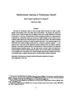
4. Accuracy of Learned Predictions The predictions were learned with substantial accuracy. For example, consider the eight-second prediction whose pseudo reward is the third light-sensor reading (Light3). Notice that there is a bright lamp in the lower-left corner of the pen (Figure 2, right). On each trip around the pen, the reading from this light sensor increased to its maximal level and then fell back to a low level, as shown in the upper por-

Fig. 4. Predictions of the Light3 pseudo reward at the eightsecond timescale. The upper graph shows the Light3 sensor reading spiking and saturating on three circuits around the pen and the corresponding ideal prediction (computed afterwards from the future pseudo rewards). Note that the ideal prediction shows the signature of nexting—a substantial increase prior to the spikes in pseudo reward. The lower graph shows the same ideal prediction compared to the prediction of the TD(λ) algorithm and of the prediction of the best static weight vector. These feature-based predictions are more variable, but substantially track the ideal.

tion of Figure 4. If the state features are sufficiently informative, then the robot should be able to anticipate the rising and falling of this sensor reading. Also shown in the figure

60,000

is the ideal prediction for this time series, Git , computed retrospectively from the subsequent readings of the light sensor. Of course no real predictor could achieve this—our learning algorithms seek to approximate this ‘clairvoyant’ prediction using only the sensory information available in the current feature vector.

Ideal 8s Light3 prediction

Average over 100 circuits around the pen

TD(") prediction Onset of Light3 saturation

The prediction made by TD(λ) is shown in the lower portion of Figure 4, along with the prediction made by the best static weight vector θ∗i computed retrospectively as

Prediction of best static !

0

15 seconds near the time of Light3 saturation

described in Section 2. The key result is that the TD(λ) prediction anticipates both the rise and fall of the light. Both the learned prediction and the best static prediction track the ideal prediction, though with visible fluctuations.

Fig. 5. Light3 predictions (like those in the lower portion of Figure 4) averaged over 100 circuits around the pen and aligned at the onset of Light3 saturation.

8

Adaptive Behavior () 40,000

MagneticX pseudo reward

TD(λ) prediction (left scale)

(right scale)

32,000

24,000

500

25,000

400

20,000

300

16,000

200

Ideal 8s prediction

Best constant

RMSE of 8s Light3 prediction

Autoregressive Bias

(left scale)

8,000

TD(1)

100

0

20

40

60

80

100

5,000

120

TD(") TD(0) Best static !

Seconds

0

Fig. 6. Predictions of the MagneticX sensor at the eight-second timescale. The TD(λ) prediction was close to the ideal prediction, explaining 90 percent of its variance.

To remove these fluctuations and highlight the general trends in the eight-second predictions of Light3, we averaged the predictions over 100 circuits around the pen, aligning each circuit’s data to the time of initial saturation of the light sensor. The average of the ideal, TD(λ), and beststatic-weight-vector predictions for 15 seconds near the

0

30

60

90

120

150

180

Minutes Fig. 7. Learning curves for 8-second Light3 predictions made by various algorithms over the full data set. Each point is the RMSE of the prediction of the algorithm up to that time. Most algorithms use only the data available up to that time, but the best-static-θ and best-constant algorithms use knowledge of the whole data set. The errors of all algorithms increased at about 130 and 150 minutes because the motors overheated and shutdown at those times while the robot was passing near the light, causing an unusual pattern of sensor readings. In spite of the unusual events, the RMSE of TD(λ) still approached that of the best static weight vector. See text for the other algorithms.

time of saturation are shown in Figure 5. All three averages rise in anticipation of the onset of Light3 saturation and fall rapidly afterwards. The ideal prediction peaks before

as:

elevated prior to saturation. The two learned predictions

v u T u1 X t RMSE(i, T ) = (V i − Git )2 . T t=1 t

are roughly similar to the ideal, and to each other, but

Figure 7 shows the RMSE of the eight-second Light3 pre-

there are substantial differences. These differences do not

dictions for various algorithms. For TD(λ), the parameters

necessarily indicate error or essential characteristics of the

were set as described above. For all the other algorithms,

algorithms. For example, such differences can arise because

their parameters were tuned manually to optimize the final

the average is over a biased sample of data—those time

RMSE. The other algorithms included TD(λ) for λ = 0

steps that preceded a large rise in the pseudo reward. We

and λ = 1, both of which performed slightly worse than λ = 0.9. Also shown is the RMSE of the prediction of the

saturation, because the Light3 reading regularly became

have established that some of the differences are due to the motor shutdowns. Notably, if the data from the shutdowns are excluded, then the prominent bump in the best-static-

best static weight vector and of the best constant predic-

θ prediction (in Figure 5) at the time of saturation onset

change over time, but the RMSE measure varies as harder

disappears.

or easier states from which to make predictions are encoun-

tion. In these cases the prediction function does not actually

Figure 6 shows another example of the accuracy of the

tered. Note that the RMSE of the TD(λ) prediction comes to

near-final TD(λ) predictions, in this case of one of the Mag-

closely approach that of the best static weight vector after

netometer sensor readings at an eight-second timescale.

about 90 minutes. This demonstrates that online learning

We turn now to consider how the quality of the eightsecond Light3 prediction evolves over time and data. As {Vti }

on robots can be effective in real time with a few hours of experience, even with a large state representation.

up

The benefits of a large representation are shown in Figure

through time T , we use the root mean squared error, defined

7 by the substantially improved performance over the ‘Bias’

a measure of the quality of a prediction sequence

9 2.0

1000

1.5

100

2s AccelY

Mean

Normalized MSE of TD(λ) 1.0 predictions (both graphs)

10

0.1s AccelX

0.5

1.0

Median

Mean w/ average subtracted 8s Light3

0.0

0

30

60

90

120

150

180

0.1

Minutes

0

30

60

90

120

150

180

Minutes

Fig. 8. Learning curves for the 212 predictions whose pseudo reward is a sensor reading. The median and several representative learning curves are shown on a linear scale on the left, and the mean learning curve is shown on a logarithmic scale on the right. The mean curve is high because of a minority of the sensors whose absolute values are high and whose variance is low. If the experiment is rerun using pseudo rewards with their average value subtracted out, then the mean performance is greatly improved, as shown on the right, explaining 78% of the variance in the ideal prediction by the end of the data set.

algorithm, which was TD(0) with a trivial representation

to one when the prediction is constant at the average ideal

consisting only of the bias feature (the single feature that

prediction.

is always 1). As an additional performance standard, also

Learning curves using the NMSE measure for the 212

shown is the RMSE of an autoregressive algorithm (e.g., see

predictions whose pseudo reward was a sensor reading are

Box, Jenkins & Reinsel 2011) that uses previous readings of

shown in Figure 8. The left panel shows the median learning

the Light3 sensor as features of a linear predictor, with the

curve and curves for a selection of individual predictions.

weights trained according to the least-mean-square rule. To

In most cases, the error decreased rapidly over time, falling

incrementally train the autoregressive model, the learning

substantially below the unit variance line. The median pre-

was delayed by 600 timesteps to compute the ideal predic-

diction explained 80% of the variance at the end of training

tion. The best performance of this algorithm was obtained

and 71% of the variance after just 30 minutes. In many

using a model of order 300, meaning the last 300 readings

cases the decrease in error was not monotonic, sometimes

of the Light3 sensor were used. The autoregressive model

rising sharply (presumably as a new part of the state space

performed much worse than all the algorithms that used a

was encountered) before falling further. In some cases, such

rich feature representation.

as the 2-second Y-acceleration prediction shown, the sensor was never effectively predicted, evidenced by its NMSE

Moving beyond the single prediction of one light sensor at one timescale, we next evaluate the accuracy of all 212 predictions about sensors at various timescales. To measure

never falling below one. We believe this signal was simply

the accuracy of predictions with different magnitudes, we

The mean learning curve, shown in the right panel of

unpredictable with the feature representation provided. Figure 8 on a log scale, fell rapidly but was always substan-

used a normalized mean squared error,

tially above one. This was due to a minority of the sensors

RMSE2 (i, t) , NMSE(i, t) = var(i)

(mainly the thermal sensors) whose values were far from zero but whose variance was small. The learning curves

in which the mean squared error is scaled by var(i), the Git

for the corresponding predictions were all very high (and

over all the

do not appear in the left panel because they were way off

timesteps. This error measure can be interpreted as the per-

the scale). Why did this happen? Note that our prediction

cent of variance not explained by the prediction. It is equal

algorithm was biased in that all the initial predictions were

sample variance of the ideal predictions

10

Adaptive Behavior ()

zero (because the weight vector was initialized to zero).

discount rate, γ i , has been varied only from prediction to

When the pseudo rewards are large relative to their vari-

prediction; for the ith prediction, γ i was constant and deter-

ance, this bias can result in a very large NMSE that takes

mined its timescale. Now we will allow the discount rate for

a long time to subside. One way to eliminate the bias is to

an individual prediction to vary over time depending on the

modify the pseudo rewards by subtracting from each sensor

state the robot finds itself in; we will denote its value at time

value the average of its values up to that time (e.g., the first

t as γti ∈ [0, 1]. With a constant discount rate, predictions

pseudo reward is always zero). This is easily computed and

are restricted to simple timescales in which pseudo rewards

uses only information readily available at the time. Most importantly, choosing the initial predictions to be zero is no

are weighted geometrically less the more they are delayed, as was given by the earlier definition of the ideal prediction:

longer a bias but simply the right choice. When we mod-

∞ X

Vti ≈

ified our pseudo rewards in this way, and reran TD(λ) on the logged data, we obtained the much lower mean learning curve shown in Figure 8 (right). In the mean, the prediction learned with the average subtracted explained 78% of the variance of the ideal prediction by the end of the data set.

def

i (γ i )k Rt+k+1 = Git .

(1)

k=0

With a variable discount rate, the weighting is not by simple powers of γ i , but by products of γti :

Finally, consider the majority of the predictions whose

Vti ≈

pseudo reward was one of the binary features making up the

∞ X


i def i Πkj=1 γt+j Rt+k+1 = Git .

(6)

k=0

feature vector. There were 170 constant features among the 487 binary features that were selected to be pseudo rewards,

The learning algorithm remains unchanged in form and

and thus with the average subtracted, both the ideal pre-

computational complexity; it is exactly as given earlier,

dictions and the learned predictions were constant at zero. For these constant predictions, the RMSE was zero and the variance was zero, and we excluded these predictions from

i , as appropriate: except with γ i replaced by γti or γt+1


i i i i i > i θt+1 = θti + α Rt+1 + γt+1 φ> t+1 θt − φt θt zt ,

further analysis. For the remainder of the predictions, both

i zti = γti λzt−1 + φt .

the median and mean explained 30% of the variance of the ideal prediction by the end of the data set.

(7) (8)

This small change results in a significant increase in the

These results provide evidence that real-time parallel

kinds of ideal predictions that can be expressed (Sutton

learning of thousands of accurate nexting predictions on a

1995, Maei & Sutton 2010, Sutton et al. 2011). Our con-

physical robot is possible and practical. Learning to sub-

tribution in this section is to apply and demonstrate this

stantial accuracy was achieved within 30 minutes of train-

generalization of TD(λ) in three examples of nexting in

ing, with no tuning of algorithm parameters, and using a single feature representation for all predictions. The par-

robots. For the first example, consider a discount rate that is usu-

allel scalability of knowledge-acquisition in this approach

ally constant and near one, but falls to zero when some

is substantially novel when compared with the predomi-

designated event occurs. In particular, consider

nately sequential existing approaches common for robot learning. Our results also show that online methods can be competitive in accuracy with an offline optimization method.

( γti

=

0

if Light3 is saturated at time t;

0.9875

otherwise.

As long as Light3 is not saturated, this discount rate works like an ordinary eight-second timescale—pseudo rewards are weighted by 0.9875 carried to the power of how many

5. Beyond Simple Timescales

steps they are delayed. But if Light3 ever becomes satu-

In this section we present a small generalization of the

rated, then all pseudo rewards after that time are given zero

TD(λ) algorithm that enables it to learn predictions of a sig-

weight. This kind of discount enables us to predict how

nificantly more general and expressive form. Up to now, the

11 to the pseudo reward; if signals are mixed into the pseudo

Times of Light3 saturation

300,000

TD(λ) prediction

reward in the right way, then predictions about the signals can be made with general temporal profiles. In particular,

200,000

it may be useful to predict what value a signal will have

Power-consumption pseudo reward (right scale)

0

at the time some event occurs. For example, suppose we

Ideal prediction of 8s power consumption until Light3 saturation

100,000

have some signal Xt whose value we wish to predict not in the short term, but rather at the time of some event. To do 5,000

this, we construct a discount rate γti that is one up until the event has occurred, then is zero. The pseudo reward is then

0

10

20

30

40

50

60

70

0 80

constructed as follows:

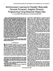
Seconds Fig. 9. Predictions of total power consumption, over an eightsecond time scale, or up until the Light3 sensor reading is saturated. To express this kind of prediction, the discount rate must vary with time (in this case dropping to zero upon Light3 saturation).

Rti = (1 − γti )Xt .

(9)

This pseudo reward is forced to be zero prior to the event (because 1 − γti is zero) and thus nothing that happens during this time can affect the ideal prediction. The ideal prediction will be exactly the value of Xt at the time γti first

much of something will occur prior to a designated event (in this case, prior to Light3 saturation). The pseudo reward in this example is a measure of the total power consumption of the three motors,

becomes zero. Constructing the pseudo reward by (9) has several possible interpretations depending on the exact form of Xt and γti . If Xt is the indicator function for an event (equal to one during it, zero otherwise), and γti is a constant less

Rti =

3 X

|MotorVoltagejt × MotorCurrentjt |.

j=1

than one prior to the event (and zero during the event), then the prediction will be of how imminent the onset of the event is. Figure 10 shows results with an example of

As shown in Figure 9, power consumption tended to vary

this using the data from our robot: γti prior to the event

between 1000 and 3000 depending on how many motors

was 0.8 (corresponding to a half-second timescale), and the

were active. The ideal prediction, also shown in Figure 9,

event was a right-facing IR sensor exceeding a threshold

was similar to that of an eight-second prediction for much

(corresponding to being within 12cm of the wall).

of the time, but notice how it falls all the way to zero during

Our final example, in Figure 11, illustrates the use of sig-

Light3 saturation. Even though there was substantial power

nals Xt that are not binary and discount rates γti that do not

consumption within the subsequent eight seconds, this has

fall all the way to zero. The idea here is to predict what the

no effect on the ideal prediction because of the saturation-

four light-sensor readings will be as the robot rounds the

triggered discounting. The figure shows that the modified

next corner of the pen. Four predictions are created, one for

TD(λ) algorithm performed well here (after training on the

each light sensor, with signals Xti = Lighti equal to the sensor reading. Rounding a corner is an event indicated by

previous 150 minutes of experience): over the entire data set the predictions captured approximately 88% of the variance in the ideal prediction.

a value from the side IR distance sensor corresponding to a large distance (>≈25cm). This typically occurs for sev-

The ideal prediction in the above example, like those of

eral seconds during the corner’s turn. We set the discount

simple timescales, always weights delayed pseudo rewards

rate γti equal to 0.9875 (an eight-second timescale) most of

less than immediate ones. It cannot put higher weight on the

the time, and equal to 0.3 when rounding a corner. Because

pseudo rewards received later than those received immedi-

the discount rate is greater than zero during the event, the

ately. This limitation is inherent in the definition of the ideal

light readings from several time steps contribute to the ideal

prediction (6) together with the restriction of the discount

prediction as the corner is entered.

rate to [0, 1]. However, it is only a limitation with respect

12

Adaptive Behavior ()

1.4

Times of closeto-wall events

1.2

1023

Light3

1.0 0 TD(λ) 1023 prediction of light sensors 0 1023 when entering next corner 0

0.8 0.6

TD(λ) prediction of event onset

0.4 0.2

Ideal prediction

0.0

Light1

1023

-0.2 -0.4

Light2

0

2

4

6

8

Light0

Ideal prediction

10 0

Seconds Fig. 10. Predictions of the imminence of the onset of an event regardless of its duration. The event here is being too close (