JMLR: Workshop and Conference Proceedings 80:1–16, 2017
ACML 2017
Multi-view Clustering with Adaptively Learned Graph Hong Tao Chenping Hou Jubo Zhu Dongyun Yi
[email protected] [email protected] ju bo
[email protected] [email protected] College of Science, National University of Defense Technology, Changsha, Hunan, 410073, China
Editors: Yung-Kyun Noh and Min-Ling Zhang
Abstract Multi-view clustering, which aims to improve the clustering performance by exploring the data’s multiple representations, has become an important research direction. Graph based methods have been widely studied and achieve promising performance for multi-view clustering. However, most existing multi-view graph based methods perform clustering on the fixed input graphs, and the results are dependent on the quality of input graphs. In this paper, instead of fixing the input graphs, we propose Multi-view clustering with Adaptively Learned Graph (MALG), learning a new common similarity matrix. In our model, we not only consider the importance of multiple graphs from view level, but also focus on the performance of similarities within a view from sample-pair level. Sample-pair-specific weights are introduced to exploit the connection across views in more depth. In addition, the obtained optimal graph can be partitioned into specific clusters directly, according to its connected components. Experimental results on toy and real-world datasets demonstrate the efficacy of the proposed algorithm. Keywords: Multi-view Clustering, Graph-based Learning, Sample Pair Significance
1. Introduction In many real-world applications, such as video surveillance and image retrieval, heterogeneous features can be obtained to represent the same instance. For example, an image can be characterized by various descriptors, such as SIFT (Lowe (2004)), histograms of oriented gradients (HOG) (Dalal and Triggs (2005)), GIST (Oliva and Torralba (2001)) and local binary pattern (LBP) (Ojala et al. (2002)); a webpage can be described by its content, the text of webpages linking to it, and the link structure of linked pages. Since these heterogeneous features summarize the objects’ characteristics from distinct perspectives, they are regarded as multiple views of the data. Multi-view learning, which explores the information from different views to improve the learning performance, has become an important research direction (Xu et al. (2013); Hou et al. (2017)). Clustering is the task to partition objects into meaningful groups without label information. To properly integrate the information from multiple views, many multi-view clustering approaches have been proposed (Chaudhuri et al. (2009); Kumar and Daum´e (2011); Liu et al. (2013); Cai et al. (2013)). Among these methods, a number of graph based multiview clustering algorithms were presented with good performance. Kumar et al. (2011) extended spectral clustering for multi-view learning by co-regularizing the clustering hyc 2017 H. Tao, C. Hou, J. Zhu & D. Yi. ⃝
Tao Hou Zhu Yi
potheses to make graphs from different views agree with each other. With a nonnegative constraint on the relaxed cluster assignment matrix, Cai et al. (2011) developed the multimodal spectral clustering (MMSC) algorithm to learn a commonly shared graph Laplacian matrix. Based on bipartite graph, Li et al. (2015) utilized local manifold fusion to integrate heterogeneous features and proposed a new large-scale multi-view spectral approach (MVSC). Nie et al. (2017) proposed a multi-view clustering method with adaptive neighbors (MLAN), this method performs clustering and local structure learning simultaneously. Despite the efficacy of graph based multi-view clustering methods, there still exists some limits. On one hand, some methods conduct the subsequent procedures based on the given similarity matrices without modifying them. Thus, the clustering results are dependent on the quality of the input graphs. To solve this problem, Nie et al. (2016) proposed a constrained laplacian rank (CLR) model to learn a new similarity matrix based on the given initial affinity matrix. By imposing rank constraint on the corresponding Laplacian matrix, the resultant similarity matrix has c exact connected components (c is the number of clusters) and each component corresponds to a cluster. However, CLR is developed in single-view setting and is inapplicable to dealing with multiple graphs simultaneously. On the other hand, those methods combining different views only consider the diversity of view contributions, but ignore the quality of pairwise relationships within the same view. In practice, the noise is usually non-homogeneously distributed, similarities of different sample pairs within the same view might also have varied capability for distinguishing the true cluster structure. Thus, sample pair significance analysis is very important for learning the detailed connection across views. Instead of treating similarities of different sample pairs equally (using the same weight for a certain view), a promising choice is to assume that different similarities usually have distinct weights according to their sample pair significance. Specifically, we introduce sample-pair-specific weights to measure the sample pair significance. How to adaptively learn these sample-pair-specific weights is crucial to find the right clustering structure. Self-paced learning (SPL) (Kumar et al. (2010); Jiang et al. (2014)), which incorporates samples from ‘easy’ to ‘complex’ into the training process by adaptively assigning them weights, offers a feasible strategy for addressing this problem. There are two weighting manners in SPL, i.e., hard weighting and soft weighting. Soft weighting is demonstrated more effective in previous studies (Xu et al. (2015); Zhao et al. (2015)) and also fits our setting better. Hence, we transplant the soft weighting manner of SPL into multi-view graph based clustering. In this paper, based on CLR, we propose Multi-view clustering with Adaptively Learned Graph (MALG), considering both ℓ1 -norm and ℓ2 -norm distances. Specifically, given initial affinity matrices from multiple views, we attempt to learn a new common similarity matrix with explicit clustering structure by forcing rank constraint on the corresponding Laplacian matrix. Meanwhile, both the quality diversity of multiple graphs and the sample pair significance within a certain graph are taken into consideration by introducing the sample-pair-specific weights. Based on the above two aspects, the resulting model is able to adaptively learn a new common similarity matrix and exploit the connection between different views in more depth. There are several benefits of our approach: The proposed approach modifying the similarity matrix during each iteration until reach to the optimal one, and the outputted similarity matrix explicitly give the clustering result; The sample-pair-specific weights are 2
Multi-view Clustering with Adaptively Learned Graph
first employed to measure the quality of similarities of different sample pairs for multi-view graph based clustering; The proposed objective functions can be solved by a simple yet effective algorithm; The clustering performance of the proposed method is examined on toy and real-world datasets and our approach outperforms other related methods in most cases.
2. Related Works We first introduce the notations used in this paper. Matrices and vectors are written as boldface uppercase letters and boldface lowercase letters respectively. For matrix M, the i-th row and the ij-th element of M are denoted as mi and mij , respectively. The trace of matrix M is denoted by T r(M). The transpose of matrix M is denoted as MT . The ℓ1 norm and ℓ2 -norm of vector v is denoted by ∥v∥1 and ∥v∥2 , the Frobenius and the ℓ1 -norm of matrix M are represented as ∥M∥F and ∥M∥1 respectively. 1 denotes a column vector with all ones, and the identity matrix is denoted by I. 2.1. CLR Revised Given an initial similarity matrix A ∈ Rn×n , CLR aims to learn a new similarity matrix S ∈ Rn×n with exact c connected components, where n is the number of data points and c is the T number of clusters. The Laplacian matrix related to S is defined ∑ as LS = DS − (S + S)/2, where DS is a diagonal matrix with i-th diagonal element as j (sij + sji )/2. There is an important property of the Lapalcian matrix as follows (Chung (1997)). Theorem 1 The multiplicity c of the eigenvalue 0 of the Laplacian matrix LS is equal to the number of connected components in the graph associated with S. Based on this observation, Nie et al. (2016) constrained the rank of LS to be n − c, and proposed the following CLR model for graph based clustering with both ℓ1 -norm and ℓ2 -norm distances: JCLR−ℓ1 = ∑ j
JCLR−ℓ2 = ∑
min
∥S − A∥1 ,
(1)
min
∥S − A∥2F .
(2)
sij =1,sij ≥0,rank(LS )=n−c
j sij =1,sij ≥0,rank(LS )=n−c
It has been shown that CLR achieves superior performance for clustering (Nie et al. (2016)). Note that the CLR method only works for single-view data. It cannot deal with graphs from multiple views simultaneously. 2.2. SPL By stimulating the learning process of humans, Bengio et al. (2009) proposed curriculum learning to learn a model by gradually including samples into training from easy to complex. Instead of using the predetermined curriculum, Kumar et al. (2010) derived the SPL framework to learn the curriculum and the model simultaneously. The general SPL model includes a weighted loss term on all samples and a regularizer term imposed on weights: min
Θ,w∈[0,1]n
n ∑
wi li (Θ) + f (w; λ),
i=1
3
(3)
Tao Hou Zhu Yi
where li (Θ) denotes the loss function of i-th sample, Θ represents the model parameter, w = [w1 , · · · , wn ]T denote the weight variables reflecting the samples’ importance, f (w; λ) is the self-paced regularizer, and λ is a parameter. There are two kinds of regularization in SPL: one assigns binary weights to samples (hard regularization), and the other allocates real-valued weights (soft regularization). In real-world applications, the noise contained in data is usually non-homogeneously distributed. Under this circumstance, it has been shown that soft weighting is more effective (Zhao et al. (2015); Xu et al. (2015)).
3. Multi-view Clustering with Adaptively Learned Graph 3.1. The Proposed Formulation Let A(v) ∈ Rn×n denote the similarity matrix from the v-th views (v = 1, · · · , V ). In multiview clustering, the clustering results of different views should be consistent. We assume there is a common shared similarity matrix S which has exact c connected components. Thus, in the multi-view setting, Eq. (1) and Eq. (2) can be extended to the following formulations: V
∑
min (4)
S − A(v) , ∑ S|
S|
j
sij =1,sij ≥0,rank(LS )=n−c
min
∑ j
sij =1,sij ≥0,rank(LS )=n−c
v=1
1
V
2 ∑
(v) S − A
. v=1
F
(5)
As different views may have distinct physical meanings, treating multiple graphs equally is often difficult to find the optimal solution. What is more, the above two formulations fail to measure the differences in individual sample pairs within and across views. In order to (v) bridge this gap, we introduce sample-pair-specific weights wij ≥ 0 into the multi-view graph based clustering model. Considering both ℓ1 -norm and ℓ2 -norm distances, the objective functions of MALG are formulated as follows: min
S,{W(v) }V v=1
s.t.
min
S,{W(v) }V v=1
s.t.
V
∑
W(v) ⊙ (S − A(v) ) + f (W(v) ; λ) 1 v=1 ∑ j sij = 1, sij ≥ 0, rank(LS ) = n − c, W(v) ∈ [0, 1]n×n , 1 ≤ v ≤ V,
(6)
2 V √ ∑
W(v) ⊙ (S − A(v) ) + f (W(v) ; λ) F v=1 ∑ j sij = 1, sij ≥ 0, rank(LS ) = n − c, W(v) ∈ [0, 1]n×n , 1 ≤ v ≤ V,
(7)
(v)
where W(v) = (wij )1≤i,j≤n is composed of the weights of n × n elements in the v-th view, √ W(v) calculates element-wise square root of W(v) (i.e., the so-called Hadamard’s root), ⊙ is the element-wise product (Hadamard product) operation of matrices, f (W(v) ; λ) denotes the regularizer imposed on the weights, and λ is a parameter. The first term in Eq. (6) or (7) is the weighted loss between the learned similarity and their input values across different
4
Multi-view Clustering with Adaptively Learned Graph
views. Weights of high-quality similarities are encouraged to be larger in order to obtain small losses. (v) In order to learning the weights wij automatically during the optimization process, following Xu et al. (2015), the regularization term f (W(v) ; λ) is set as follows: f (wij ; λ) = ln (1 + e−λ − wij )(1+e (v)
(v)
−λ −w (v) ) ij
(v)
(v)
(v)
+ ln (wij )wij − λwij .
(8)
The optimal weight of the (ij)-th element in the similarity matrix in the v-th view can be obtained by solving (v) (v) (v) (9) min wij lij + f (wij ; λ), (v)
wij ∈[0,1]
(v)
(v)
(v)
(v)
(v)
where lij represents |sij − aij | or (sij − aij )2 for the convenience of notation. Setting (v)
the derivative with respect to wij to zero, then we have (v) ∗
wij
=
1 + e−λ (v)
1+e
lij −λ
.
(10)
It is worth to note that Eq. (10) can be regarded as an adapted logistic function, which inherits the merits of logistic function and provides probabilistic weights. By combining Eqs. (6) - (7) and (8) respectively, we obtain the resulting objective functions. The learned common similarity matrix S can be used for clustering directly according to Tarjan’s strongly connected components algorithm (Tarjan (1972)). 3.2. Optimization Denote σi (LS ) as the i-th smallest eigenvalue of LS . Since LS is positive semi-definite, we c ∑ have σi (LS ) ≥ 0. So the constraint rank(LS ) = n − c will be ensured if σi (LS ) = 0. i=1
According to Ky Fan’s Theorem (Fan (1949)), we have c ∑ i=1
σi (LS ) =
min
F∈Rn×c ,FT F=I
T r(FT LS F)
(11)
Hence, with a large enough γ, problems (6) and (7) are equivalent to the following problems: min
S,F,{W(v) }V v=1
s.t.
min
S,F,{W(v) }V v=1
s.t.
V
∑
W(v) ⊙ (S − A(v) ) + 2γT r(FT LS F) + f (W(v) ; λ) 1 v=1 ∑ T n×c , j sij = 1, sij ≥ 0, F F = I, F ∈ R W(v) ∈ [0, 1]n×n , 1 ≤ v ≤ V,
2 V √ ∑
W(v) ⊙ (S − A(v) ) + 2γT r(FT LS F) + f (W(v) ; λ) F v=1 ∑ T F = I, F ∈ Rn×c , s = 1, s ≥ 0, F ij j ij W(v) ∈ [0, 1]n×n , 1 ≤ v ≤ V. 5
(12)
(13)
Tao Hou Zhu Yi
The optimal solution to these two problems will make equation
c ∑
σi (LS ) = 0 holds.
i=1
The problems (12) and (13) can be solved in an alternating fashion, i.e., dividing variables into disjoint blocks and alternatively optimizing one of them with the others fixed. Fix S and F, update {W(v) }Vv=1 . When S and F is fixed, W(v) is optimized by solving the following problem, } ∑ { (v) (v) (v) min wij lij + f (wij ; λ) , (14) W(v)
(v)
(v)
1≤i,j≤n
(v)
(v)
(v)
(v)
where lij = |sij − aij | for problem (12) or lij = (sij − aij )2 for problem (13) with the (v)
current obtained S. This optimization is separable with respect to each wij , and thus can be easily solved by Eq. (10). Fix S and {W(v) }Vv=1 , update F. (13) are transformed into
When S and {W(v) }Vv=1 are fixed, problems (12) and min
F∈Rn×c ,FT F=I
T r(FT LS F).
(15)
The optimal solution F is formed by the c eigenvectors that correspond to the c smallest eigenvalues of LS . Fix {W(v) }Vv=1 and F, update S.
S|
∑
V ∑ ∑
min
j sij =1,sij ≥0
and S|
∑
Respectively, problems (12) and (13) become
j sij =1,sij ≥0
(v)
∑
v=1 i,j
V ∑ ∑
min
(v)
wij |sij − aij | + γ
∥fi − fj ∥22 sij ,
(16)
i,j
(v)
(v)
wij (sij − aij )2 + γ
v=1 i,j
∑
∥fi − fj ∥22 sij ,
(17)
i,j
where fi denotes the i-th row (i = 1, · · · , n) of F. As there is no dependence between different is, the above two problems can be solved for each individual i: ∑
∑
min
V ∑ ∑
j sij =1,sij ≥0
min
j sij =1,sij ≥0
v=1
(v)
∑
j
V ∑ ∑ v=1
(v)
wij |sij − aij | + γ
∥fi − fj ∥22 sij ,
(18)
i,j (v)
(v)
wij (sij − aij )2 + γ
j
∑
∥fi − fj ∥22 sij .
(19)
i,j
Denote bij = ∥fi − fj ∥22 , and denote bi as a vector with the j-th element as bij (same for (v)
si , ai
(v)
and wi ), then problems (18) and (19) can be written in vector form as min
sT i 1=1,si ≥0
V
∑
(v) (v)
diag(wi )(si − ai ) + γsTi bi , 1
v=1
6
(20)
Multi-view Clustering with Adaptively Learned Graph
2 √ V ∑
(v) (v)
diag( w )(si − a ) + γsTi bi , min i i
sT 1=1,s ≥0 i
i
(21)
F
v=1
where diag(x) returns a diagonal matrix with the elements of x on the main diagonal. Using the iterative re-weighting method (Nie et al. (2016)), problem (20) can be addressed by solving the following problem iteratively: min
V ∑
sT i 1=1,si ≥0
(v) T
(v)
T r(si − ai ) U(v) (si − ai )+γsTi bi ,
(22)
v=1
where U(v) is a diagonal matrix with the j-th diagonal element as (v)
(v) ujj
=
wij
(v)
2|˜ sij − aij |
,
(23)
and s˜ij is the current solution. For problem (21) with the ℓ2 -norm distance, denote U(v) = (v) diag(wi ), then it can also be unified in the form of problem (22). Now, we focus on solving problem (22). Let U=
V ∑
U(v) ,
(24)
v=1
pi =
V ∑
γ bi , 2
(25)
sTi Usi − sTi pi .
(26)
(v)
U(v) ai
v=1
−
then problem (22) can be further simplified as min
sT i 1=1,si ≥0
The Lagrangian function of problem (26) is 1 L(si , η, βi ) = sTi Usi − sTi pi − η(sTi 1 − 1) − βi T si , 2
(27)
where η and βi ≥ 0 are the Lagrangian multipliers. According to the KKT condition, the optimal solution of si is 1 1 sij = ( η + pij )+ , (28) uii uii where (x)+ = max(0, x). Define the following function gi (x) =
∑ 1 1 ( x+ pij )+ − 1. uii uii
(29)
i
Then according to Eqs. (28) and (29), and the constraint sTi 1 = 1, it holds that gi (η) = 0. 7
(30)
Tao Hou Zhu Yi
That is to say, the value of η is the root of function gi (x). Note that gi (x) is a piecewise linear and monotonically increasing function, thus its root can be easily found with Newton method. Once η is solved, the optimal solution to problem (26) can be obtained by Eq. (28). As shown in Eq. (23), the U(v) defined for problem (20) is dependent on S and thus is also an unknown variable. With alternatively updated U(v) and S, problem (20) can be finally solved. It is proved that this iterative method decreases the objective of problem (20) in each iteration and will converge to the optimal solution (Tao et al. (2016)). For problem (21), it can be directly resolved, since there is no dependence between U(v) and S. The algorithm is described in Algorithm 1. Algorithm 1 Multi-view Clustering with Adaptively Learned Graph Input: The similarity matrices for V views {A(1) , · · · , A(V ) }, A(v) ∈ Rn×n , number of clusters c, a large enough γ, the regularization parameter λ, initial similarity matrix S0 ∈ Rn×n . (v) Initialization: calculate {lij }1≤i,j≤n , v = 1, · · · , V , t ← 0 Repeat (v) (v) 1. Update Wt = (wij,t ) according to Eq. (10). 2. Update each row of St by solving problem (20) or (21). 3. Update Ft by solving problem (15). (v) 4. Compute current {lij }1≤i,j≤n , v = 1, · · · , V . 5. t ← t + 1. Until convergence. Output: The similarity matrix S ∈ Rn×n with exact c connected components.
4. Experiment In this section, we evaluate MALG on both synthetic and real-world datasets. For simplicity, we denote MALG with ℓ1 -norm and ℓ2 -norm distances as MALG(ℓ1 ) and MALG(ℓ2 ), respectively. 4.1. Toy Example We construct a synthetic dataset, which contains three graphs sharing the same nodes (vertices) but multiple types of interactions. This synthetic dataset has 3 clusters, and each cluster has 50 members. Fig. 1(a) - 1(c) display the initial similarity matrices from the three graphs. On each view, two of three clusters entangle with each other. The affinity data within each block is randomly generated in the range of 0 and 1, while the noise data is randomly generated in the range of 0 and 0.8 Moreover, to make this clustering task more challenging, we randomly choose m noise data and set their value to be 1, from View1 to View3, m is 20, 30, and 40 respectively. Note that when partitioning data points into groups according to the connected components of a graph, we merely care whether a element of the similarity matrix is zero or not and ignore its detailed values. Thus, we use the adjacent matrix which only contains
8
Multi-view Clustering with Adaptively Learned Graph
binary values (0 or 1) to represent the pairwise relationships learned by related methods. We run all methods using the ℓ1 -norm distances. Fig. 1(d ) - 1(f ) show the learned pairwise relationships by performing CLR on each view. It can be observed that single-view CLR fails to find the true clustering structure. To validate the efficiency of sample-pair-specific weights in MALG, we compare our method with combining multiple graphs without weight (denoted as MvCLR-naive) as shown in Eq. (4) as well as view-weighting CLR (View-CLR for short). The objective of view-weighting CLR with ℓ1 -norm distance is formulated as min S,α
s.t.
V ∑ v=1 ∑
α(v) S − A(v) 1
j sij
V ∑
= 1, sij ≥ 0, rank(LS ) = n − c
(31)
α(v) = 1, α(v) > 0,
v=1
where α(v) is the weight of the v-th view. The learned pairwise relationships of MvCLR-naive, View-CLR and MALG are presented in Fig. 1(g), 1(h) and 1(i ), respectively. It can be seen that the performances of both MvCLR-naive and View-CLR are affected by the noise. The distortion of pairwise relationships for MvCLR-naive and View-CLR are mainly brought by View3, since it has the most noise data. In comparison, our proposed MALG eliminates the impact of noise and obtains the ideal structure for clustering. 4.2. Multi-view Clustering Comparison on Real-world Datasets In this subsection, we evaluate our approach on five real-world datasets. Since the proposed method is kind of graph based learning model, we compare it with other related graph based multi-view clustering algorithms. In particular, we focus on comparing with following algorithms: • Best single-view CLR (BestCLR) (Nie et al. (2016)). On each view, the single-view CLR algorithm is performed in both ℓ1 -norm and ℓ2 -norm distances. The best results are reported. • Co-regularized multi-view spectral clustering (CoRegSC) (Kumar et al. (2011)). This method co-regularizes the clustering hypotheses from multiple views to enforce each view to have the same cluster membership. We implement the centroid-based coregularization approach. • Co-trained multi-view spectral clustering (CoTrainSC) (Kumar and Daum´e (2011)). CoTrainSC utilizes the spectral embedding from one view to constrain the affinity graph used for the other views. By iteratively applying this approach, the clustering of multiple views tend to be the same. As there is no specific stop criterion, we run 20 iterations. • Multi-modal spectral clustering (MMSC) (Cai et al. (2011)). MMSC learns a commonly shared graph Laplacian matrix by minimizing the differences between the common Laplacian graph and that of each view. 9
Tao Hou Zhu Yi
1
1
1
0.8
0.8
0.8
0.6
0.6
0.6
0.4
0.4
0.4
0.2
0.2
0.2
0
0
(a)
0
(b)
(c)
0
0
0
50
50
50
100
100
100
150 0
50
100
150
150 0
50
(d )
100
150
150 0
0
0
50
50
50
100
100
100
50
100
(g)
150
150 0
50
100
(h)
100
150
100
150
(f )
0
150 0
50
(e)
150
150 0
50
(i )
Figure 1: Visualization of the toy example. (a) - (c) The generated synthetic input similarity matrices of three views. (d) - (f) The pairwise relationships learned by CLR on each view. (g) The pairwise relationships learned by MvCLR-naive. (h) The pairwise relationships learned View-CLR. (i) The pairwise relationships learned by our MALG. Note that we use the adjacent matrix which contains binary values (0 or 1) to represent the pairwise relationships of samples.
10
Multi-view Clustering with Adaptively Learned Graph
• Multi-view spectral clustering (MVSC) (Li et al. (2015)). Local manifold fusion is adopted to integrate heterogeneous features based on the bipartite graph. • Multi-view clustering with adaptive neighbors (MLAN) (Nie et al. (2017)). MLAN performs clustering and local structure learning simultaneously, which is also based on the property of the Laplacian matrix illustrated in Theorem 1. The implementations of CLR, CoRegSC, CoTrainSC, MMSC and MLAN are downloaded from their authors’ homepages. 4.2.1. Datasets Descriptions The detailed descriptions of the datasets are presented as follows and the statistics of them are summarized in Table 1. • 3sources is a multi-view text dataset, collected from three online news sources: BBC, Reuters, and The Guardian. We use the 169 stories that were reported in all three sources. Each source corresponds to a view. According to the primary section headings used across the three news sources, each story was manually annotated with one of the six topical labels: business, entertainment, health, politics, sport, technology. Since the original dimension of each view is high (all above 3,000), we first perform PCA on each view and reduce the dimension to 10 for each view. • MSRC-v1 dataset contains 240 images in 8 classes. Following Cai et al. (2011), we select 7 classes composed of tree, building, airplane, cow, face, car, bicycle and each class has 30 images. We extract five visual features from each image: color moment (CM) with dimension 48, local binary pattern (LBP) with 256 dimension, HOG with 100 dimension, GIST with 512 dimension, and CENTRIST (Wu and Rehg (2011)) feature with 1320 dimension. • Caltech101 is an object recognition dataset consisting of 101 categories of images. We follow previous work (Li et al. (2015)) and select the widely used 7 classes, i.e. Dolla-Bill, Face, Garfield, Motorbikes, Snoopy, Stop-Sign and Windsor-Chair and get 441 images. The selected dataset is referred to as Caltech101-7. The same five types of features with MSRC-v1 are extracted. • Trecvid2003 is a video dataset, which contains 1078 manually labeled video shots that belong to 5 categories. Each shot is represented as a 1894-dimensional vector of text features and a 165-dimensional vector of HSV color histogram, which is extracted from the associated keyframe. • GRAZ02 is a database for object categorization. It contains images with objects of high complexity and high intra-class variability. It consists of 365 images with bikes, 311 images with persons, 420 images with cars and 380 images not containing one of these objects. We extract the following 3 visual features: SIFT, GIST, and LBP.
11
Tao Hou Zhu Yi
Table 1: Statistics of the multi-view datasets used in our experiments. Dataset Instances Views Clusters 3sources 169 3 6 MSRC-v1 210 5 7 Caltech101-7 441 5 7 Trecvid2003 1078 2 5 GRAZ02 1476 3 4 Table 2: Clustering performance on 3sources. Methods NMI ACC F-score BestCLR 0.590(0) 0.651(0) 0.627(0) CoRegSC 0.204(0.034) 0.433(0.039) 0.360(0.024) CoTrainSC 0.476(0.037) 0.573(0.030) 0.493(0.039) MMSC 0.621(0.023) 0.596(0.035) 0.585(0.037) MVSC 0.314(0.027) 0.505(0.055) 0.444(0.043) MLAN 0.590(0) 0.586(0) 0.556(0) MALG(ℓ1 ) 0.733(0) 0.805(0) 0.795(0) MALG(ℓ2 ) 0.746(0) 0.811(0) 0.798(0) 4.2.2. Experiment Setup The single-view CLR approach is conducted on each view with both ℓ1 -norm and ℓ2 -norm distances and the best results are reported. In CLR, MLAN and our proposed MALG, there is a common parameter γ brought by the Laplacian matrix rank constraint. For simple implementation and accelerating the convergence speed, we initialize γ = 8 for these three methods, and decrease it (γ = γ/4) if the connected components of S is greater than the number of clusters c or increase it (γ = γ ∗ 4) if smaller than c in each iteration. There is another parameter in our method, i.e., the regularization parameter λ. To obtain a better model, it is set view-by-view: λ(v) = π (v) + log((π (v) )2 + 1)t,where π (v) denotes (v) the median of the losses lij of all similarities on the v-th view, and t is the number of iterations. For CoRegSC, CoTrainSC and MMSC, their trade-off parameters are all selected from {0.01, 0.1, 1, 10, 100}, the best results are reported. For MVSC, the number of salient points is set as 10% of the number of total samples. On all datasets, each sample is assigned 10 nearest neighbors to construct graph. We use the graph construction method described in Nie et al. (2016) to initialize the graphs for CLR and our method. Approaches based on spectral clustering need perform post-processing, such as k-means, to get the final clustering results. We repeat experiments for 50 times for all methods and report the average results and the standard deviation. The clustering performance is measured using three evaluation metrics: clustering accuracy (ACC), normalized mutual information (NMI) and F-score. For all three metrics, higher value means better clustering quality.
12
Multi-view Clustering with Adaptively Learned Graph
Table 3: Methods BestCLR CoRegSC CoTrainSC MMSC MVSC MLAN MALG(ℓ1 ) MALG(ℓ2 )
Clustering performance on MSRC-v1. NMI ACC F-score 0.692(0) 0.790(0) 0.651(0) 0.772(0.021) 0.841(0.044) 0.745(0.032) 0.797(0.029) 0.860(0.053) 0.764(0.039) 0.795(0.021) 0.825(0.058) 0.742(0.040) 0.531(0.020) 0.613(0.025) 0.485(0.017) 0.778(0) 0.810(0) 0.722(0) 0.924(0) 0.962(0) 0.924(0) 0.906(0) 0.952(0) 0.904(0)
Table 4: Clustering performance on Caltech101-7. Methods NMI ACC F-score BestCLR 0.576(0) 0.508(0) 0.428(0) CoRegSC 0.623(0.032) 0.661(0.037) 0.608(0.034) CoTrainSC 0.600(0.023) 0.657(0.049) 0.595(0.038) MMSC 0.698(0.027) 0.696(0.029) 0.661(0.037) MVSC 0.583(0.029) 0.604(0.047) 0.568(0.046) MLAN 0.438(0) 0.488(0) 0.444(0) MALG(ℓ1 ) 0.739(0) 0.707(0) 0.708(0) MALG(ℓ2 ) 0.728(0) 0.664(0) 0.633(0) 4.2.3. Performance Evaluation The clustering results are presented in Table 2 - 6. We have following observations. It can be seen that the proposed method achieves the best clustering results in most cases. As shown in Table 2 and 3, on 3sources and MSRC-v1, our proposed MALG in both ℓ1 -norm and ℓ2 -norm distances outperforms the compared approaches significantly in terms of all the three metrics. Compared with the second best baseline, MALG achieves over 10% improvements with respect to NMI, ACC and F-score. Table 4 shows that, on Caltech101-7, despite the performance superiority is not obvious, MALG still gets the best clustering results when adopting the ℓ1 -norm distance. In terms of ACC and F-score, MALG(ℓ1 ) obtains the highest scores on Trecvid2003, as displayed in Table 5. When measuring with NMI, MMSC performs the best, and MALG(ℓ1 ) ranks second. On GRAZ02, MALG(ℓ2 ) and MALG(ℓ1 ) respectively get the best NMI and F-score, while MMSC is slightly better than MALG with respect to ACC (Table 6). Except for Caltech101-7 and GRAZ02, the impact of the utilization of different distances (ℓ1 -norm or ℓ2 -norm) in MALG on the clustering results is not markedly on the other three datasets. On Caltech101-7, MALG(ℓ1 ) gets higher ACC and F-score values with a obvious gap compared with that of MALG(ℓ2 ), whereas on GRAZ02, MALG(ℓ2 ) outperforms MALG(ℓ1 ) in terms of ACC. MLAN is most closely related with our method, as it is also developed based on the Laplacian rank constraint. However, in comparison with our method, the clustering results
13
Tao Hou Zhu Yi
Table 5: Methods BestCLR CoRegSC CoTrainSC MMSC MVSC MLAN MALG(ℓ1 ) MALG(ℓ2 )
Clustering performance on Trecvid2003. NMI ACC F-score 0.219(0) 0.433(0) 0.427(0) 0.177(0.005) 0.403(0.012) 0.320(0.007) 0.215(0.004) 0.420(0.013) 0.343(0.011) 0.266(0.030) 0.431(0.032) 0.365(0.018) 0.189(0.036) 0.403(0.037) 0.344(0.015) 0.194(0) 0.434(0) 0.412(0) 0.252(0) 0.497(0) 0.434(0) 0.254(0) 0.497(0) 0.435(0)
Table 6: Clustering performance on GRAZ02. Methods NMI ACC F-score BestCLR 0.140(0) 0.457(0) 0.363(0) CoRegSC 0.079(0.001) 0.408(0.006) 0.306(0.001) CoTrainSC 0.060(0.005) 0.393(0.016) 0.292(0.004) MMSC 0.142(0.002) 0.477(0.002) 0.356(0.001) MVSC 0.085(0.001) 0.426(0.002) 0.311(0.000) MLAN 0.045(0) 0.268(0) 0.396(0) MALG(ℓ1 ) 0.153(0) 0.387(0) 0.419(0) MALG(ℓ2 ) 0.169(0) 0.475(0) 0.400(0) obtained by MLAN are much worse. Especially, on Caltech101-7, the NMI (ACC, F-score) of MALG(ℓ1 ) improves about 30% (21%, 26%) over that of MLAN. The reason might be that MALG consider the significance of sample pairs both within view and across views, while MLAN treat sample pairs within the same view equally. Note that the standard deviation values of CLR, MLAN and our method are all zeros, since they need not post-processing with k-means.
5. Conclusion In this paper, we propose a multi-view graph based clustering method to adaptively learn a common graph with exact c connected components, which is an ideal structure for clustering. Instead of treating sample pairs within each view equally, sample-pair-specific weights are introduced to evaluate the importance of similarities in a particular view. Two objective functions with both ℓ1 -norm and ℓ2 -norm distances are formulated, and a simple yet effective algorithm is derived to solve them. The effectiveness of our method is validated on five realworld datasets for news article clustering and image clustering. Experimental results show that the proposed method achieves robust performance and outperforms several related methods.
14
Multi-view Clustering with Adaptively Learned Graph
Acknowledgments The authors would like to thank the anonymous reviewers. This work was supported by China National Science Foundation under Grants No. 61473302 and No. 61503396.
References Yoshua Bengio, J´erˆome Louradour, Ronan Collobert, and Jason Weston. Curriculum learning. In ICML, pages 41–48, 2009. Xiao Cai, Feiping Nie, Heng Huang, and Farhad Kamangar. Heterogeneous image feature integration via multi-modal spectral clustering. In CVPR, pages 1977–1984. IEEE, 2011. Xiao Cai, Feiping Nie, and Heng Huang. Multi-view k-means clustering on big data. In IJCAI, pages 2598–2604, 2013. Kamalika Chaudhuri, Sham M Kakade, Karen Livescu, and Karthik Sridharan. Multi-view clustering via canonical correlation analysis. In ICML, pages 129–136, 2009. Fan RK Chung. Spectral graph theory. Number 92. American Mathematical Society, 1997. Navneet Dalal and Bill Triggs. Histograms of oriented gradients for human detection. In CVPR, volume 1, pages 886–893, 2005. K. Fan. On a theorem of weyl concerning eigenvalues of linear transformations I. Proceedings of the National Academy of Sciences, 35(11):652–655, 1949. Chenping Hou, Feiping Nie, Hong Tao, and Dongyun Yi. Multi-view unsupervised feature selection with adaptive similarity and view weight. IEEE Transactions on Knowledge and Data Engineering, PP(99):1–1, 2017. Lu Jiang, Deyu Meng, Shooui Yu, Zhenzhong Lan, Shiguang Shan, and Alexander Hauptmann. Self-paced learning with diversity. In NIPS, pages 2078–2086, 2014. Abhishek Kumar and Hal Daum´e. A co-training approach for multi-view spectral clustering. In ICML, pages 393–400, 2011. Abhishek Kumar, Piyush Rai, and Hal Daume. Co-regularized multi-view spectral clustering. In NIPS, pages 1413–1421, 2011. M Pawan Kumar, Benjamin Packer, and Daphne Koller. Self-paced learning for latent variable models. In NIPS, pages 1189–1197, 2010. Yeqing Li, Feiping Nie, Heng Huang, and Junzhou Huang. Large-scale multi-view spectral clustering via bipartite graph. In AAAI, pages 2750–2756, 2015. Jialu Liu, Chi Wang, Jing Gao, and Jiawei Han. Multi-view clustering via joint nonnegative matrix factorization. In ICDM, pages 252–260, 2013. David G Lowe. Distinctive image features from scale-invariant keypoints. International Journal of Computer Vision, 60(2):91–110, 2004. 15
Tao Hou Zhu Yi
Feiping Nie, Xiaoqian Wang, Michael I. Jordan, and Heng Huang. The constrained laplacian rank algorithm for graph-based clustering. In AAAI, pages 1969 – 1976, 2016. Feiping Nie, Guohao Cai, and Xuelong Li. Multi-view clustering and semi-supervised classification with adaptive neighbours. In AAAI, pages 2408–2414, 2017. Timo Ojala, Matti Pietik¨ainen, and Topi M¨aenp¨a¨a. Multiresolution gray-scale and rotation invariant texture classification with local binary patterns. IEEE Transactions on Pattern Analysis and Machine Intelligence, 24(7):971–987, Jul. 2002. Aude Oliva and Antonio Torralba. Modeling the shape of the scene: A holistic representation of the spatial envelope. International Journal of Computer Vision, 42(3):145–175, 2001. H. Tao, C. Hou, F. Nie, Y. Jiao, and D. Yi. Effective discriminative feature selection with nontrivial solution. IEEE Transactions on Neural Networks and Learning Systems, 27 (4):796–808, 2016. Robert Tarjan. Depth-first search and linear graph algorithms. SIAM Journal on Computing, 1(2):146–160, 1972. J. Wu and J. M. Rehg. CENTRIST: A visual descriptor for scene categorization. IEEE Transactions on Pattern Analysis and Machine Intelligence, 33(8):1489–501, 2011. Chang Xu, Dacheng Tao, and Chao Xu. A survey on multi-view learning. Computer Science, 2013. Chang Xu, Dacheng Tao, and Chao Xu. Multi-view self-paced learning for clustering. In IJCAI, pages 3974–3980, 2015. Qian Zhao, Deyu Meng, Lu Jiang, Qi Xie, Zongben Xu, and Alexander G Hauptmann. Self-paced learning for matrix factorization. In AAAI, pages 3196–3202, 2015.
16