Graph-based Clustering with Background Knowledge

Graph-based Clustering with Background Knowledge Viet-Vu Vu

The Information Technology Institute Vietnam National University, Hanoi Hanoi, Vietnam [email protected]

ABSTRACT Since 2000, when clustering with side information is introduced in the first time, so many semi-supervised clustering algorithms have been presented. Semi-supervised clustering, that integrates side information (seeds or constraints) in the clustering process, has been known as a good strategy to boost clustering results. In general, semi-supervised clustering focuses on two kind of side information including seeds and constraints, not much attention was given to the topic of using both seeds and constraints in the same algorithm. To address this problem, in this paper, we extend the semi-supervised graph based clustering (SSGC) by embedding both constraints and seeds in the clustering process; our new algorithm is called MCSSGC. Experiments conducted on real data sets from UCI show that our method can produce good clustering results compared with SSGC.

CCS CONCEPTS • Computing methodologies → Machine learning; Active learning settings; Semi-supervised learning settings;

KEYWORDS semi-supervised clustering, seed, constraints, k-nearest neighbors graph ACM Reference Format: Viet-Vu Vu and Hong-Quan Do. 2017. Graph-based Clustering with Background Knowledge. In SoICT ’17: Eighth International Symposium on Information and Communication Technology, December 7–8, 2017, Nha Trang City, Viet Nam. ACM, New York, NY, USA, 6 pages. https://doi.org/10.1145/ 3155133.3155170

1

INTRODUCTION

Clustering is the problem of partitioning a data set X into k clusters such that objects in the same cluster are similar in some ways. There exist huge amount of clustering applications from many different fields, such as image segmentation, data/text/web mining, social science, to mention just a few. However, clustering unfortunately is difficult for most data sets. The clusters perhaps are of different shapes, sizes, and shapes or with the presence of background noise making the clustering task difficult to detect automatically. Therefore, it is not surprising that the problem of clustering is one of the most widely studied. Over five decades, many clustering ACM acknowledges that this contribution was authored or co-authored by an employee, contractor or affiliate of a national government. As such, the Government retains a nonexclusive, royalty-free right to publish or reproduce this article, or to allow others to do so, for Government purposes only. SoICT ’17, December 7–8, 2017, Nha Trang City, Viet Nam © 2017 Association for Computing Machinery. ACM ISBN 978-1-4503-5328-1/17/12. . . $15.00 https://doi.org/10.1145/3155133.3155170

Hong-Quan Do

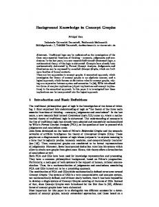
The Information Technology Institute Vietnam National University, Hanoi Hanoi, Vietnam [email protected] algorithms have been proposed in literature to deal with different problem domains and scenarios. These include methods such as partition-based, density-based, graph-based, distance-based, and probability-based [21]. Among them, the field of graph clustering has grown quite popular with a vast number of published proposals for clustering algorithms as well as reported applications recently introduced. Graphs are structures formed by a set of vertices (also called nodes) and a set of edges that are connections between pairs of vertices. The core idea of a graph clustering algorithm is that grouping the vertices of a given input graph into clusters, taking into consideration the edge structure of the graph in such a way that there should be many edges within each cluster and relatively fewer between the clusters. Our work was inspired by graph-based clustering. One can find information about them in survey on graph clustering by Schaeffer[15]. Additionally, in general, standard data clustering is closely related to unsupervised learning meaning that there is no outcome variable nor is anything known about the relationship between the observations in the data set. In many situations, background knowledge about the clusters is available in addition to the values of features. For example, the cluster labels of some observations may be known (called seeds), or certain observations may be known to belong (or not) to the same cluster (pairwise constraints). One may wish to incorporate this information to the clustering process in order to (1) boost the performance of clustering, (2) bias the search of the algorithm toward the solutions are more consistent with background knowledge, (3) improve the quality of the result reducing the algorithm natural bias, or (4) identify clusters that are associated with a particular outcome variable. As a result, in the past two decades, semi-supervised clustering has received a great deal of attention [5]. We can note here the semi-supervised K-means [4, 7], semi-supervised Fuzzy-C means [6], semi-supervised spectral clustering [13, 20], semi-supervised density based clustering [12], semi-supervised graph based clustering [10, 16], and graph clustering with constraints [2], to mention a few. Existing semi-supervised methods for clustering with background knowledge fall into two general approaches that are used either constraints or seeds. Constraints involve must-link and cannotlink constraints in which the must-link constraint between two observations x and y means that x and y should be in the same cluster, and the cannot link constraint means that x and y should not be in the same cluster. For seed side information, a small set of labeled instances (in contrary with supervised learning in which we need a big set of labeled instances to train a classifier model) will be provided for semi-supervised clustering algorithms. Figure 1 illustrates the spectrum of four types of prior knowledge that can be integrated in the process of classifying data [11]. In 2009, Kulis et al.[10] introduced their semi-supervised graph based clustering

SoICT ’17, December 7–8, 2017, Nha Trang City, Viet Nam

Viet-Vu Vu and Hong-Quan Do

Figure 1: Spectrum of supervised (a), partially labelled (b), constrained (c), and unsupervised (d) learning: dots correspond to points without any labels; points with labels are denoted by circles, asterisks and crosses. In (c), the must-link and cannot-link constraints are expressed by solid and dashed lines, respectively [11]. with pairwise constraints. They tried to unify vector-based and graph-based approaches. Given input data in the form of either vectors or graph and pairwise constraints, they applied kernel function to find clusters. By experiments, they demonstrated that for vectorbased data, the algorithm could discover clusters with non-linear boundaries in the input space and with the addition of constraints, the performance of graph clustering was be improved. In PAKDD 2011, Anand and Reddy [2] presented a graph based clustering with constraints. This algorithm based on CHAMELEON, a graph based hierarchical clustering algorithm. And recently, in 2017, the author Vu-Viet Vu [16] introduced a seed-based graph clustering, called SSGC. Using a graph of the k-nearest neighbors and a measure of local density for the similarity between vertex, SSGC integrates seeds in the process of building clusters and hence can improve the quality of clustering. It is worth noting that none of these works uses both kinds of background knowledge. Adopt the idea of constraint CHAMELEON and seed-based graph SSGC, we seek to extend SSGC method by effectively embedding both constraints and seed in the clustering process establishing a new semi-supervised graph-based clustering algorithm as we called MCSSGC. The Must-Link and Cannot-Link constraints are used as hints to bias the search of the algorithm toward solutions are more consistent with background knowledge. Experiments conducted on real data sets from UCI show that our method can boost the performance of clustering, producing good results compared with SSGC.

2 RELATED WORK 2.1 Preliminaries Given a data set X = {x 1 , x 1 , . . . , x n }, we review some concepts related to semi-supervised clustering algorithm as follows: Must-link: Must-link constraints specify that two instances have to be in the same cluster. Cannot-link: Cannot-link constraints specify that two instances cannot be in the same cluster. Seed: Let S ⊆ X , called the seed set, be the subset of data-points on which supervision is provided as follows: for each x i ∈ S, the user provides the cluster C L of the partition to which it belongs. We assume that corresponding to each partition C L of X , there is typically at least one seed-point x i ∈ S.

Semi-supervised clustering algorithm: In addition to the similarity information used by unsupervised clustering, in many cases a small amount of knowledge is available concerning either pairwise constraints (must-link or cannot-link) between data items or cluster labels (seeds) for some items. Instead of simply using this knowledge for the external validation of the results of clustering, one can wish to let it guide or adjust the clustering process, i.e. provide a limited form of supervision. In this case, the applied approach is called semi-supervised clustering. In fact, there are two kinds of semisupervised clustering which include constraint-based clustering and seed-based clustering. Generally, to develop a semi-supervised clustering algorithm, we have to find the way to integrate background knowledge in a given clustering algorithm.

2.2

Graph-based Clustering

Given a data set X = {x 1 , x 2 , . . . , x n }, the graph proposed in [8, 9] is expressed as a weighted undirected graph, in which each vertex represents a data point, and possesses at most k edges to its knearest neighbors. An edge is created between a pair of points, x i and x j , if and only if x i and x j have each other in their k-nearest neighbors set. The weight ω(x i , x j ) of the edge between two points x i and x j is defined as the number of common nearest neighbors the two points share, as shown in equation 1 as follow: ω(x i , x j ) =| N N (x i ) ∩ N N (x j ) |

(1)

where NN(.) denotes the set of k-nearest neighbors of the specified point. From the graph is defined as above, in [9], authors find clusters by partitioning the graph in clusters with a threshold θ . The limit of this algorithm is that it is difficult to find the θ . In [8], authors proposed an idea of combining density-based clustering and graphbased clustering to detect clusters of different sizes, shapes, and densities in noisy. Although the algorithm is a good idea, it still uses two parameters as DBSCAN.

2.3

Semi-supervised Graph-based Clustering by Seeding

In this section, we briefly review the semi-supervised graph based clustering (SSGC). SSGC uses set of seeds to overcome the limit of finding parameters in the partitioning step and needs only one

Graph-based Clustering with Background Knowledge


parameter that is the number of nearest neighbors of graph. SSGC includes two steps as follows [16]: Step 1: This step aims to partition a graph into some connected components by using a threshold θ in a loop: all edges which have weight less than θ will be removed to form connected components at each step. The value of θ is assigned to 0 at first step and is incremented by 1 after each step. This loop will stop when the following cut condition is satisfied: each connected component has at most one kind of seeds. After finding the connected components, main clusters will be built by propagating label in each connected component having at least one seed. Step 2: The purpose of this step is to detect noises and building final clusters. The remaining points (graph nodes) that do not belong to any main clusters will be divided into two sets: points that have edges which relate to one or more clusters and others points which can be considered as isolated. In the first case, points are assigned to the cluster with the largest related weight. For the isolated points in the second case, two choices are possible depending on the purposes of users: either remove them as noise or label them. The SSGC has shown the effectiveness compared with semisupervised density based clustering (SSDBSCAN).

2.4

In [2], Anand and Reddy presented a graph based clustering with constraints. This algorithm based on CHAMELEON, a graph based hierarchical clustering algorithm. The key idea of CHAMELEON is summarized as follows: Step 1: Construct a k-nearest neighbor graph Step 2: Partition the graph in to sub-clusters Step 3: Merge partitions to obtains final clusters The constrained CHAMELEON is simply using constraints (mustlink, cannot-link) for the step of constructing the k-NN graph (step 1). When we have a must-link constraint between u and v then the distance between u and v will be evaluated by: lim

distance(x i , x j ) − n = η

lim distance(x i , x j ) + n = λ

Adopt the idea of constraint CHAMELEON and seed-based graph SSGC, in this section, we propose a new semi-supervised graph based clustering with both constraints and seed integrated. We, therefore, named our algorithm MCSSGC. The proposed clustering algorithm is summarized in Algorithm 1 and could be explained as follows: Firstly, we use constraints in the construction of kNN-graph process. If exists a cannot-link constraint between x i and x j then we will not calculate the distance between x i and x j . In this step, the must-link constraints are used in the finding nearest neighbor set for each point of data. The step of partitioning graph in to sub-clusters is done similarity to SSGC algorithm. Finally, in the construction final clusters step, we use constraints to push subclusters or isolated points in clusters. The MCSSGC uses only one parameter that is the number of nearest neighbor. The θ is calculated automatically based on the cut condition.

Input: Data set X, number of neighbor k, a set of seeds S, a set of constraints C Output: A partition of X Process: 1: Embed constraints set C in the construction of k-NN graph 2: θ = 0 3: repeat 4: Connected component construction with threshold θ 5: θ =θ +1 6: until the cut condition is satisfied 7: Use constraints in propagation process of label to form principal clusters 8: Use constraints set C to construct final clusters

(2)

The meaning of equation 2 is that we bring any two points much closer to each other. In contrast, if we have a cannot-link constraint between u and v then the distance between u and v will be taken apart as far as possible (see equation 3). n→∞

GRAPH-BASED CLUSTERING WITH BACKGROUND KNOWLEDGE

Algorithm 1 MCSSGC Algorithm

Semi-supervised Graph-based Clustering with Constraints

n→dist ance(x i ,x j )

3

(3)

These parameters η and λ mentioned above are defined by: λ = Dmax × 10p

(4)

η = Dmin × 10−p

(5)

where Dmax and Dmin represents maximum and minimum distance values in the data matrix respectively. The constrained CHAMELEON has shown the effectiveness when compared to some other constrained clustering algorithms on some real data sets, however, there are so many parameters in the algorithm.

The algorithm complexity: As mentioned in [8], the complexity of the construction phase of k-NN graph is O(n 2 ) or O(nloдn) (if using an optimized structure of R-Tree with low dimension data). The complexity of the construction phase of the connected components is O(nk) where k is the number of neighbors in the kNN graph, using the method of breast first search (BFS) or depth-first search (DFS). So the complexity of our algorithm is O(n2 ) or O(nloдn) (if using R-Tree). It is the same as SSGC.

4 EXPERIMENT RESULTS 4.1 Datasets We use 6 well-known real data sets from the Machine Learning Repository [3], namely: Ecoli, Iris, Protein, Soybean, Thyroid, and Zoo to evaluate our algorithm. The details of the data sets are shown in Table 1. These data sets have been selected because they facilitate the reproducibility of the experiments and some of them have already been used in semi-supervised clustering articles.



Table 1: Details of the UCI data sets used for clustering

4.2

Data

#Objects

#Attributes

#Clusters

Ecoli

336

7

8

Iris

150

4

3

#Class

Protein

115

20

6

cp(cytoplasm)

143

Soybean

47

35

4

im(inner membrane without signal sequence)

77

Thyroid

215

5

3

pp(perisplasm)

52

Zoo

101

16

7

imU(inner membrane, uncleavable signal sequence)

35

om(outer membrane)

20

omL(outer membrane lipoprotein)

5

imL(inner membrane lipoprotein)

2

imS(inner membrane, cleavable signal sequence

2

Table 2: Ecoli Class Distribution

Evaluation Method

The data set used for the evaluation includes a correct answer or label for each data point. We use the labels in a post-processing step to evaluate the performance of our approach. The Rand Index (RI ) [14] is a measure of the similarity between two data clusterings. It is widely used in evaluation of clustering results. The RI measure computes the agreement between the theoretical partition of each data set and the output partition of evaluated algorithms. This n(n−1) measure is based on 2 pairwise comparisons between the n points of a data set X . For each pair of points x i and x j in X , a partition assigns them either to the same clusters or to different clusters. Let us consider two partitions P 1 and P2 , and let a be the number of decisions where the point x i is in the same cluster as x j in P1 and P2 . Let b be the number of decisions where the two points are placed in different clusters in both partitions. A total agreement can then be calculated as shown in equation 6. RI (P1 , P2 ) =

2(a + b) n(n − 1)

(6)

The value of RI is a number between 0 and 1 for the original version, in which, RI = 0 when the two clusterings have no similarities, while RI = 1 when the clustering are identical. In our experiments, we calculate RI in percentage. A higher the RI value indicates a the better performance of the clustering algorithm.

4.3

clustering accuracy even within a small number of seed in used, here is 11, compared to the accuracy of 96% with SSGC.

Comparative Results

To evaluate the effectiveness of our algorithm, we compare MCSSGC with the SSGC. Seeds for all the semi-supervised methods are randomly chosen in each time of running. Similarly, the must-link (ML) and cannot link (CL) constraints are also generated randomly from data. The results are averaged over 20 runs. The quality of clustering: Figure 2 (a-f) show the results obtained by the two algorithms. A glance at the graphs reveals in most cases a significantly better performance of MCSSGC compared to SSGC, indicating the benefit of using both seeds and constraints to build the clusters. We also note that MCSSGC uses only one parameter which is the number of nearest neighbor. Turning to the details, the improvement of MCSSGC is more pronounced for Soybean (Fig. 2-d) and Thyroid (Fig. 2-e) data set, that gives the two biggest improvement over SSGC, of around 4%. Especially for Soybean, the performance of MCSSGC reached 100%

#Objects

The another observation can be made is the result on Ecoli. Ecoli is a 7-dimensional data set consisting of 336 objects belonging to 8 classes. It is a highly unbalanced data set, having from 2 to 143 objects per class. The details of ecoli class distribution is shown in Table 2. Fig.2-a depicts the clustering result for Ecoli. In the first experiment with Ecoli data set, when using 30 seeds for both MCSSGC and SSGC, the performance of MCSSGC is lower than SSGC, even though for MCSSGC 140 constraints are in used. It is not surprising that there is a discussion regarding of the usefulness of a set of constraints, and how to find meaningful constraints for clustering process [12, 19]. The ML and CL constraints here play a role as hints to bias the clustering process, but most of these constraints has little practical value when they come from clusters with high separating reachability. Contribution of Must-Link and Cannot-Link Constraints in MCSSGC: To answer the question which Must-Link or CannotLink constraints are more beneficial in MCSSGC clustering process, we performed experiments as illustrated in Figure 3. A number of constraints for the method is randomly generated in each time of running, but one is with only must-link constraints and another is with a set of both must-link and cannot-link constraints. As explained, in the first step of MCSSGC, we use constraints in the construction of kNN-graph process. Here, if exists a cannot-link constraint between two data points, we will not calculate the distance between them. However, similarly to SSGC, MCSSGC uses seeds to partition a graph into connected components. Thus, cannot-link constraints make a little advantages in partitioning step. Must-link constraints, on the other hand, are used in the finding nearest neighbor set for each point of data. Experimental results in Figure 3 depict that MCSSGC with only Must-Link constraints outperforms in all experiments. Remarkably, the performance on Protein data set reached 92% clustering accuracy, an improvement of nearly 10% compared to MCSSGC (ML+CL). A fairly good result was also obtained with a difficult clustering data set like Ecoli, here the clustering accuracy is 93%. Furthermore, it can be seen that the more number of Must-Link constraints we have the more benefits we obtain. Such these results claim the key contribution of Must-Link constraints in our proposed algorithm.

Graph-based Clustering with Background Knowledge


Ecoli

Iris

95

95

90

90

Rand Index

100

Rand Index

100

85

80

85

80 MCSSGC

MCSSGC

75

75 SSGC

70 30/140

60/160

90/180

SSGC

70 35/100

120/200

Number of Seeds/Number of Pairwise Constraints

45/120

55/140

65/160


(a)

(b)

Soybean

Protein 90

100

85 95 80

Rand Index

Rand Index

90 75 70 65

85

80 60 MCSSGC

MCSSGC

75

55

SSGC

SSGC

50 18/80

20/100

22/120

70 11/60

25/140


12/70

13/80

14/90


(c)

(d)

Thyroid

Zoo

90

100 98

85 96 94

Rand Index

Rand Index

80

75

92 90 88

70 86 MCSSGC

65

SSGC

60 10/140

15/160

20/180


(e)

25/200

84

MCSSGC

82

SSGC

80 20/80

22/100

24/120

26/140


(f)

Figure 2: Comparison results between MCSSGC and SSGC on UCI data sets w.r.t Rand Index (the higher, the better).



Ecoli

Iris

100

100

95

95

90

90

Protein 100 95

85

80

Rand Index

Rand Index

Rand Index

90

85

80 75

80 MCSSGC (ML only)

75

70 30/140

85

MCSSGC (ML only)

75

MCSSGC (ML+CL)

60/160

90/180

120/200

70 35/100

MCSSGC (ML+CL)

45/120

55/140

70

MCSSGC (ML only)

65

MCSSGC (ML+CL)

60 18/80

65/160



(a)

20/100

(b)

Soybean 90

99

85

98

80

25/140

(c)

Thyroid

100

22/120


Zoo 100 99

97

Rand Index

Rand Index

Rand Index

98

75

96

96 95

70 MCSSGC (ML only)

95

94 11/60

97

65

MCSSGC (ML+CL)

12/70

13/80


14/90

60 10/140

15/160

MCSSGC (ML only)

94

MCSSGC (ML+CL)

93

20/180


(d)

(e)

25/200

92 20/80

MCSSGC (ML only) MCSSGC (ML+CL)

22/100

24/120

26/140


(f)

Figure 3: Comparison results between MCSSGC + Must-Link constraints only and MCSSGC + Must-link and Cannot-link constraints combined.

5

CONCLUSION

In this paper, a new graph based clustering algorithm with background knowledge is proposed. By using constraints in several phases of clustering process, MCSSGC algorithm obtains better results compared with SSGC. We also note that the problem of measuring constraints set is an interesting question. This means that how we can choose the good constraints for a given semisupervised clustering algorithm. There exists some works related to this topic such as active constraints selection [1, 18] or active seed selection [17], to mention a few. In future works, we will continue developing new semi-supervised clustering algorithms, active learning methods for selecting good background knowledge and applying for real applications in practice.

REFERENCES [1] A. A. Abin and H. Beigy. 2015. Active constrained fuzzy clustering: A multiple kernels learning approach. Pattern Recognition 48, 3 (2015), 953–967. [2] Rajul Anand and Chandan K. Reddy. 2011. Graph-Based Clustering with Constraints. In Proceeding of the Pacific-Asia Conference on Knowledge Discovery and Data Mining. 51–62. [3] A. Asuncion and D.J. Newman. 2015. UCI machine learning repository. (2015). http://www.ics.uci.edu/$\sim$mlearn/ [4] S. Basu, A. Banerjee, and R. J. Mooney. 2002. Semi-supervised Clustering by Seeding. In Proceeding of the Proceeding of 19th International Conference on Machine Learning. 281–304. [5] S. Basu, I. Davidson, and K. L Wagstaff. 2008. Constrained Clustering: Advances in Algorithms, Theory, and Applications. Chapman and Hall/CRC, 1 edition. [6] A. M. Bensaid, L. O. Hall, J. C. Bezdek, and L. P. Clarke. 1996. Partially Supervised clustering for image segmentation. Pattern Recognition 29, 5 (1996), 859–871.

[7] Mikhail Bilenko, Sugato Basu, and Raymond J. Mooney. 2004. Integrating constraints and metric learning in semi-supervised clustering. In Proceeding of the Proceeding of International Conference on Machine Learning. [8] L. Ertoez, M. Steinbach, and V. Kumar. 2003. Finding clusters of different sizes, shapes, and densities in Noisy, high dimensional data. In Proceeding of the SIAM International Conference on Data Mining. 47–58. [9] R. A. Jarvis and E. A. Patrick. 1973. Clustering using a similarity measure based on shared near neighbors. IEEE Transactions on Computer 22, 11 (1973), 1025–1034. [10] Brian Kulis, Sugato Basu, Inderjit S. Dhillon, and Raymond J. Mooney. 2009. Semi-supervised graph clustering: a kernel approach. Machine Learning 74, 1 (2009), 1–22. [11] Tilman Lange, Martin H. C. Law, Anil K. Jain, and Joachim M. Buhmann. 2005. Learning with Constrained and Unlabelled Data. In Proceeding of the CVPR. 731– 738. [12] L. Lelis and J. Sander. 2009. Semi-supervised Density-Based Clustering. In Proceeding of the IEEE International Conference on Data Mining. 842–847. [13] Dimitrios Mavroeidis. 2010. Accelerating spectral clustering with partial supervision. Data Min. Knowl. Discov. 21, 2 (2010), 241–258. [14] W.M. Rand. 1971. Objective criteria for the evaluation of clustering methods. American Statistical Association 66, 336 (1971), 846–850. [15] Satu Elisa Schaeffer. 2007. Graph clustering. Computer Science Review 1 (2007), 27–64. [16] Viet-Vu Vu. 2017. Semi-supervised graph based clustering. Intelligent Data Analysis (2017). Accepted. [17] Viet-Vu Vu and Nicolas Labroche. 2017. Active seed selection for constrained clustering. Intelligent Data Analysis 21, 3 (2017), 537–552. [18] Viet-Vu Vu, Nicolas Labroche, and B. Bouchon Meunier. 2012. Improving constrained clustering with active query selection. Pattern Recognition 45, 4 (2012), 1749–1758. [19] Kiri Wagstaff, Sugato Basu, and Ian Davidson. 2006. When Is Constrained Clustering Beneficial, and Why?. In Association for the Advancement of Artificial Intelligence(AAAI). [20] Xiang Wang, Buyue Qian, and Ian Davidson. 2014. On constrained spectral clustering and its applications. Data Min. Knowl. Discov. 28, 1 (2014), 1–30. [21] Rui Xu and Donald Wunsch II. 2005. Survey of clustering algorithms. IEEE Trans. Neural Networks 16, 3 (2005), 645–678.