Multicast Routing in Multi-Radio Multi-Channel Wireless Mesh Networks

IEEE TRANSACTIONS ON WIRELESS COMMUNICATIONS, VOL. 9, NO. 10, OCTOBER 2010

3031

Multicast Routing in Multi-Radio Multi-Channel Wireless Mesh Networks Tehuang Liu, Member, IEEE, and Wanjiun Liao, Fellow, IEEE Abstract—In this paper, we tackle the multicast problem with the consideration of the interference between multicast trees in multi-radio multi-channel wireless mesh networks (MR-MC WMNs). We consider a dynamic traffic model, i.e., multicast session requests arrive dynamically without any prior knowledge of future requests. Each node in the network acts as a Transit Access Point (TAP), and has one or multiple radios tuned to non-overlapping channels. We prove that in MRMC WMNs, the minimum cost multicast tree (MCMT) problem, i.e., finding the multicast tree with minimum transmission cost, is NP-hard. We then formulate the problem by an Integer Linear Programming (ILP) model to solve it optimally, and propose a polynomialtime near-optimal algorithm, called Wireless Closest Terminal Branching (WCTB), for the MCMT problem. To alleviate the interference between multicast trees (sessions), we present a polynomial-time algorithm that computes the minimum interference minimum cost path in MR-MC WMNs, and integrate it into WCTB without altering the performance bound of WCTB on the tree cost. The experimental study shows that the tree cost produced by WCTB is very close to the optimal and that the proposed algorithm for interference alleviation is effective. To the best of our knowledge, this is the first paper that studies the MCMT problem in MR-MC WMNs. Index Terms—Multi-radio multi-channel wireless mesh networks, multicast tree.

W

I. I NTRODUCTION

IRELESS mesh networks (WMNs) have received much attention in recent years due to its low up-front cost, easy network maintenance, robustness, and reliable service coverage [1], [2]. In such networks, packets are forwarded in a multi-hop fashion from the source node to the destination node. Each node in the network acts as a Transit Access Point (TAP), and is usually stationary and not power-constrained. Some nodes in the network may have direct connections to wired networks and serve as gateways for the other nodes to access the Internet. One crucial issue in WMNs is the capacity degradation problem [3]–[5] due to the interference between wireless links. Previous work [6], [7] shows that employing multiple nonoverlapping channels is an effective approach to overcoming this problem and many research efforts have been devoted to developing MAC protocols [8], [9], channel assignment

Manuscript received May 6, 2009; revised August 30, 2009; accepted July 8, 2010. The associate editor coordinating the review of this paper and approving it for publication was V. Bhargava. This work was supported in part by the Excellent Research Projects of National Taiwan University, under Grant Number 97R0062-06, and in part by the National Science Council (NSC), Taiwan, under Grant Number NSC982219-E-002-022. T. Liu was with the Department of Electrical Engineering, National Taiwan University, Taipei, Taiwan. He is now with MediaTek Inc., Taiwan. W. Liao (corresponding author) is with the Department of Electrical Engineering and the Graduate Institute of Communication Engineering, National Taiwan University, Taipei, Taiwan (e-mail: [email protected]). Digital Object Identifier 10.1109/TWC.2010.082310.090568

schemes [6], [10], and routing algorithms [7], [11] for multiradio multi-channel (MR-MC) WMNs. In this paper, with the goal of utilizing of radio resource efficient, we study the minimum cost multicast tree (MCMT) problem in MRMC WMNs, where the cost refers to the transmission cost required for a source to deliver one packet to a group of receivers. We consider a dynamic traffic pattern, i.e., multicast routing (session) requests arrive one by one without any prior knowledge of future requests. Every time a new multicast session arrives, the MCMT problem arises. In wired networks, the MCMT problem is known as the Steiner tree problem [12], which is defined as follows. Given a graph 𝐺 = (𝑉, 𝐸), a cost function on its edges, and a set of terminals 𝑋 ⊆ 𝑉 , the problem is to find a connected sub-graph of 𝐺 that spans all terminals in 𝑋 and has the minimum tree cost (i.e., the sum of the costs on all edges in this sub-graph is the minimum). This problem is proved to be NP-complete [12]. The Steiner tree problem has been well studied in the literature and several approximation algorithms have been proposed [13]–[17]. In particular, Robins and Zelikovsky [13] propose an algorithm for the Steiner tree problem with an approximation ratio of 1.55. Chlebik and Chlebikova [14] further prove that the Steiner tree problem cannot be approximated within 95/94 unless P=NP. Moving from wireline to wireless networks, the major concern of the MCMT problem becomes how to exploit the wireless broadcast advantage [18] to save radio resource. Specifically, when a wireless node forwards a multicast packet to one of its neighbors, all the other neighbors will also receive this packet due to the broadcast nature of wireless communications. Therefore, the total consumption of radio resource is determined by the number of nodes that forward the multicast packets (i.e., the number of invoked transmissions), rather than the costs of links of the multicast tree as in wired networks. The MCMT problem in WMNs is proved to be NPcomplete by Ruiz and Gomez-Skarmeta [19]. Some heuristics for constructing multicast trees in wireless multi-hop networks can be found in [19]–[22]. The MCMT problem in WMNs is exacerbated when nodes are allowed to use multiple channels for communications. This is because whether or not two nodes can communicate directly with one another is now determined not only by their locations but also by the set of channels they use [23]. A wireless node may not be able to communicate with all of its neighbors via a single radio (since they may listen on different channels). As a result, more than one transmission (issued on different channels) may be needed for a wireless node to forward a single multicast packet to some of its neighbors. In [24], the authors propose a heuristic to construct a multicast structure for the network, and channels are assigned to nodes in the

c 2010 IEEE 1536-1276/10$25.00 ⃝

3032


network with the consideration of interference based on this multicast structure. However, their approach is not suitable for dynamic multicast traffic but for one single multicast session with determined traffic pattern. While the MCMT problem in wired networks is well studied [12]–[17], this problem receives less attention in WMNs [19]– [22], especially in MR-MC WMNs [24]. In this paper, we tackle the MCMT problem in MR-MC WMNs with a dynamic traffic model. We separate the routing problem from the channel assignment problem, and assume that the channel assignment is given and static [10]. This is because the traffic demand is unpredictable, and thus solving the routing problem along with the channel assignment problem for future multicast sessions in advance may be meaningless [7], [23]. The interplay between routing and channel assignment in MRMC WMNs can be found in our previous work in [25]. We prove that the MCMT problem in MR-MC WMNs is NPhard, and present an Integer Linear Programming (ILP) model to optimally solve the MCMT problem. We also propose a centralized polynomial-time near-optimal algorithm, called Wireless Closest Terminal Branching (WCTB), for the MCMT problem, and analyze its theoretical performance bound and complexity. Furthermore, we also consider load balancing across channels in our multicast routing algorithm. As we have mentioned earlier, to describe a multicast tree, we have to specify the constitutive nodes and the channels that they use to communicate. Channels may thus be unequally loaded if some channels are used for more multicast trees than the others. Since the load of a channel is location-dependent in wireless environments and can be captured by the local co-channel interference [5], [7], [11], our algorithm aims at distributing load across channels by minimizing the co-channel interference between multicast trees. We propose a polynomial-time algorithm that finds the minimum interference minimum cost path in MR-MC WMNs, and integrate it into WCTB without altering the performance bound of WCTB on the tree cost. The experimental study shows that the tree cost produced by WCTB is very close to the optimal and that the proposed algorithm for interference alleviation is indeed effective. To the best of our knowledge, this is the first paper that studies the MCMT problem in MR-MC WMNs. Overall, the main contributions of this paper include: 1) The MCMT problem in MR-MC WMNs is formally defined and formulated. The interference among multiple trees is also explored. 2) An ILP model for the MCMT problem is presented. It serves as a benchmark for evaluating the quality of the solutions obtained by any approximation algorithm for this problem. 3) Our mechanism is a polynomial time algorithm with near optimal performance. It is efficient and easy to implement. 4) Our mechanism supports multiple trees and is an online routing mechanism which accepts dynamic tree establishment requests without prior information on the requests. 5) Our mechanism finds a good solution which ensures a performance guarantee of the tree cost while causing low interference to existing trees.

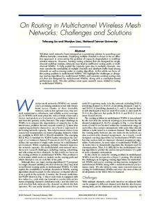
source A

A 1 1

D

1 3 5 5

3

4

Fig. 1.

2

4 2 5 U H 35 J 5 5

(a) The network graph.

2

B

L 3

2 1

2

B 1

1

2

1 D

1 3 5 5

L 3

2 4 2 5 U H 35 J 5 5 3

4

(b) An optimal multicast tree(shown in bold arrows) with a tree cost of 4

The MCMT problem in MR-MC WMNs.

The rest of this paper is organized as follows. In Section II, we describe the system model used in this paper. In Section III, we formally define the MCMT problem in MRMC WMNs, propose an ILP model for solving the MCMT problem optimally, and present WCTB. In Section IV, we extend WCTB to alleviate the interference between multicast trees. In Section V, we conduct simulations to evaluate the performance of the proposed algorithms. Finally, we conclude this paper in Section VI. II. N ETWORK M ODEL We consider a static MR-MC WMN. Each node in the network acts as a TAP [2], [3]. Some nodes in the network may be connected to the Internet directly and serve as gateways for the other nodes to access the Internet. Each node is equipped with one or multiple radios, each of which is tuned to a non-overlapping channel. The set of available channels in the system is denoted by 𝑄. We assume that the channel assignment is given and static. The network is represented by a directed multi-graph 𝐺 = (𝑉, 𝐸), where 𝑉 is the set of vertices, 𝐸 is the set of edges. 𝐺 is referred to as the network graph in this paper. Each vertex in 𝑉 corresponds to a wireless node in the network and each edge represents a link in the network. Each edge in 𝐸 is denoted by (𝑖, 𝑗)𝑘 , representing an link that is incident from node 𝑖 to node 𝑗 and operates on channel 𝑘. We assume that each radio has a common transmission range and a common interference range. A pair of directed edges (𝑖, 𝑗)𝑘 and (𝑗, 𝑖)𝑘 exist in 𝐸 between two vertices if the nodes 𝑖 and 𝑗 are located within the transmission range of each other and have a radio tuned to channel 𝑘. Figure 1(a) shows the network graph of a 7-node MR-MC WMN, where the number on each edge represents the channel on which this link operates. For example, nodes 𝐻 and 𝐽 can communicate with each other on channel 3 or 5, so there are four directed edges, (𝐻, 𝐽)3 , (𝐽, 𝐻)3 , (𝐻, 𝐽)5 , and (𝐽, 𝐻)5 in the network graph. III. C ONSTRUCTING M INIMUM C OST M ULTICAST T REES A. Problem Description We focus on on-line multicast routing in MR-MC WMNs. When a multicast routing request arrives in the system, the multicast tree problem arises in determining the paths for a source node to deliver its data to a group of receivers (terminals). The cost of a multicast tree is defined as the number of transmissions. The considered problem in this paper

LIU and LIAO: MULTICAST ROUTING IN MULTI-RADIO MULTI-CHANNEL WIRELESS MESH NETWORKS

is to find the minimum cost multicast tree (MCMT) in MRMC WMNs. For example, Fig. 1(b) depicts such an optimal multicast tree (in bold arrows) for the network graph shown in Fig. 1(a), where node 𝐴 is the source node (i.e., the doublecircled vertex) and nodes 𝐷, 𝐽, and 𝑈 are the terminals (grey vertices) of the new multicast session. There are four transmissions specified, namely, from node 𝐴 to node 𝐿 (on channel 2), from node 𝐿 to node 𝐽 (on channel 4), from node 𝐽 to both nodes 𝐻 and 𝑈 (on channel 5), and from node 𝐻 to node 𝐷 (on channel 5). Therefore, the total cost is four. In this paper, a multicast tree is represented by a set of directed edges. For example, the multicast tree shown in Fig. 1(b) is {(𝐴, 𝐿)2 , (𝐿, 𝐽)4 , (𝐽, 𝐻)5 , (𝐽, 𝑈 )5 , (𝐻, 𝐷)5 }. Note that there are five edges in the tree but the total transmission cost is only four. In this paper, a node is referred to as a transmitting node on channel k in multicast tree T if it is responsible for forwarding multicast data to its neighbor via channel 𝑘 in 𝑇 (i.e., 𝑇 contains a directed edge which is incident from this node and operates on channel 𝑘). For example, in the multicast tree shown in Fig. 1(b), node 𝐴 is a transmitting node on channel 2. In this paper, we use 𝑉 (𝑇, 𝑘) to denote the set of transmitting nodes on channel 𝑘 in multicast tree 𝑇 . We define the tree cost of a multicast tree as follows. Definition 1: Tree Cost: The tree cost of a multicast tree 𝑇 is defined as the sum of the numbers ∑of transmitting nodes on each channel in 𝑇 , i.e.,𝑐𝑜𝑠𝑡(𝑇 ) = 𝑘∈𝑄 ∣𝑉 (𝑇, 𝑘)∣. Definition 2: Minimum Cost Multicast Tree (MCMT) problem: An instance (𝐺, 𝑠, 𝑀 ) of the MCMT problem consists of a network graph 𝐺 = (𝑉, 𝐸), a source node 𝑠 ∈ 𝑉 , and a set of terminals 𝑀 ⊆ 𝑉 . The MCMT problem is to find such a multicast tree in 𝐺 that is rooted at 𝑠 and spans all terminals in 𝑀 with the least tree cost. In the rest of this paper, we refer to the MCMT problem in single-channel WMNs or in wired networks explicitly, but refer to the MCMT problem in MR-MC WMNs as the MCMT problem for short. The following theorem shows that the MCMT problem is NP-hard. Theorem 1: The MCMT problem is NP-hard. Proof: Since the special case of the MCMT problem, the MCMT problem in single-channel WMNs, is shown to be NP-complete in [19], it follows that the MCMT problem in MR-MC WMNs is NP-hard. B. An ILP Formulation We present an Integer Linear Programming (ILP) model to solve the MCMT problem optimally. This model can serve as a benchmark for evaluating the quality of solutions obtained by any approximation algorithm for the MCMT problem. Given an instance (𝐺, 𝑠, 𝑀 ) of the MCMT problem, the network topology and channel assignment are described by a set of binary variables {𝑐𝑖−𝑗,𝑘 : ∀𝑖, 𝑗 ∈ 𝑉, 𝑖 ∕= 𝑗, 𝑘 ∈ 𝑄}. 𝑐𝑖−𝑗,𝑘 equals one if a directed edge (𝑖, 𝑗)𝑘 exists in 𝐺, and zero otherwise. A solution, i.e., a multicast tree, is represented by a set of binary variables, {𝑋𝑖−𝑗,𝑘 : ∀𝑖, 𝑗 ∈ 𝑉, 𝑖 ∕= 𝑗, 𝑘 ∈ 𝑄}. 𝑋𝑖−𝑗,𝑘 equals one if the multicast tree includes a directed edge (𝑖, 𝑗)𝑘 , and zero otherwise. For example, the multicast tree shown in Fig. 1(b) specifies that only 𝑋𝐴−𝐿,2 , 𝑋𝐿−𝐽,4 , 𝑋𝐽−𝑈,5 , 𝑋𝐽−𝐻,5 , and 𝑋𝐻−𝐷,5 are set to one. Clearly, if a

3033

source A 1

2 1

2

B 1

FA-L=3 L

3

2 FL-J=3 4 2 5 U D H 35 J 5 5 5 FH-D=1 FJ-U=1 FJ-H=1 1 3 5

3

4

Fig. 2. An example to show the network flow model used in the ILP formulation.

directed edge (𝑖, 𝑗)𝑘 is included in the multicast tree, it must exist in 𝐺. Therefore, we have the following constraints. 𝑋𝑖−𝑗,𝑘 ≤ 𝐶𝑖−𝑗,𝑘 , ∀𝑖, 𝑗 ∈ 𝑉, 𝑖 ∕= 𝑗, ∀𝑘 ∈ 𝑄 We employ the network flow model used in [26] to ensure that the resulting multicast tree indeed spans all terminals in 𝑀 . The basic idea of this network flow model is described as follows. First, the source node 𝑠 injects ∣𝑀 ∣ units of energy into the multicast tree, where ∣𝑀 ∣ represents the number of terminals in 𝑀 . This energy flow is split at each branching vertex of the tree into sub-flows such that the amount of energy of each sub-flow for each sub-tree equals the number of terminals in that sub-tree. If a vertex that an energy flow goes through is a terminal, it consumes one unit of energy. Otherwise, it just relays the energy flow without consuming any energy. Using this flow model, we can guarantee that the resulting multicast tree indeed spans all of the terminals by ensuring that each terminal receives at least one unit of energy through the paths included in the tree. We let 𝐹𝑖−𝑗 denote the aggregate amount of energy going from vertex 𝑖 to vertex 𝑗 (on any channel). Consider the multicast tree shown in Fig. 1(b). The corresponding non-zero energy flows are shown in Fig. 2. First, the source vertex 𝐴 sends 3 units of energy to vertex 𝐿 (i.e., 𝐹𝐴−𝐿 = 3). Vertex 𝐿 relays this energy flow to vertex 𝐽 without consuming any energy (i.e., 𝐹𝐿−𝐽 = 3). Since vertex 𝐽 is a terminal, it consumes one unit of energy and then splits the remaining two units of energy equally for vertices 𝑈 and 𝐻, respectively (i.e., 𝐹𝐽−𝑈 = 1 and 𝐹𝐽−𝐻 = 1). Again, vertex 𝐻 just relays the energy flow to terminal 𝐷 without consuming any energy (i.e., 𝐹𝐻−𝐷 = 1). Finally, vertices 𝐷 and 𝑈 both receive 1 unit of energy. With the above network flow model, we have the following constraints. First, the∑ source node 𝑠 sends ∣𝑀 ∣ units of energy to the network, i.e., 𝑗∈𝑉,𝑗∕=𝑠 𝐹𝑠−𝑗 = ∣𝑀 ∣. ∑There are no input flows to the source node, i.e., 𝑗∈𝑉,𝑗∕=𝑠 𝐹𝑗−𝑠 = 0. Each terminal takes out one unit of energy from the passing energy flow while non-terminal vertices do not consume energy from the flow. Thus, we have the following constraints. ∑ ∑ 𝐹𝑗−𝑖 − 𝐹𝑖−𝑗 = 1, ∀𝑖 ∈ 𝑀. 𝑗∈𝑉,𝑗∕=𝑖

∑ 𝑗∈𝑉,𝑗∕=𝑖

𝐹𝑗−𝑖 −

𝑗∈𝑉,𝑗∕=𝑖

∑ 𝑗∈𝑉,𝑗∕=𝑖

𝐹𝑖−𝑗 = 0, ∀𝑖 ∈ 𝑉, 𝑖 ∈ / 𝑀, 𝑖 ∕= 𝑠.

3034


Finally, only when an edge between vertices 𝑖 and 𝑗 is included in the multicast tree is it possible that 𝐹𝑖−𝑗 > 0. The corresponding constraints are given as follows. ∑ ∣𝑀 ∣ ⋅ 𝑋𝑖−𝑗,𝑘 ≥ 𝐹𝑖−𝑗 , ∀𝑖, 𝑗 ∈ 𝑉, 𝑖 ∕= 𝑗. (1)

minimize subject to:

𝑘∈𝑄

X i − j ,k ≤ ci − j ,k ; ∀i, j ∈V , i ≠ j, ∀k ∈ Q

The constraints in (1) relate the 𝑋𝑖−𝑗,𝑘 variables to the flow variables 𝐹𝑖−𝑗 . Note that the optimization process excludes the case that two edges (operating on different channels) between the same two vertices are both included in the multicast tree. To obtain the objective function which minimizes the tree cost, we introduce a set of binary auxiliary variables, {𝑌𝑖,𝑘 : ∀𝑖 ∈ 𝑉, 𝑘 ∈ 𝑄} to our formulation. 𝑌𝑖,𝑘 equals one if node 𝑖 is a transmitting node on channel 𝑘 in the resulting multicast tree, and zero otherwise. This means that if there is a directed edge 𝑒 in the multicast tree that is incident from vertex 𝑖 and operates on channel 𝑘, then 𝑌𝑖,𝑘 = 1. Thus, we can write a set of constraints that relate the 𝑌𝑖,𝑘 variables to the 𝑋𝑖−𝑗,𝑘 variables as follows.

Σ Fs− j =| M |;

j∈V , j ≠s

Σ Fj−s = 0;

j∈V , j ≠ s

∀i ∈ M

Fi − j = 0; Σ Fj−i − j∈Σ V , j ≠i

∀i ∈V , i ∉ M , i ≠ s

j∈V , j ≠i

| M | ⋅Σ X i− j ,k ≥ Fi− j ; ∀i, j ∈V , i ≠ j

The number of transmitting nodes on channel 𝑘 in the multicast tree is the sum of 𝑌𝑖,𝑘 over all nodes in 𝑉 . According to Definition 1, the tree cost is the total number of transmitting nodes in the tree over all channels. Therefore, the objective function is: ∑∑ 𝑌𝑖,𝑘 . 𝑚𝑖𝑛𝑖𝑚𝑖𝑧𝑒

k∈Q

Yi,k ≥ X i− j ,k ; ∀i, j ∈V , i ≠ j, ∀k ∈ Q X i− j ,k ∈{0,1}; ∀i, j ∈V , i ≠ j∀k ∈ Q Fi − j ≥ 0; ∀i, j ∈V

𝑘∈𝑄 𝑖∈𝑉

C. An Approximation Algorithm for the MCMT problem Next, we propose a polynomial-time approximation algorithm, called Wireless Closest Terminal Branching (WCTB), for the MCMT problem. The main idea of WCTB is that at each step, one new branch is added to the current multicast tree to reach a new terminal (i.e., a receiver which has not been spanned by the current tree) that is closest to the source node. In WCTB, the cost of each link in the network graph is initialized to one. The crux is that when a new branch is included into the multicast tree, the costs of links may become zero (due to the broadcast advantage). Different from the algorithms for constructing multicast trees in wired networks [15], [27], WCTB intends to exploit the wireless broadcast advantage to reduce the tree cost. The beauty of WCTB is that it enjoys excellent performance (shown later), and is easy to implement based on Dijkstra’s algorithm. Before proceeding to elaborate on WCTB, we introduce the link classification in WCTB. We let 𝑇 denote the current tree constructed in WCTB. Note that the algorithm terminates when 𝑇 spans all terminals in 𝑀 . When a link, say (𝑖, 𝑗)𝑘 , is added to 𝑇 , the increased tree cost due to this new link depends on how the current tree grows. Normally, adding a new edge into 𝑇 increments the tree cost by one. However, if node 𝑖 is already a transmitting node on channel 𝑘 in 𝑇 before link (𝑖, 𝑗)𝑘 is added, the increased tree cost due to this link

Fi − j = 1; Σ Fj−i − j∈Σ V , j ≠i

j∈V , j ≠i

𝑌𝑖,𝑘 ≥ 𝑋𝑖−𝑗,𝑘 , ∀𝑖, 𝑗 ∈ 𝑉, 𝑖 ∕= 𝑗, ∀𝑘 ∈ 𝑄

For the optimal multicast tree shown in Fig. 1(b), we have 𝑌𝐴,2 = 1, 𝑌𝐿,4 = 1, 𝑌𝐽,5 = 1, and 𝑌𝐻,5 = 1, and thus the tree cost is 𝑌𝐴,2 + 𝑌𝐿,4 + 𝑌𝐽,5 + 𝑌𝐻,5 = 4. The ILP formulation for the MCMT problem is summarized in Fig. 3.

Σ Σ Yi,k

k∈Q i∈V

Yi,k ∈{0,1}; ∀i ∈V , ∀k ∈ Q Fig. 3.

The ILP formulation for the MCMT problem.

𝑇 is zero. This is because this new edge does not increase the number of transmitting nodes in 𝑇 , and thus does not increase the tree cost (see Definition 1). In this paper, we refer to such zero-cost directed links which are not included in the current tree as covered links. Note that in WCTB, links already included in 𝑇 also have zero cost since reusing these links to establish a new branch does not increase the tree cost. WCTB is formally presented in Algorithm 1 (Table I). The costs of links in the network graph are initialized to one, and 𝑇 is an empty set. Branches (paths) are then added one by one into 𝑇 until it spans all terminals in 𝑀 . At each step, a minimum cost path from the source node 𝑠 to a new terminal 𝑚 is selected to be integrated into 𝑇 , where the path cost is defined as the sum of the costs of its constituent links. This new path is a minimum cost path that has less cost than any other path from 𝑠 to any other new terminal (ties are broken arbitrarily). After a new path is added to 𝑇 , the costs of non-zero-cost links in the network are updated accordingly. Specifically, if the new path contains link (𝑖, 𝑗)𝑘 , each link (𝑖, 𝑥)𝑘 in the network becomes zero-cost, for any 𝑥 ∈ 𝑉 . The above procedure is repeated until all terminals in 𝑀 are spanned by 𝑇 . For example, Fig. 4 demonstrates the operations of WCTB. Fig. 4(a) shows the network graph, where node 𝐴 is the source node (shown as the double-circled vertex) and nodes 𝐷, 𝐿, and 𝑅 are the terminals (shown as grey vertices). The number on each link represents the channel the link operates on. At the beginning, the minimum costs from 𝐴 to nodes 𝐷, 𝐿, and


TABLE I A LGORITHM 1. W IRELESS C LOSEST T ERMINAL B RANCHING (WCTB)

Input: A network graph 𝐺 = (𝑉, 𝐸), a source node 𝑠 ∈ 𝑉 , and a set of terminals 𝑀 ⊆ 𝑉 . Output: A multicast tree 𝑇 . 1: for each 𝑒 ∈ 𝐸 do 2: 𝑐𝑜𝑠𝑡(𝑒) ← 1 /*initialize the link cost to one*/ 3: end for 4: 𝑇 ← {} /*initialize 𝑇 to an empty set*/ 5: while 𝑀 not empty do 6: run Dijkstra’s algorithm to compute the minimum cost from 𝑠 to each terminal 𝑚 ∈ 𝑀 , 𝑐𝑜𝑠𝑡(𝑠, 𝑚) /* where 𝑐𝑜𝑠𝑡(𝑥, 𝑦) denotes the minimum cost from node 𝑥 to node 𝑦 in 𝐺*/ 7: 𝑚 ← arg min𝑖∈𝑀 𝑐𝑜𝑠𝑡(𝑠, 𝑖) 8: 𝑝𝑎𝑡ℎ ← 𝑚𝑖𝑛 𝑐𝑜𝑠𝑡 𝑝𝑎𝑡ℎ(𝑠, 𝑚) /*𝑚𝑖𝑛 𝑐𝑜𝑠𝑡 𝑝𝑎𝑡ℎ(𝑥, 𝑦) returns a path with minimum cost from node 𝑥 to node 𝑦*/ 9: 𝑇 ← 𝑇 ∪ 𝑝𝑎𝑡ℎ 10: for each link (𝑖, 𝑗)𝑘 ∈ 𝑝𝑎𝑡ℎ do 11: for each link 𝑒 = (𝑖, 𝑥)𝑘 ∈ 𝐸 do 12: 𝑐𝑜𝑠𝑡(𝑒) ← 0 /*update the link cost*/ 13: end for 14: end for 15: 𝑀 ← 𝑀 − {𝑚} 16: end while 17: return 𝑇

source

1

source

1 B

A

1

1 1 3 3 1 H

1

B

1 D

1

1 1 3 3 1

2 21 1 2

J

H L

2

2 2

4 4

3 3 4 R

U

4

cost to terminal

1

D

L

R

1

2

3

(a) The network graph.

D

1 2 21 1 2

J

L

2

2 2

4 4

3 3 4

4

W

4

1

A

1

R

4

W

4

U

4

cost to terminal

L

R

1

2

(b) A path from node A to node D is added.

3035

current tree are updated accordingly, that is, the costs from 𝐴 to 𝐿 and 𝑅 become 1 and 2, respectively. Next, node 𝐿 is chosen as the new terminal to cover. Path {(𝐴, 𝐽)1 , (𝐽, 𝐿)2 } is integrated into the current tree. The resulting multicast tree is shown in Fig. 4(c). Again, the cost from node 𝐴 to node 𝑅, the only terminal not spanned by the current tree now, is updated to 1. To span node 𝑅, path {(𝐴, 𝐽)1 , (𝐽, 𝑊 )2 , (𝑊, 𝑅)4 } is combined with the current multicast tree, where the costs of links (𝐴, 𝐽)1 and (𝐽, 𝑊 )2 are both zero. The final multicast tree is shown in Fig. 4(d) with a tree cost of 3. Theorem 2: Given an instance of the MCMT problem, (𝐺 = (𝑉, 𝐸), 𝑠, 𝑀 ), WCTB runs in 𝑂(∣𝑉 ∣ ⋅ ∣𝐸∣ ⋅ ∣𝑀 ∣) time. Proof: Clearly, the complexity of Algorithm 1 is dominated by the 𝑤ℎ𝑖𝑙𝑒 loop in lines 5 to 16. Line 6 takes 𝑂(∣𝑉 ∣⋅log ∣𝑉 ∣+ ∣𝐸∣) time. Line 7 takes at most 𝑂(∣𝑀 ∣) time. Finding the shortest path in line 8 can be done in 𝑂(∣𝑉 ∣) time based on the results obtained in Line 6. The 𝑓 𝑜𝑟 loop in lines 10 to 14 takes at most 𝑂(∣𝑉 ∣ ⋅ ∣𝐸∣) time. Since the 𝑤ℎ𝑖𝑙𝑒 loop in lines 5 to 16 repeats at most ∣𝑀 ∣ times, the entire algorithm runs in 𝑂(∣𝑉 ∣ ⋅ ∣𝐸∣ ⋅ ∣𝑀 ∣) time. Definition 3: Radio Degree: Given a network graph 𝐺 = (𝑉, 𝐸), the radio degree of vertex 𝑣 ∈ 𝑉 on channel 𝑘, denoted by 𝑑𝑒𝑔𝑟𝑒𝑒(𝑣, 𝑘), is the number of edges in 𝐸 which are incident on vertex 𝑣 and operate on channel 𝑘. In this paper, we let 𝐷𝑚𝑎𝑥 denote the maximum radio degree in the network, i.e., 𝐷𝑚𝑎𝑥 =

max 𝑑𝑒𝑔𝑟𝑒𝑒(𝑣, 𝑘).

𝑣∈𝑉,𝑘∈𝑄

(2)

Theorem 3: The approximation ratio of WCTB is no more than (2 ⋅ 𝐷𝑚𝑎𝑥 ), i.e., 𝑐𝑜𝑠𝑡(𝑇𝑊 𝐶𝑇 𝐵 ) ≤ 2 ⋅ 𝐷𝑚𝑎𝑥 , 𝑐𝑜𝑠𝑡(𝑇𝑜𝑝𝑡 ) where 𝑐𝑜𝑠𝑡(𝑇𝑊 𝐶𝑇 𝐵 ) and 𝑐𝑜𝑠𝑡(𝑇𝑜𝑝𝑡 ) denote the tree costs produced by WCTB and the optimal tree, respectively. Proof: See the Appendix.

source

1 B

A

1

1 1 3 3 1 H

1

1 1

2 21 1 J

2 2

B

2 2

4

W

4

L

4 4

3 3 R

source

1

D

4 4

U

cost to terminal

1

(c) A path from node A to node L is added. Fig. 4.

1

1 1

4

D

2 21 1 J

2 2

2 2

W

4

L

4 4

3 3 R

R

1

1 1 3 3 1 H

A

4 4

U

tree cost = 3

(d) A path from node A to node R is added.

An example to demonstrate the operations of WCTB.

𝑅 are 1, 2, and 3, respectively. Therefore, the minimum cost path from 𝐴 to 𝐷 is selected, i.e., path {(𝐴, 𝐷)1 } is added to the tree, resulting in two covered links, namely (𝐴, 𝐵)1 and (𝐴, 𝐽)1 (shown in dashed arrows in Fig. 4(b)). The costs on the links from node 𝐴 to the terminals not spanned by the

IV. A LLEVIATING THE I NTERFERENCE B ETWEEN M ULTICAST T REES In the previous section, we focus on minimizing the cost of the multicast tree for a new multicast session. In addition to transmission cost, interference between links is another important issue to consider for routing in WMNs. Improper routing may cause severe interference, leading to packet losses, network congestion, and starvations. In this section, we study how to alleviate the interference between multicast sessions by carefully constructing multicast trees. Specifically, we aim at minimizing the interference between the new multicast tree (for the new multicast session) and the existing multicast trees while ensuring the resulting tree cost is bounded. Denote the set of nodes located within the interference range of node 𝑣 by 𝐼𝑁 (𝑣). A link (𝑥, 𝑦)𝑡 is said to be interfered by the transmission invoked by node 𝑣 on channel 𝑘 if 1) 𝑡 = 𝑘 and 2) 𝑦 ∈ 𝐼𝑁 (𝑣) or 𝑥 ∈ 𝐼𝑁 (𝑣). We use 𝐼𝐿(𝑣, 𝑘, 𝑇 ′ ) to denote the set of links in an existing multicast tree 𝑇 ′ that are interfered by node 𝑣 on channel 𝑘. For example, consider node 𝑃 in Fig. 5. We have 𝐼𝐿(𝑃, 2, 𝑇 ′ ) = {(𝐴, 𝐵)2 , (𝐿, 𝐴)2 } and

3036


interference range of node P multicast tree T′ source

B

W

3

U

2

A

2

1

P

L

2 3

H

J

2 I

Fig. 5. An example to illustrate the interference relationship between a multicast tree and a node, where links (𝐴, 𝐵)2 and (𝐿, 𝐴)2 are interfered by node 𝑃 on channel 2, and link (𝐻, 𝐽)3 is interfered by node 𝑃 on channel 3.

𝐼𝐿(𝑃, 3, 𝑇 ′ ) = {(𝐻, 𝐽)3 }. To quantify the interference between multicast trees, we define the Co-Channel Interference as follows. Definition 4: Co-Channel Interference: The node cochannel interference of a node 𝑣 on channel 𝑘 w.r.t. an arbitrary set of multicast trees 𝑇𝑠𝑒𝑡 is defined as ∑ 𝑁 𝐶𝐼(𝑣, 𝑘, 𝑇𝑠𝑒𝑡 ) = ∣𝐼𝐿(𝑣, 𝑘, 𝑇 ′ )∣. 𝑇 ′ ∈𝑇𝑠𝑒𝑡

The tree co-channel interference of a multicast tree 𝑇 ′ w.r.t. a set of multicast trees 𝑇𝑠𝑒𝑡 is defined as ∑ ∑ 𝑁 𝐶𝐼(𝑖, 𝑘, 𝑇𝑠𝑒𝑡 ). 𝑇 𝐶𝐼(𝑇 ′ , 𝑇𝑠𝑒𝑡 ) = 𝑘∈𝑄 𝑖∈𝑉 (𝑇 ′ ,𝑘)

The tree co-channel interference of a multicast tree 𝑇 ′ represents the total number of links in 𝑇𝑠𝑒𝑡 that are interfered by the transmitting nodes in 𝑇 ′ . Since paths are special cases of trees, Definition 4 is also applicable to paths. The cochannel interference of a path 𝑝 w.r.t. a set of multicast trees 𝑇𝑠𝑒𝑡 can be calculated as follows. ∑ ∑ 𝑁 𝐶𝐼(𝑖, 𝑘, 𝑇𝑠𝑒𝑡 ) 𝑇 𝐶𝐼(𝑝, 𝑇𝑠𝑒𝑡 ) = 𝑘∈𝑄 𝑖∈𝑉 (𝑝,𝑘)

=

∑

𝑁 𝐶𝐼(𝑖, 𝑘, 𝑇𝑠𝑒𝑡 ).

(3)

(𝑖,𝑗)𝑘 ∈𝑝

From (3), we know that if we assign each edge (𝑖, 𝑗)𝑘 in the network a weight 𝑁 𝐶𝐼(𝑖, 𝑘, 𝑇𝑠𝑒𝑡 ) and define the weight of a path as the sum of the weights of its constituent edges, the co-channel interference of a path is exactly the weight of this path. Definition 5: Minimum Interference Multicast Tree (MIMT) Problem: An instance (𝐺, 𝑠, 𝑀, 𝑇𝑠𝑒𝑡 ) of the MIMT problem consists of a network graph 𝐺 = (𝑉, 𝐸), a source node 𝑠 ∈ 𝑉 , a set of terminals 𝑀 ⊆ 𝑉 , and the set of existing multicast trees in the network 𝑇𝑠𝑒𝑡 . The MIMT problem is to find a multicast tree 𝑇𝑛𝑒𝑤 that is rooted at 𝑠 and spans all terminals in 𝑀 with the least tree co-channel interference w.r.t. 𝑇𝑠𝑒𝑡 . The MIMT problem can be easily proved to be NP-hard with the reduction from the MCMT problem in single-channel

WMNs [19]. Clearly, it is very difficult to solve the MCMT problem and the MIMT problem at the same time, i.e., to find a multicast tree that has the least tree cost and the least tree co-channel interference. To jointly tackle these two problems, we extend WCTB by replacing the min cost path procedure used in WCTB (see line 8 in Algorithm 1) with a polynomialtime algorithm, called Minimum Interference Minimum Cost Routing (MIMCR). Given a source node and a destination node, MIMCR computes the minimum interference minimum cost path, which is defined as a path that has the least path co-channel interference among all minimum cost paths. Since the returned path of MIMCR is still a minimum cost path, the performance bound of WCTB on the tree cost remains the same, i.e., Theorem 3 still holds for WCTB with this extension. Note that there are three reasons why we may not be able to find the path with the minimum cost and also the minimum path co-channel interference. First, since the path cost and the co-channel interference of a path are two additive metrics, finding an optimal path with two additive metrics is NP-complete [28]. Second, such an optimal path may not even exist in the network because minimizing the path cost and minimizing the interference of a path tend to be two conflicting objectives [7], [11], [23]. Third, it is shown in [29] that taking low-interference (but maybe more costly) paths may not be beneficial to the system performance in terms of throughput in the long run, so we give the transmission cost precedence over the co-channel interference. We describe MIMCR in details as follows. As in Section III-C, we let 𝑇 denote the current multicast tree in WCTB. The set of existing multicast trees in the network is denoted by 𝑇𝑠𝑒𝑡 . Suppose MIMCR is called in WCTB to compute a minimum interference minimum cost path from the source node 𝑠 to a new terminal 𝑚. First, MIMCR constructs an auxiliary directed acyclic graph 𝐺𝑎𝑢𝑥 = (𝑉, 𝐸 𝑎𝑢𝑥 ), a subgraph of 𝐺 = (𝑉, 𝐸), which excludes edges in 𝐸 that must not appear in any minimum cost path from 𝑠 to 𝑚. Note that the costs of links are maintained by WCTB, i.e., only links in 𝑇 and covered links have a link cost of zero. For each edge 𝑒 = (𝑖, 𝑗)𝑘 in 𝐺𝑎𝑢𝑥 , its link weight is set to 𝑁 𝐶𝐼(𝑖, 𝑘, 𝑇𝑠𝑒𝑡 ∪{𝑇 }) if it is not in 𝑇 or it is not a covered link. Otherwise, its link weight is set to zero, because including such an edge into the multicast tree does not result in any new transmitting node on any channel and thus does not increase the co-channel interference of the tree. The minimum interference minimum cost path from 𝑠 to 𝑚 is the path with the least weight in 𝐺𝑎𝑢𝑥 , which can be obtained by Dijkstra’s algorithm. The running time of MIMCR is dominated by the computation of the link co-channel interference for edges, which can be done in 𝑂(∣𝐸∣2 ⋅ ∣𝑇𝑠𝑒𝑡 ∣). Fig. 6 demonstrates the operations of MIMCR. Fig. 6(a) shows the network graph 𝐺 and the current multicast tree 𝑇 (bold arrows), where the number on each link represents the channel on which it operates. Link (𝐴, 𝐻)1 is a covered link, so its link cost is zero. Links (𝐴, 𝐵)1 and (𝐵, 𝐿)2 also have zero cost since they are included in 𝑇 . Suppose that a minimum interference minimum cost path from node 𝐴 (source node) to node 𝑃 (the new terminal) is required. There are only three minimum cost paths from 𝐴 to 𝑃 in 𝐺, that is, 𝑝1 = {(𝐴, 𝐻)1 , (𝐻, 𝑊 )1 , (𝑊, 𝑃 )4 },


Fig. 6.

H

B 0 7

L I

4

12 9

W 8

P

J

An example to demonstrate the operations of MIMCR.

𝑝2 = {(𝐴, 𝐻)1 , (𝐻, 𝐼)3 , (𝐼, 𝑃 )3 }, and 𝑝3 = {(𝐴, 𝐵)1 , (𝐵, 𝐿)2 , (𝐿, 𝐽)2 , (𝐽, 𝑃 )4 }, all of which have a path cost of 2. Fig. 6(b) shows 𝐺𝑎𝑢𝑥 , which preserves all possible minimum cost paths from 𝐴 to 𝑃 in 𝐺. In Fig. 6(b), the number on each link now represents its link weight (pre-calculated based on 𝑇𝑠𝑒𝑡 and 𝑇 ). Note that the weights of links (𝐴, 𝐵)1 , (𝐵, 𝐿)2 and (𝐴, 𝐻)1 in 𝐺𝑎𝑢𝑥 are all zero because their link costs in 𝐺 are zero. By running Dijkstra’s algorithm, 𝑝1 is returned to WCTB as the new branch because it has the least path co-channel interference, i.e., 0 + 4 + 8 = 12, among 𝑝1 , 𝑝2 , and 𝑝3 . V. P ERFORMANCE E VALUATION In this section, we evaluate the performance of the proposed algorithms via simulations. Each simulated scenario is described by four parameters, namely 𝑓 , 𝑛, 𝑡, and 𝑐, where 𝑓 is the total number of multicast sessions, 𝑛 is the number of nodes placed in the network, 𝑡 is the number of terminals, and 𝑐 is the total number of available channels in the system. Multicast sessions arrive in the system one by one without any prior knowledge of future arrivals. The source node and the 𝑡 terminals of each multicast session are randomly selected. Each node has three radios. To decouple the effect of the channel assignment algorithm, the three radios of each node are tuned to three randomly selected distinct channels. All nodes are randomly placed within a 1000m×1000m square, and the transmission range and the interference range of each radio are set to 300m and 600m, respectively. We only consider connected networks and ignore orphan radios (i.e., radios that are tuned to channels not used by any neighboring node) [5], [23]. In the first scenario, we let 𝑓 = 20, 𝑛 = 31, and 𝑐 = 7, but vary 𝑡 from 5 to 30. We compare the tree cost produced by WCTB with the optimal value obtained by solving the ILP model presented in Section III using the LINDO mixed integer linear programming solver [30]. Figure 7a depicts the average tree cost for the first scenario, where the curve labeled unicast represents the number of transmissions needed for the source node to deliver one packet to each receiver via unicast and the curve labeled shortest path tree represents the

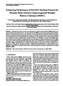
50 45 40 35 30 25 20 15 10 5 0

unicast shortest path tree WCTB optimal

25 20

15 10

5 5

10 15 20 25 number of receivers

0

30

a) Average tree cost of Scenario 1

11

(b) The auxiliary directed acyclic graph 𝐺𝑎𝑢𝑥 and the minimum interference minimum cost path (shown in shadowed arrows), where the number on each link is its weight in 𝐺𝑎𝑢𝑥 .

30 transmission cost

0

35


transmission cost

0

A

100 90 80 70 60 50 40 30 20 10 0


5

7

9

11

21

26 31 36 number of nodes

41

b) Average tree cost of Scenario 2 average tree co-channel interference

(a) The network graph and the current multicast tree (shown in bold arrows).

source

transmission cost

source A 1 1 1 B 2 1 1 1 2 H L 3 I 5 2 1 1 3 2 5 5 5 W 3 3 4 J 4 4 4 P

3037

220 200 180 160 140 120 100 80 60 40 20 0

WCTB WCTB with MIMCR

5 10 15 20 25 30 number of multicast sessions c) Average tree cost of Scenario 3 d) Average tree co-channel interference for Scenario 4

number of channels

Fig. 7.

Simulation results.

tree cost when the modified Pruned Dijkstra heuristic [15] is used. From this figure, we notice that the performance of WCTB is very close to the optimal and much better than the unicast delivery. In fact, from the simulation results, we find that the tree cost produced by WCTB is never more than twice of the optimal, even though 𝐷𝑚𝑎𝑥 in cases may be higher than 7. In the second scenario, we let 𝑓 = 20, 𝑡 = 15, and 𝑐 = 7, but vary 𝑛 from 21 to 41. Figure 7b shows the average tree cost for this scenario. As can be seen, the tree cost produced by WCTB is about 1.3 times of the optimal value, and only about one-third of the total transmission cost with unicast delivery. In the third scenario, we let 𝑓 = 20, 𝑛 = 31, and 𝑡 = 15, but vary 𝑐 from 5 to 11. The average tree cost is shown in Fig. 7c. Obviously, no matter how many channels are available in the network, WCTB always enjoys performance very close to the optimal. Moreover, from this figure, we notice that when more channels are available in the system, the tree cost may increase. This is because nodes tend to listen on different channels as more channels are used in the network, which in turn decreases the probability of enjoying the wireless broadcast advantage for multicasting. Note that an interference-aware channel assignment, which is typically intended to increase the channel diversity among nodes, may in general result in a high tree cost. In the last scenario, we let 𝑛 = 41, 𝑡 = 10, and 𝑐 = 7, but vary 𝑓 from 5 to 30. We compare the performance of pure WCTB and WCTB with MIMCR. Figure 7d shows the average tree co-channel interference. The simulation results show that MIMCR reduces the tree co-channel interference by about 48% on the average. For instance, when there are 30 multicast sessions (i.e., there are 30 multicast trees constructed), the average tree co-channel interference produced by pure WCTB is about 198 (i.e., on the average, the transmitting nodes in a multicast tree interfere with 198 links in the network) but

3038


with MIMCR it is down to 92. This proves that MIMCR is effective in alleviating the co-channel interference. VI. C ONCLUSION AND F UTURE W ORK In this paper, we tackle the MCMT problem with the consideration of interference between multicast trees in MRMC WMNs. We consider a dynamic traffic model. We prove that the MCMT problem is NP-hard and provide an ILP model for solving this problem optimally. A polynomial-time near optimal algorithm for the MCMT problem, WCTB, is then proposed. We further address the problem of minimizing the interference between multicast trees. A polynomial-time algorithm for computing the minimum interference minimum cost path between the source and the destination, MIMCR, is proposed. We extend WCTB by replacing the 𝑚𝑖𝑛 𝑐𝑜𝑠𝑡 𝑝𝑎𝑡ℎ() procedure in WCTB with MIMCR to alleviate the tree interference of the new multicast tree without altering the performance bound of WCTB on the tree cost. The simulation study shows that WCTB enjoys performance very close to the optimal, and that MIMCR can effectively reduce the interference between multicast trees. In the future, we will develop a multicast routing protocol which implements the WCTB and MIMCR algorithms. We also plan to extend WCTB to multi-rate environments, where nodes may communicate with each other at different data rates in order to combat channel deterioration. A PPENDIX P ROOF OF T HEOREM 3 Let 𝑇𝑜𝑝𝑡 denote the optimal multicast tree with tree cost 𝑐𝑜𝑠𝑡(𝑇𝑜𝑝𝑡 ), and 𝑇𝑊 𝐶𝑇 𝐵 denote the multicast tree computed by WCTB with tree cost 𝑐𝑜𝑠𝑡(𝑇𝑊 𝐶𝑇 𝐵 ). Given an instance (𝐺 = (𝑉, 𝐸), 𝑠, 𝑀 ) of the MCMT problem, we let 𝑡1 denote the source node, 𝑡𝑖+1 denote the 𝑖-th terminal in 𝑀 (ordered arbitrarily). Let 𝑑𝑖𝑠𝑡𝑎𝑛𝑐𝑒(𝑢, 𝑣) denote the shortest distance (in terms of hop count) from vertex 𝑢 to vertex 𝑣 in 𝐺. This proof needs the following two lemmas. Lemma 1: Suppose 𝑝1 , 𝑝2 , . . ., 𝑝𝑘 is a permutation of 1, 2, . . ., 𝑘. Then for every 𝑖, 2 ≤ 𝑖 ≤ 𝑘, there exists a unique critical pair (𝑝𝑗−1 , 𝑝𝑗 ) such that min(𝑝𝑗−1 , 𝑝𝑗 ) < 𝑖 ≤ max(𝑝𝑗−1 , 𝑝𝑗 ), 2 ≤ 𝑗 ≤ 𝑘. Proof: The proof can be found in [27]. Lemma 2: For any instance (𝐺 = (𝑉, 𝐸), 𝑠, 𝑀 ) of the MCMT problem, ∑∣𝑀∣ 𝑑𝑖𝑠𝑡𝑎𝑛𝑐𝑒(𝑡𝑝𝑖 , 𝑡𝑝𝑖+1 ) , 𝑐𝑜𝑠𝑡(𝑇𝑜𝑝𝑡 ) ≥ 𝑖=1 2 ⋅ 𝐷𝑚𝑎𝑥 where {𝑡𝑝1 , 𝑡𝑝2 , . . . , 𝑡𝑃∣𝑀 ∣ +1 } is a permutation of {𝑡1 , 𝑡2 , . . . , 𝑡∣𝑀∣+1 } obtained by a preorder traversal of 𝑇𝑜𝑝𝑡 starting from the source node 𝑠. Proof: For any two vertices 𝑢 and 𝑣 spanned by 𝑇𝑜𝑝𝑡 , let 𝑑𝑖𝑠𝑡𝑎𝑛𝑐𝑒(𝑢, 𝑣, 𝑇𝑜𝑝𝑡 ) denote the cost from vertex 𝑢 to vertex 𝑣 when the constituent edges of the available paths are restricted to the edge set, 𝐸𝑜𝑝𝑡 ≡ {(𝑖, 𝑗)𝑘 : (𝑖, 𝑗)𝑘 ∈ 𝑇𝑜𝑝𝑡 or (𝑖, 𝑗)𝑘 ∈ 𝑇𝑜𝑝𝑡 }. Clearly, 𝐸𝑜𝑝𝑡 ⊆ 𝐸, so we have 𝑑𝑖𝑠𝑡𝑎𝑛𝑐𝑒(𝑢, 𝑣, 𝑇𝑜𝑝𝑡) ≥ 𝑑𝑖𝑠𝑡𝑎𝑛𝑐𝑒(𝑢, 𝑣).

(4)

Let 𝑝𝑎𝑡ℎ𝑖 denote the path from 𝑡𝑝𝑖 to 𝑡𝑝𝑖 +1 when the constituent edges of the available paths are restricted to

𝐸𝑜𝑝𝑡 , where 1 ≤ 𝑖 ≤ ∣𝑀 ∣. The path length of 𝑝𝑎𝑡ℎ𝑖 is 𝑑𝑖𝑠𝑡𝑎𝑛𝑐𝑒(𝑡𝑝𝑖 , 𝑡𝑝𝑖 +1 , 𝑇𝑜𝑝𝑡 ). Consider a longer path 𝑝𝑎𝑡ℎ𝑐 that concatenates 𝑝𝑎𝑡ℎ1 , 𝑝𝑎𝑡ℎ2 , . . ., and 𝑝𝑎𝑡ℎ∣𝑀∣ sequentially. Since {𝑡𝑝1 , 𝑡𝑝2 ,...,𝑡𝑝∣𝑀 ∣ +1 } is a permutation of {𝑡1 , 𝑡2 , . . . , 𝑡∣𝑀∣+1 } obtained by a preorder traversal of 𝑇𝑜𝑝𝑡 starting from the source node 𝑠, the path length of 𝑝𝑎𝑡ℎ𝑐 is no more than the number of edges in 𝐸𝑜𝑝𝑡 , i.e., ∣𝑀∣ ∑

𝑑𝑖𝑠𝑡𝑎𝑛𝑐𝑒(𝑡𝑝𝑖 , 𝑡𝑝𝑖 +1 , 𝑇𝑜𝑝𝑡 ) ≤ ∣𝐸𝑜𝑝𝑡 ∣ ≤ 2 ⋅ ∣𝑇𝑜𝑝𝑡 ∣.

(5)

𝑖=1

In the following, we relate the size 𝑇𝑜𝑝𝑡 (i.e., ∣𝑇𝑜𝑝𝑡 ∣) to its cost (i.e., 𝑐𝑜𝑠𝑡(𝑇𝑜𝑝𝑡 )). According to Definition 3 and (2), in a tree, the number of edges that are incident from the same node and ∑ operate on the same channel is no more than 𝐷𝑚𝑎𝑥 . Thus, 𝑘∈𝑄 ∣𝑉 (𝑇𝑜𝑝𝑡 , 𝑘)∣ ⋅ 𝐷𝑚𝑎𝑥 ≥ ∣𝑇𝑜𝑝𝑡 ∣, where 𝑉 (𝑇𝑜𝑝𝑡 , 𝑘) denotes the set of transmitting nodes on channel 𝑘 in multicast tree 𝑇𝑜𝑝𝑡 . Therefore, according to Definition 1, we know 𝑐𝑜𝑠𝑡(𝑇𝑜𝑝𝑡 ) ⋅ 𝐷𝑚𝑎𝑥 ≥ ∣𝑇𝑜𝑝𝑡 ∣.

(6)

From (5) and (6), we obtain 2 ⋅ 𝑐𝑜𝑠𝑡(𝑇𝑜𝑝𝑡 ) ⋅ 𝐷𝑚𝑎𝑥 ≥ ∑∣𝑀∣ 𝑖=1 𝑑𝑖𝑠𝑡𝑎𝑛𝑐𝑒(𝑡𝑝𝑖 , 𝑡𝑝𝑖 +1 , 𝑇𝑜𝑝𝑡 ). Combining (4) with the equation above, we have ∑∣𝑀∣ 𝑖=1 𝑑𝑖𝑠𝑡𝑎𝑛𝑐𝑒(𝑡𝑝𝑖 , 𝑡𝑝𝑖 +1 , 𝑇𝑜𝑝𝑡 ) 𝑐𝑜𝑠𝑡(𝑇𝑜𝑝𝑡 ) ≥ 2 ⋅ 𝐷𝑚𝑎𝑥 ∑∣𝑀∣ 𝑑𝑖𝑠𝑡𝑎𝑛𝑐𝑒(𝑡 𝑝𝑖 , 𝑡𝑝𝑖 +1 ) 𝑖=1 ≥ . 2 ⋅ 𝐷𝑚𝑎𝑥 With the two lemmas above, we are now ready to prove Theorem 3. Recall that in WCTB, minimum cost paths are integrated into the current multicast tree 𝑇 one by one to span all terminals. Let 𝑚1 denote the source node and 𝑚𝑖+1 denote the 𝑖-th terminal spanned by the multicast tree in WCTB, where 1 ≤ 𝑖 ≤ ∣𝑀 ∣. Consider an arbitrary permutation of {𝑚1 , 𝑚2 , . . . , 𝑚∣𝑀∣+1 }, say {𝑚𝑝1 , 𝑚𝑝2 , . . . , 𝑚𝑝∣𝑀 ∣+1 }, where {𝑝1 , 𝑝2 , . . . , 𝑝∣𝑀∣+1 } is an arbitrary permutation of 1, 2, . . . , ∣𝑀 ∣ + 1. From Lemma 1, we know that for each 𝑖, 2 ≤ 𝑖 ≤ ∣𝑀 ∣+1, there exists a unique pair (𝑝𝑗−1 , 𝑝𝑗 ) such that min(𝑝𝑗−1 , 𝑝𝑗 ) < 𝑖 ≤ max(𝑝𝑗−1 , 𝑝𝑗 ), 2 ≤ 𝑗 ≤ ∣𝑀 ∣ + 1. In other words, for each terminal 𝑚𝑖 , 2 ≤ 𝑖 ≤ ∣𝑀 ∣+1, there exists a unique pair of terminals 𝑚𝑝𝑗−1 and 𝑚𝑝𝑗 such that one of 𝑚𝑝𝑗−1 and 𝑚𝑝𝑗 (denoted by 𝑛𝑖 ) must be included into the multicast tree earlier than 𝑚𝑖 and the other (denoted by 𝑛′𝑖 ) must be included into the tree no earlier than 𝑚𝑖 , i.e., 𝑛𝑖 = 𝑚min(𝑝𝑗−1 ,𝑝𝑗 ) and 𝑛′𝑖 = 𝑚max(𝑝𝑗−1 ,𝑝𝑗 ) . Thus, for 2 ≤ 𝑖 ≤ ∣𝑀 ∣ + 1, we have ∣𝑀∣+1

∑

∣𝑀∣+1

𝑑𝑖𝑠𝑡𝑎𝑛𝑐𝑒(𝑛𝑖 , 𝑛′𝑖 )

=

𝑖=2

∑

𝑑𝑖𝑠𝑡𝑎𝑛𝑐𝑒(𝑚𝑝𝑗−1 , 𝑚𝑝𝑗 ).

(7)

𝑗=2

In WCTB, to reach a new terminal, say 𝑚𝑖 , a minimum cost path from 𝑠 to 𝑚𝑖 is integrated. The cost of this minimum cost path is 𝑐𝑜𝑠𝑡(𝑠, 𝑚𝑖 ) = 𝑐𝑜𝑠𝑡(𝑚1 , 𝑚𝑖 ), so ∣𝑀∣+1

𝑐𝑜𝑠𝑡(𝑇𝑊 𝐶𝑇 𝐵 ) =

∑

𝑐𝑜𝑠𝑡(𝑚1 , 𝑚𝑖 ).

(8)

𝑖=2

In addition, since the link cost of edges in the current multicast tree 𝑇 in WCTB is zero, 𝑐𝑜𝑠𝑡(𝑚1 , 𝑚𝑖 ) is no more


than the distance (in terms of hop count) between 𝑚𝑖 and any terminal that is included in the current multicast tree, and thus and 𝑛𝑛𝑜−𝑒𝑎𝑟𝑙𝑖𝑒𝑟 , no more than the distance between 𝑛𝑒𝑎𝑟𝑙𝑖𝑒𝑟 𝑖 𝑖 i.e., for 2 ≤ 𝑖 ≤ ∣𝑀 ∣ + 1, 𝑐𝑜𝑠𝑡(𝑚1 , 𝑚𝑖 ) ≤ 𝑑𝑖𝑠𝑡𝑎𝑛𝑐𝑒(𝑛𝑒𝑎𝑟𝑙𝑖𝑒𝑟 , 𝑛𝑛𝑜−𝑒𝑎𝑟𝑙𝑖𝑒𝑟 ). 𝑖 𝑖

(9)

Combining (7), (8) and (9), we get ∣𝑀∣+1

𝑐𝑜𝑠𝑡(𝑇𝑊 𝐶𝑇 𝐵 ) ≤

∑

𝑑𝑖𝑠𝑡𝑎𝑛𝑐𝑒(𝑚𝑝𝑗−1 , 𝑚𝑝𝑗 ).

(10)

𝑗=2

The inequality in (10) holds if {𝑚𝑝1 , 𝑚𝑝2 , . . . , 𝑚𝑝∣𝑀 ∣+1 } is an arbitrary permutation of {𝑚1 , 𝑚2 , . . . , 𝑚∣𝑀∣+1 }. Therefore, it still holds if {𝑚𝑝1 , 𝑚𝑝2 , . . . , 𝑚𝑝∣𝑀 ∣+1 } is a permutation of {𝑡1 , 𝑡2 , . . . , 𝑡∣𝑀∣+1 } obtained by a preorder traversal of 𝑇𝑜𝑝𝑡 starting from the source node 𝑠, {𝑡𝑝1 , 𝑡𝑝2 , . . . , 𝑡𝑝∣𝑀 ∣+1 }. Accordingly, from Lemma 2 and (10), we have ∑∣𝑀∣ 𝑑𝑖𝑠𝑡𝑎𝑛𝑐𝑒(𝑡𝑝𝑖 , 𝑡𝑝𝑖 +1 ) 𝑐𝑜𝑠𝑡(𝑇𝑊 𝐶𝑇 𝐵 ) 𝑐𝑜𝑠𝑡(𝑇𝑜𝑝𝑡 ) ≥ 𝑖=1 ≥ . 2 ⋅ 𝐷𝑚𝑎𝑥 2 ⋅ 𝐷𝑚𝑎𝑥 Therefore, we obtain 𝑐𝑜𝑠𝑡(𝑇𝑊 𝐶𝑇 𝐵 ) ≤ 2 ⋅ 𝐷𝑚𝑎𝑥 . 𝑐𝑜𝑠𝑡(𝑇𝑜𝑝𝑡 ) R EFERENCES [1] I. F. Akyildiz, X. Wang, and W. Wang, “Wireless mesh networks: a survey,” Computer Networks J., pp. 445–487, 2005. [2] J.-F. Lee, W. Liao, and M.-C. Chen, “An incentive-based fairness mechanism for multi-hop wireless backhaul networks with selfish nodes,” IEEE Trans. Wireless Commun., no. 2, pp. 697–704, Feb. 2008. [3] T. Liu and W. Liao, “Location-dependent throughput and delay in wireless mesh networks,” IEEE Trans. Veh. Technol., no. 2, pp. 1188– 1198, Mar. 2008. [4] V. Gambiroza, B. Sadeghi, and E. W. Knightly, “End-to-end performance and fairness in multihop wireless backhaul networks,” ACM MOBICOM, 2004. [5] A. E. Gamal, J. Mammen, B. Prabhakar, and D. Shah, “Throughputdelay trade-off in wireless networks,” IEEE INFOCOM, 2004. [6] V. Gambiroza, B. Sadeghi, and E. W. Knightly, “End-to-end performance and fairness in multihop wireless backhaul networks,” ACM MOBICOM, 2004. [7] A. Raniwala and T.-C. Chiueh, “Architecture and algorithms for an IEEE 802.11-based multi-channel WMN,” IEEE INFOCOM, 2005. [8] T. Liu and W. Liao, “Interference-aware QoS routing for multi-rate multi-radio multi-channel WMNs,” IEEE Trans. Wireless Commun., no. 1, pp. 166–175, 2009. [9] J. Shi, T. Salonidis, and E. Knightly, “Starvation mitigation through multi-channel coordination in CSMA based wireless networks,” ACM MOBIHOC, 2006. [10] J. So and N. Vaidya, “Multi-channel MAC for ad hoc networks: handling multi-channel hidden terminals using a single transceiver,” ACM MOBICOM, 2004. [11] A. K. Das, H. M. K. Alazemi, R. Vijayakumar, and S. Roy, “Optimization models for fixed channel assignment in WMNs with multiple radios,” IEEE SECON, 2005. [12] R. Draves, J. Padhye, and B. Zill, “Routing in multi-radio, multi-hop WMNs,” ACM MOBICOM, 2004. [13] R.-M. Karp, “Reducibility among combinatorial problems,” Complexity of Computer Computations. New York: Plenum Press, 1975, pp. 85–103. [14] G. Robins and A. Zelikovski, “Improved Steiner tree approximation in graphs,” ACM-SIAM Symposium on Discrete Algorithms, 2000. [15] M. Chlebik and J. J. Chlebikova, “Approximation hardness of the Steiner tree problem on graphs,” Scandinavian Workshop on Algorithm Theory (SWAT), 2002.

3039

[16] S. Ramanathan, “Multicast tree generation in networks with asymmetric links,” IEEE Trans. Networking, pp. 558–568, 1996. [17] M. Charikar, C. Chekuri, and T.-Y. Cheung, “Approximation algorithms for directed Steiner problems,” J. Combinatorial Optimization, pp. 47– 65, 1997. [18] V. Melkonian, “New primal-dual algorithms for Steiner tree problems,” Computer and Operations Research, pp. 2147–2167, 2007. [19] J. E. Wieselthier, G. D. Nguyen, and A. Ephremides, “Energy-efficient broadcast and multicast trees in wireless networks,” Mobile Networks and Applications, pp. 481–492, 2002. [20] P. M. Ruiz and A. F. Gomez-Skarmeta, “Heuristic algorithms for minimum bandwidth consumption multicast routing in wireless mesh networks,” ADHOC-NOW, 2005. [21] H. Lim and C. Kim, “Multicast tree construction and flooding in wireless ad hoc networks,” ACM MSWiM, 2000. [22] A. Penttinen, “Efficient multicast tree algorithm for ad hoc networks,” MASS, 2004. [23] A. Penttinen, “Minimum cost multicast trees in ad hoc networks,” IEEE ICC, 2006. [24] T. Liu and W. Liao, “On routing in multi-channel wireless mesh networks: challenges and solutions,” IEEE Network, vol. 22, no. 1, pp. 13–18, Jan. 2008. [25] G. Zeng, B. Wang, Y. Ding, L. Xiao, and M. Mutka, “Multicast algorithms for multi-channel wireless mesh networks,” IEEE ICNP, 2007. [26] T. Liu and W. Liao, “Interplay of network topology and channel assignment in multi-radio multi-rate multi-channel wireless mesh networks,” IEEE GLOBECOM, 2008. [27] A. K. Das, R. J. Marks, M. El-Sharkawi, P. Arabshahi, and A. Gray, “Minimum power broadcast trees for wireless networks: integer programming formulations,” IEEE INFOCOM, 2003. [28] H. Takahashi and A. Matsuyama, “An approximate solution for the Steiner problem in graphs,” Math. Japonica, pp. 573–577, 1980. [29] Z. Wang and J. Crowcroft, “Quality-of-service routing for supporting multimedia applications,” IEEE J. Sel. Areas Commun., no. 7, pp. 1128– 1234, Sep. 1996. [30] Lindo milp solver. [Online]. Available: http://www.lindo.com Tehuang Liu received his BS and Ph.D. degrees in Electrical Engineering from National Taiwan University, Taiwan in 2004 and 2008, respectively. His research interests include performance analysis of multi-channel wireless mesh networks, routing protocols for multi-channel wireless mesh networks, and radio resource management in WiMAX networks. He is currently an engineer in MediaTek, Inc, Taiwan. Wanjiun Liao received her Ph.D. degree in Electrical Engineering from the University of Southern California, USA, in 1997. She is Professor of Electrical Engineering, National Taiwan University (NTU), Taipei, Taiwan, and an Adjunct Research Fellow of Research Center for Information Technology Innovation, Academia Sinica, Taiwan. Her research focuses on the design and analysis of wireless and multimedia networking protocols. Prof. Liao is currently an Associate Editor of IEEE T RANSAC TIONS ON W IRELESS C OMMUNICATIONS , and she has served on the editorial board of IEEE T RANSACTIONS ON M ULTIMEDIA. She has also served on the organizing committees of many international conferences, including serving as Tutorial Co-Chair of IEEE INFOCOM 2004, TPC Area Chair of IEEE International Conferences on Multimedia and Expo (ICME) 2004, TPC Vice Chair of IEEE GLOBECOM 2005 Symposium on Autonomous Networks, TPC Co-Chair of IEEE GLOBECOM 2007 General Symposium, TPC Co-Chair of IEEE VTC 2010 Spring and TPC Co-Chair of IEEE ICC 2010 Next Generation Networking and Internet Symposium. Prof. Liao has received many research awards and recognitions from different government and professional organizations, including IEEE and ACM. She was a recipient of the Republic of China (R.O.C.) Distinguished Women Medal in 2000. She is a Fellow of IEEE.