MULTICHANNEL NONNEGATIVE MATRIX FACTORIZATION IN ... - IRIT

MULTICHANNEL NONNEGATIVE MATRIX FACTORIZATION IN CONVOLUTIVE MIXTURES. WITH APPLICATION TO BLIND AUDIO SOURCE SEPARATION. Alexey Ozerov 1 and C´edric F´evotte 2 1

2 Institut TELECOM, TELECOM ParisTech, CNRS LTCI CNRS LTCI, TELECOM ParisTech 37-39, rue Dareau, 75014 Paris, France

{alexey.ozerov,cedric.fevotte}@telecom-paristech.fr

ABSTRACT We consider inference in a general data-driven object-based model of multichannel audio data, assumed generated as a possibly underdetermined convolutive mixture of source signals. Each source is given a model inspired from nonnegative matrix factorization (NMF) with the Itakura-Saito divergence, which underlies a statistical model of superimposed Gaussian components. We address estimation of the mixing and source parameters using two methods. The first one consists of maximizing the exact joint likelihood of the multichannel data using an expectation-maximization algorithm. The second method consists of maximizing the sum of individual likelihoods of all channels using a multiplicative update algorithm inspired from NMF methodology. Our decomposition algorithms were applied to stereo music and assessed in terms of blind source separation performance. Index Terms— Multichannel audio, nonnegative matrix factorization, nonnegative tensor factorization, underdetermined convolutive blind source separation. 1. INTRODUCTION Assume J signals (the sources) have been convolutively mixed through I noisy channels to produce I signals (the mixtures). Provided the filter lengths are “significantly” shorter than the analysis window size, the generative model may be formulated in the ShortTime Fourier Transform (STFT) domain such that xi,f n =

XJ j=1

aij,f sj,f n + bi,f n ,

(1)

where xi,f n is the complex-valued STFT of the i-th mixture (i = 1, . . . , I, f = 1, . . . , F is a frequency bin index, n = 1, . . . , N is a time frame index), sj,f n is the STFT of the j-th source (j = 1, . . . , J), aij,f is a frequency-dependent complex-valued mixing coefficient and bi,f n is residual noise. Eq. (1) can be rewritten in matrix form, such that xf n = Af sf n + bf n ,

(FD-ICA). The source labels remain however unknown because of the ICA standard permutation indeterminacy, leading to the wellknown FD-ICA permutation alignment problem. Many a posteriori alignment techniques relying on various source characteristics have been designed with various degrees of success, see e.g., [1] and references therein. The permutation ambiguity arises from the individual processing of each subband, which implicitly assumes mutual independence of one source’s subbands. This is not the case in this work where our frequency-dependent source model implies a coupling of the frequency bands, and joint estimation of the source parameters and mixing coefficients frees us from the permutation alignment problem. More precisely, our source model is inspired from NMF, and more specifically from NMF with the Itakura-Saito (IS) divergence which underlies a statistical model of superimposed latent Gaussian components, as described in [2] and summarized in Section 2. Section 3 addresses two inference methods in our proposed multichannel model. The first method, described in Section 3.1, consists of maximizing the exact joint log-likelihood of the multichannel data using an expectation-maximization (EM) algorithm [3]. This approach draws parallels with [4, 5], where source frames are assigned a Gaussian mixture model (GMM). However, our NMF model might be considered more suitable for musical signals than the GMM, and the computational complexity of exact inference in our model grows linearly with the number of components while the GMM’s complexity grows combinatorially. The second method, described in Section 3.2, consists of maximizing the sum of individual log-likelihoods of all channels using a multiplicative update (MU) algorithm inspired from NMF literature. This approach relates to recent nonnegative tensor factorization (NTF) techniques applied to multichannel music signals [6]. However, in contrast to standard NTF which implicitly assumes instantaneous mixing, our approach addresses a more general convolutive structure and does not require any post-processing binding step consisting of grouping the NTF elementary components into J sources. Section 4 reports BSS results of stereo music data and Section 5 provides conclusive remarks.

(2)

where xf n = [x1,f n , . . . , xI,f n ]T , sf n = [s1,f n , . . . , sJ,f n ]T , bf n = [b1,f n , . . . , bI,f n ]T and Af = [aij,f ]ij ∈ CI×J . Many convolutive blind source separation (BSS) methods have been designed under model (1). Typically, an instantaneous ICA algorithm is applied to data {xf n }n=1,...,N in each frequency subband f , yielding a set of J source subband estimates per frequency bin. This approach is usually referred to as frequency-domain ICA This work was supported in part by the French ANR project SARAH.

2. MODELS 2.1. Sources Let K ≥ J and {Kj }Jj=1 be a non-trivial partition of K = 1, . . . , K. We assume the complex random variable sj,f n to be a sum of #Kj latent components, such that sj,f n =

X k∈Kj

ck,f n

with

ck,f n ∼ Nc (0, wf k hkn )

(3)

where wf k , hkn ∈ R+ and Nc (µ, Σ) is a proper complex Gaussian distribution with probability density function (pdf) Nc (x|µ, Σ) = |π Σ|−1 exp −(x − µ)H Σ−1 (x − µ).

(4)

The components are assumed mutually independent and individually independent across frequency and frame. It follows that µ X ¶ sj,f n ∼ Nc 0, wf k hkn . (5) k∈Kj

Denoting Sj the F × N STFT matrix [sj,f n ]f n of source j and introducing the matrices Wj = [wf k ]f,k∈Kj and Hj = [hkn ]k∈Kj ,n respectively of dimensions F × #Kj and #Kj × N , it can easily be shown [2] that the log-likelihood of the parameters describing source j writes X − log p(Sj |Wj Hj ) = dIS (|sj,f n |2 |[Wj Hj ]f n ) + const. fn

where dIS (x|y) = x/y −log(x/y)−1 is the IS divergence. In other words, maximum likelihood (ML) estimation of Wj and Hj given source STFT Sj is equivalent to NMF of the power spectrogram |Sj |2 into Wj Hj , where the IS divergence is used. MU and EM algorithms are respectively described in [7, 8] and [2] for this task; in essence, this paper describes a generalization of these algorithms to a multichannel multisource scenario. Finally, we introduce the notation Pj = Wj Hj , i.e., pj,f n = E{|sj,f n |2 }.

previous assumptions, data xf n has a zero-mean proper Gaussian 2 distribution with covariance Σx,f n (θ) = Af Σs,f n AH f + σ b II , where Σs,f n = diag ([pj,f n ]j ) is the covariance of sf n . ML estimation is consequently shown to amount to minimization of 1 C1 (θ) =

³h

X fn

trace

i ´ −1 xf n xH f n Σx,f n + log det Σx,f n . (7)

The noise term σb2 II is here necessary to prevent from ill-conditioned inverses that may occur if one diagonal term of Σs,f n is close to zero, or if I > J. 3.1.2. Indeterminacies Criterion (7) suffers from scale, phase and permutation indeterminaˆ = {{Af }f , {Wj }j , {Hj }j } cies. Concerning scale and phase, let θ be a minimizer of (7) and let {Df }f and {Λj }j be a sets of respectively complex and nonnegative ¡ diagonal¢ matrices. Then, the set ˜ = {{Af D−1 }f , {diag [|djj,f |2 ]f Wj Λ−1 }j , {Λj Hj }j } θ j f ˆ = Σx,f n (θ), ˜ i.e., same likelihood value. Simleads to Σx,f n (θ) ilarly, permuted diagonal matrices would also leave the criterion unchanged. In Ppractice, we remove the scale and phase ambiguity by imposing i |aij,f |2 = 1 and a1j,fP∈ R+ (and scaling the rows of Wj accordingly) and by imposing f wf k = 1 (and scaling the rows of Hj accordingly).

2.2. Noise

3.1.3. Algorithm

In the most general case, we may assume noisy data and the following algorithms could accommodate estimation of noise statistics under Gaussian independent assumptions and given covariance structures such as Σb,f n = Σb,f or Σb,n . In this paper we assume for simplicity Σb,f n = σb2 II , where II is the identity matrix of size I and σb2 is a small and fixed noise variance. The noise component can account for both the quantization noise (if any) and possible model discrepancy in (1), and is required to prevent from potential numerical instabilities as discussed later.

We derive an EM algorithm [3] based on the complete data {X, C}, where C is the K × F × N STFT tensor with coefficients ck,f n . It can be shown that the family {p(X, C|θ)}θ is an exponential famP xf n s H ily [3] and the complete data statistics Rxs,f = f n /N , n P 2 Rss,f = n sf n sH f n /N and uk,f n = |ck,f n | form a natural (sufficient) statistics [3] for this family. Thus, one iteration of EM consists of computing the expectation of the natural statistics conditionally on the current parameter estimates (E step) and re-estimating the parameters using the updated natural statistics, which amounts to maximizing the conditional expectation of the complete data likeR lihood Q(θ|θ 0 ) = log p(X, C|θ)p(C|X, θ 0 )dC (M step). These steps are detailed in Algorithm 1.2 It can be easily checked that when the noise variance σb2 tends to zero, the resulting update rule for Af tends to Af ← Af . Similarly, the convergence of Af is very slow for small values of σb2 . To overcome this difficulty we use a simulated annealing strategy consisting of artificially and linearly decreasing the noise variance over the iterations, from an arbitrary large value to the small, correct value used in criterion (7).

2.3. Convolutive mixing model revisited The mixing model (2) can be recast as: ~ f cf n + bf n xf n = A

(6)

~ f is the “exwhere cf n = [c1,f n , . . . , cK,f n ]T ∈ CK×1 and A tended mixing matrix” of dimension I × K, with elements defined by ~aik,f = aij,f if and only if k ∈ Kj . Thus, for every frequency bin f our model is basically a linear mixing model with I channels and K elementary Gaussian sources ck,f n , with structured mixing coefficients (i.e., subsets of elementary sources arrive from ¡ same di-¢ rections). Subsequently, we will note Σc,f n = diag [wf k hkn ]k the covariance of ck,f n . 3. METHODS 3.1. Maximization of exact likelihood with EM 3.1.1. Criterion Let θ = {A, W, H} be the set of all parameters, where A is the I × J × F tensor with entries aij,f , W is the F × K matrix with entries wf k and H is the K × N matrix with entries hkn . Under the

1 For a fixed f , the BSS problem described by Eq. (2) and (7), and the following EM algorithm, is reminiscent of works by Cardoso, see, e.g., [9], where a grid of the representation domain is chosen, in each cell of which the source statistics are assumed constant. This is not required in our case where we instead solve F parallel linear instantaneous mixtures tied across frequency by the source model. In [9] the ML criterion can be nicely recast as a measure of fit between observed and parameterized covariances, where the measure of deviation writes D(Σ1 |Σ2 ) = −1 trace(Σ1 Σ−1 2 ) − log det Σ1 Σ2 − I and Σ1 and Σ2 are positive definite matrices of size I × I (note that the IS divergence is obtained in the special case I = 1). Unfortunately this formulation cannot be used in our case because Σ1 = xf n xH f n is singular. 2 Equation (14) only ensures Q(θ m+1 |θ m ) ≥ Q(θ m |θ m ) so that our algorithm is strictly speaking only a generalized EM (GEM) algorithm.

Algorithm 1 EM algorithm (one iteration) • E step. Conditional expectations of natural statistics: X b xs,f = 1 R xf nˆ sH (8) fn N n X b ss,f = 1 R ˆ sf nˆ sH (9) f n + Σs,f n − Gs,f n Af Σs,f n N n h i ~ u ˆk,f n = ˆ cf n ˆ cH (10) f n + (Σc,f n − Gc,f n Af Σc,f n ) k,k

where −1 Gs,f n = Σs,f n AH f Σx,f n ,

ˆ sf n = Gs,f n xf n , ˆ cf n = Gc,f n xf n ,

Gc,f n

(11)

−1 ~H = Σc,f n A f Σx,f n , (12)

~ f , Σc,f n , Σs,f n , and Σx,f n from Sec. 2.3 and 3.1.1. with A • M step. Update the parameters: b xs,f R b −1 Af = R ss,f , ˆk,f n 1 Xu wf k = , N n hkn

(13) hkn

1 Xu ˆk,f n = . F wf k

(14)

f

• Normalize A, W and H according to Section 3.1.2.

3.1.4. Reconstruction of the sources Wiener reconstructions of the source STFTs are retrieved from Eq. (11). Time-domain sources may then be obtained through inverse STFT using an adequate overlap-add procedure with dual synthesis window. By conservativity of Wiener reconstruction the spatial images of estimated sources and the estimated noise sum ˆf, ˆ altogether to the original mix in STFT domain, i.e., A sf n and ˆ f n = σb2 Σ−1 xf n satisfy Eq. (2). Thanks to linearity of the b x,f n inverse-STFT, the reconstruction is conservative in time domain as well. 3.2. Maximization of individual likelihoods with MU rules 3.2.1. Criterion We now consider a different approach consisting of maximizing the P sum of individual channel likelihoods i log p(Xi |θ), hence discarding mutual information between the channels. This is equivalent to setting the off-diagonal terms of xf n xH f n and Σx,f n to zero in criterion (7), leading to minimization of X C2 (θ) = dIS (|xi,f n |2 |ˆ vi,f n ), (15) if n

where vˆi,f n is the variance structure defined by X X vˆi,f n = wf k hkn qij,f j

k∈Kj

(+σb2 ),

(16)

with qij,f = |aij,f |2 . For a fixed channel i, vˆi,f n is basically the sum of the source variances modulated by the mixing weights. 3.2.2. Indeterminacies Criterion (15) suffers from same scale, phase and permutations ambiguities as criterion (7), with the exception that ambiguity on the

phase of aij,f is now total as this parameter only appears through it squared-modulus. In the following, the scales are fixed as in Section 3.1.2. 3.2.3. Algorithm We describe for the minimization of C2 (θ) an iterative MU algorithm inspired from NMF methodology. Continual descent of the minimized cost function under this algorithm was observed in practice. The algorithm simply consists of updating each scalar parameter θl by multiplying its value at previous iteration by the ratio of the negative and positive parts of the derivative of the criterion wrt this parameter, namely θl ← θl .[∇θl C2 (θ)]− /[∇θl C2 (θ)]+ , where ∇θl C2 (θ) = [∇θl C2 (θ)]+ − [∇θl C2 (θ)]− and the summands are both nonnegative [2]. This ensures nonnegativity of the parameter updates, provided initialization with a nonnegative value. The resulting parameter updates are described in Algorithm 2, where “.” indicates element-wise matrix operations, 1N ×1 is a N -vector of ˆ i ) the F × N ones, qij the F × 1 vector [qij,f ]f and Vi (resp. V 2 matrix [|xi,f n | ]f n (resp. [ˆ vi,f n ]f n ). Algorithm 2 MU rules (one iteration) h i ˆ .−2 .(Wj Hj ).Vi 1N ×1 V i i qij ← qij . h ˆ .−1 .(Wj Hj ) 1N ×1 V i PI ˆ .−2 .Vi )HTj diag(qij )(V i Wj ← Wj . i=1 PI ˆ .−1 HT diag(q ) V ij i j i=1 PI T ˆ .−2 (diag(qij )Wj ) (Vi .Vi ) Hj ← Hj . i=1 PI T ˆ .−1 i=1 (diag(qij )Wj ) Vi

(17)

(18) (19)

Normalize Q, W and H according to Section 3.2.2.

3.2.4. Reconstruction of the source images An image sim ij,f n of source j in channel i is reconstructed through sˆim vi,f n ) xi,f n , i.e., through Wiener filtering of ij,f n = (qij,f pi,f n /ˆ each channel. A noise component (if any) can similarly be reconstructed as ˆbi,f n = (σb2 /ˆ vi,f n ) xi,f n . Overall the decomposition is P ˆ conservative, i.e., j sˆim ij,f n + bi,f n = xi,f n . 4. RESULTS 4.1. Test material We produced J = 3 musical sources (drums, lead vocals and piano) using original separated tracks from the song “Sunrise” by S. Hurley (http://ccmixter.org/shannon-hurley). We selected 17 seconds-excerpts, that were converted to mono and downsampled to 16 kHz. The musical sources were mixed into a stereo recording using filters from the Source Separation Evaluation Campaign SiSEC 2008 development dataset 3 (http://sisec. wiki.irisa.fr/tiki-index.php). The test material, separation results and separation examples from original CD recordings are available at http://perso.telecom-paristech.fr/ ˜ozerov/demos.html#icassp09. 3 The reverberation time is 130 ms, distance between the two microphones is 1 m, distance between sources and the center of the microphone pair is about 1 m and the angles of arrival are -50, -10, and 15 degrees.

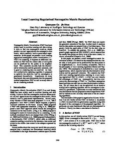
4.2. Simulations We have run 5000 iterations of both methods (EM and MU) from 10 random initializations of θ, with K = 12 components equally distributed between the 3 sources (i.e., #Kj = 4). Figure 1 plots the cost values C1 (θ) and C2 (θ) along iterations for the 10 runs. Note that because of the simulated annealing (Sec. 3.1.3) the EM’s cost C1 (θ) is not always decreasing (C1 (θ) is always computed with the small arbitrarily fixed noise variance σb2 , while the noise variance used in the EM algorithm changes with iterations). However, Figure 1 shows that the final value of C1 (θ) is always minimal. EM algorithm

7

10

C2(θ) cost value

C1(θ) cost value

MU rules

7

10

6

10

6

10

5

10 0 10

1

10

2

10

3

10

4

10

0

10

iteration number

1

10

2

10

3

10

4

10

iteration number

Fig. 1. 10 runs of EM and MU from random initializations. In our MATLAB implementation, 1000 iterations of EM (resp. MU) take about 80 min (resp. 20 min). Source images were reconstructed from the set of parameters obtained at the end of every run and source separation evaluation criteria were computed from the original and reconstructed images: the Signal to Distortion Ratio (SDR), the Image to Spatial distortion Ratio (ISR), the Source to Interference Ratio (SIR), and the Sources to Artifacts Ratio (SAR) [10]. For each method and every run, all evaluation criteria values were averaged over J = 3 sources. Table 1 displays for each method the evaluation criteria corresponding to (i) the best average SDR value obtained among the 10 runs, (ii) the best (i.e., minimal) cost value, along with reference values (in braces) computed from sources estimates as reconstructed from the corresponding randomly initialized parameters θ (0) . Algorithm Condition Av. SDR Av. ISR Av. SIR Av. SAR

EM algorithm best SDR best cost 4.3 (-1.0) 0.2 (-1.4) 8.1 (2.4) 3.8 (2.5) 6.5 (-3.1) 0.0 (-2.3) 10.0 (9.9) 9.2 (7.6)

MU rules best SDR best cost 3.6 (1.6) 0.4 (1.7) 8.0 (3.5) 4.6 (3.8) 6.9 (-2.7) 1.8 (-1.8) 7.3 (15.4) 7.6 (15.0)

Table 1. Source separation evalution criteria (dB).

5. DISCUSSION AND CONCLUSION Table 1 shows that both methods are very sensitive to initialization, and, unfortunately, the best value of the cost does not correspond to the best separation performance. However, the perceptual differences between the sources estimates are not always noticeable, and the numerical differences may be due to the nature of the criteria itself. Moreover, among only 10 random initializations at least one is leading to satisfying separation results. We are currently looking for better (non-random) initialization schemes.

Let us compare the two proposed methods. As compared to MU, the EM algorithm has the following advantages: (i) its convergence to a stationary point is theoretically proved, (ii) in contrast to the maximization of individual likelihoods, the maximization of the exact likelihood allows to better exploit the statistical dependencies between different channels, (iii) the EM algorithm allows for the estimation of the complex-valued mixing coefficients, while MU only estimate the absolute values of these coefficients 4 . As compared to EM, the MU algorithm has the following advantages: (i) convergence is faster (both in iterations and CPU time), (ii) the generalization of MU to other divergences used in NMF (e.g., Euclidean distance or Kullback-Leibler divergence) is straightforward. The new probabilistic framework presented in this paper addresses the representation of multichannel audio, under possibly underdetermined and noisy convolutive mixing. While we have assessed the validity of our model (with corresponding inference techniques) in terms of BSS, our model more generally provides a datadriven object-based representation of multichannel audio and could be relevant to other problems such as audio transcription and indexing. As such, it would be interesting to investigate the semantics revealed by the learnt dictionary W and corresponding activation patterns H; we leave this for future work. 6. REFERENCES [1] S. Makino, T.-W. Lee, and H. Sawada, Blind speech separation, Springer, 2007. [2] C. F´evotte, N. Bertin, and J.-L. Durrieu, “Nonnegative matrix factorization with the Itakura-Saito divergence. With application to music analysis,” Neural Computation, vol. 21, no. 3, Mar. 2009, Preprint at http://www.tsi.enst.fr/˜fevotte/ TechRep/techrep08_is-nmf.pdf. [3] A. P. Dempster, N. M. Laird, and D. B. Rubin., “Maximum likelihood from incomplete data via the EM algorithm,” Journal of the Royal Statistical Society. Series B (Methodological), vol. 39, pp. 1–38, 1977. [4] E. Moulines, J.-F. Cardoso, and E. Gassiat, “Maximum likelihood for blind separation and deconvolution of noisy signals using mixture models,” in Proc. IEEE International Conference on Acoustics, Speech, and Signal Processing (ICASSP’97), April 1997. [5] H. Attias, “New EM algorithms for source separation and deconvolution,” in Proc. IEEE International Conference on Acoustics, Speech, and Signal Processing (ICASSP’03), 2003. [6] D. FitzGerald, M. Cranitch, and E. Coyle, “Non-negative tensor factorisation for sound source separation,” in Proc. of the Irish Signals and Systems Conference, Dublin, Sep. 2005. [7] S. A. Abdallah and M. D. Plumbley, “Polyphonic transcription by nonnegative sparse coding of power spectra,” in Proc. 5th International Symposium Music Information Retrieval (ISMIR’04), Oct. 2004, pp. 318–325. [8] A. Cichocki, R. Zdunek, and S. Amari, “Csiszar’s divergences for non-negative matrix factorization: Family of new algorithms,” in Proc. 6th International Conference on Independent Component Analysis and Blind Signal Separation (ICA’06), Charleston SC, USA, 2006, pp. 32–39. [9] J.-F. Cardoso, H. Snoussi, J. Delabrouille, and G. Patanchon, “Blind separation of noisy Gaussian stationary sources. Application to cosmic microwave background imaging,” in Proc. 11e European Signal Processing Conference (EUSIPCO’02), 2002, pp. 561–564. [10] E. Vincent, H. Sawada, P. Bofill, S. Makino, and J. P. Rosca, “First stereo audio source separation evaluation campaign: Data, algorithms and results.,” in Proc. Int. Conf. on Independent Component Analysis and Blind Source Separation (ICA’07). 2007, pp. 552–559, Springer. 4 In the stereo case this translates to exploiting both the Interchannel Intensity Difference (IID) and the Interchannel Phase Difference (IPD) [10] in the case of EM, and by exploiting the IID only in the case of MU.