Multiclassifier Approach to Tagging of Polish - Semantic Scholar

Multiclassifier Approach to Tagging of Polish* Maciej Piasecki and Adam Wardyński Institute of Applied Informatics, Wrocław University of Technology Wybrzeże Wyspiańskiego 27, Wrocław, Poland [email protected]

Abstract. The large tagset, the limited size of corpora and the free word order are the main causes for achieving low accuracy of tagging Polish by applying the commonly used techniques based on stochastic modelling. The proposed architecture of the Polish tagger called TaKIPI created the possibility for using different types of classifiers in tagging, but only C4.5 Decision Trees were applied initially. The goal of this paper is to explore the range of promising rule based classifiers and to investigate their impact on the accuracy of tagging. Moreover, some simple techniques of combing the classifiers are also tested. The performed experiments showed that even a simple combination of different classifiers can increase the accuracy of the tagger by almost one percent.

1 Introduction The task of a tagger is to choose the appropriate morpho-syntactic description of a word among (possibly) many analyses assigned to it by a morphological analyzer. The problem of tagging is almost solved for many natural languages as taggers typically achieve for them the accuracy (calculated as the percentage of words properly described) higher than 95%. However it is not the case with tagging of Polish. The task is substantially more difficult and the size of the available training data is much smaller. In the largest corpus of Polish, namely IPI PAN Corpus (henceforth IPIC) [13], there are 4179 theoretically possible tags, but only 1642 of them occur in the manually disambiguated part of IPIC (henceforth MIPIC) i.e. 885 669 tokens. The low accuracy of Dębowski’s statistical tagger [2] constructed on the basis of MIPIC was caused mainly by the data sparseness. For English the number of tags is between 45 and 197 in different corpora [7], and but the size of a learning corpus is mostly greater than 1 million of tokens. However, a positional IPIC tag is a sequence of symbols describing different morphosyntactic features of a token (each feature is encoded in some tag attribute). Subsequences of some features occur in MIPIC more frequently than whole tags. Thus, the problem of the tagging of Polish can be decomposed into subproblems of partial disambiguation [12]. An architecture of a tagger facilitating this decomposition has been proposed and a Polish tagger, called TaKIPI [12], was constructed on this basis. *

Acknowledgement. This work was financed by the Ministry of Education and Science project No T11C 018 29

TaKIPI works on the basis of Decision Trees (C4.5 [14]) as the main classifiers combined with a limited set of handwritten rules. The change from stochastic modelling, as it was applied in [2], to symbolic rules was inspired by promising results obtained in [11] on tagging by rules acquired by the means of Genetic Algorithms (very inefficient unfortunately). However, TaKIPI achieved initially only 92.55% of accuracy. In the experiments presented in [10] the influence of handwritten rules and different types of constraints (operators) of different complexity as parts of Decission Trees were tested. These results showed that the more complex tagging rules achieve higher accuracy. As the room for improvements on the basis of C4.5 trees seems to be limited, we wanted to look for some other way of automatic extraction of tagging rules. The goal of this work is to analyse the possibility of application of other algorithms of rule extraction to the problem of tagging of Polish. As none of them appeared to be superior against the other ones, we performed some preliminary experiments on possibilities created by combining the classifiers. TaKIPI architecture, the role of rule-based classifiers and the general scheme of learning of classifiers are presented in Sec. 2. In Sec. 3, the results of application of the selected types of classifiers are given. And finally, in Sec. 4 we present the application of combined rule-based classifiers to the problem.

2 Architecture of the TaKIPI Tagger text Morfeusz

Reader & Pre-sentencer

Recogniser of Abbreviations

Filter of Rules

dictionary of abbreviations

hand-written rules unigram dictionary

Unigram Classifier layer masks Manager of Classifiers decision trees for layers

yes

Next layer?

DT 1

...

DD n

Annotator Sentencer & Writer tagged sentences

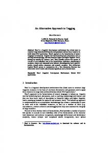
Fig. 1. The architecture of TaKIPI (Polish tagger).

The TaKIPI architecture is presented in Fig. 1. The process starts with morphosyntactic processing of the input text performed by Reader (based on morphological analyser Morfeusz [16]) and Abbreviation Recogniser. Each token is assigned a set of

possible tags i.e. its morpho-syntactic description. Next, the text is roughly divided into sentences (Pre-sentencer). The final decision concerning sentence boundaries is performed after tagging (Sentencer), because of ambiguity of some abbreviations. Filter of Rules applies a set of hand-written rules in order to delete some tags being impossible due to some general morpho-syntactic constraints. Initial probabilities for tags are calculated by Unigram Classifier on the basis of frequencies of: 〈token, tag〉, stored in the unigram dictionary. The probabilities for the pairs not observed in the learning data, but possible according to the morphological analysis, are calculated by smoothing based on Lidstone’s law (inspired by [8]). The core of the tagging process is divided into several subsequent phases. During each phase some tags can be deleted according to the performed partial disambiguation. The set of all possible tag attributes is divided into several layers. Attributes of the same layer are disambiguated during the same phase of tagging. During each phase, tags are distinguished only on the basis of values of attributes of the corresponding layer. A subset of tags of the given token such that all its members have identical values of attributes of the given layer is called a package of tags. During each phase, the tagger choose the best package according to the current probabilities of tags, and eliminates all packages except the best one. Each phase of tagging begins with subsequent applications of classifiers to each token in the sentence. More than one classifier can be applied to any token, as it often happens. Only tokens that are ambiguous with respect to the current layer are processed. The architecture is open for many types of classifiers. The only constraint is that a classifier should update the probabilities of tags. The way of calculating probabilities is unrestricted. In the present version of TaKIPI there are three layers: grammatical class, number and gender, and case. The other grammatical categories of IPIC are mostly dependent on the above (see [12]). In the first version of TaKIPI only classifiers based on the algorithm C4.5 of Induction of Decision Trees (DT) [14] were applied, but the architecture is open for any classifier under the condition that a classifier assigns probabilities to tags. The DT classifiers have been converted to classifiers returning the probabilities of: a positive decision — a selected value for some attribute, and a negative decision — a smoothed nonzero probability of other values, in a similar way to [8]. For each leaf of DT, the probability of its decision is calculated on the basis of the number of examples attached to this leaf during the tree construction. The probability is smoothed according to the algorithm presented in [8]. As in [8], instead of building one big classifier for a phase, we decided to decompose the problem further into the classes of ambiguity [8]. Each class corresponds to one of many possible combinations of values of layer attributes, e.g. there is only one attribute in the first layer, namely grammatical class, and different classes of ambiguity on the first layer are different combinations of grammatical classes observed in tokens of the learning data. Examples of classes of ambiguity are: {adj, subst}, {adj, conj, qub, subst} (where qub = particle-adverb ), or {sg, m1, m2, m3} (of the second layer: number singular, but all male genders possible). The number of examples for different classes of ambiguity varies to a large extent. For some classes there are thousands of examples, for some only few. Following [8], we

apply a kind of a backing off technique, in which an inheritance relation between ambiguity classes is defined. The inheritance relation is simply a set inclusion relation between sets of values defining ambiguity classes, e.g. `superclass' {adj fin subst} (where fin = verb non-past form) is in inheritance relation with {adj fin}, {adj subst}, etc. The construction of DT for a particular ambiguity class supports accurate choice of components of learning vectors for DT. We deliver to the given DT information specific for the given linguistic problem, e.g. concerning the distinction between nominative and genitive case. Thus, TaKIPI works on the basis of a collection of DTs divided into groups assigned to layers. Manager of Classifiers selects the proper set of DTs for each token which is ambiguous according to the current layer. Each DT multiplies the probabilities of tags in a token with the probabilities of a decision. Next, after processing of all tokens, only the package with the best maximal probability is left by Package Cut-off. At the end of the loop, probabilities in each token (only the winning package) are normalised. The process is repeated for each layer. On the basis of the analysis of a part of MIPIC, we identified all possible ambiguity classes for all layers. We selected some ambiguity classes, called supported classes that are sufficiently supported by examples (a heuristic criterion of having size about 100 examples) or are necessary according to the inheritance structure, i.e. the lack of linguistically reasonable superclass. Sets of learning examples are generated only for supported classes, but according to the inheritance hierarchy each token belonging to one of the non-supported classes is the source of learning examples added to the sets for its superclasses. A learning example is a sequence of values produced by a sequence of operators, where an operator can read a value of an attribute of some token or can express some compound logical constraints (e.g. testing some morpho-syntactic agreement) [10]. Generation of learning examples for the first layer is done in one iteration simultaneously for all ambiguity classes of this layer by sequentially setting the centre of the context in subsequent ambiguous tokens and applying operators of the appropriate ambiguity classes. For the next layers the process is identical, except the initial preparation of the learning data. During tagging, DTs (or generally classifiers) of the second layer are applied to tokens partially disambiguated. During learning, we have to create a similar situation. This is achieved by learning partial taggers for subsequences of layers up till the `full tagger'. Before preparation of learning examples for the k layer, a partial tagger for k-1 layers is applied and the attributes of all k-1 layers are disambiguated. This gradual learning appeared to be superior in comparison to an `ideal' disambiguation based on manual disambiguation of MIPIC. Summing up, TaKIPI utilises 131 classifiers dived into three layers and applied in the three subsequent phases. Thus the classifiers of one of the layers depend during training (description of learning examples) and tagging (combinations of values of attributes) on the classifiers of the previous layer in the sequence. It complicates the analysis of influence of a particular classifier on the final accuracy. The classifiers are rule based ones but they must produce probabilities of decisions. They do this on the basis of statistics collected during learning.

3 Selected single classifiers The first implementation of the TaKIPI architecture incorporated only classifiers based on C4.5 DT, but as the architecture is open to other types of classifiers, we aimed to select some classifiers that could possibly give better accuracy of tagging when used instead of C4.5. A version of TaKIPI utilising only classifiers of one type is called further a single classifier tagger. The learning sets produced by different ambiguity classes differ in size, balance and noise. Because of this, the selection of one type of classifier for the whole tagger cannot be based on any specific feature of the learning sets. The classifier actually should learn well on different types of learning sets. Moreover, we limited ourselves to rule based classifiers according to the reasons expressed in Sec. 1. Additionally, we focused on these types of classifiers that are reported to be competitive with C4.5 in literature. We took also into account the technical constraint of a classifier to be able to process the largest learning sets used in TaKIPI during training. Finally, the two rule based classifiers were selected: RIPPER [1] and PART [3]. The C4.5rules algorithm has been intentionally omitted, as we wanted to go further from C4.5 idea. However, as we need to get from a classifier a probability of decision, we were also interested in classifiers (non-binary) combining directly the extraction of rules with the estimation of probabilities. Logistic Model Trees classifier (LMT) [6] fulfils these criteria. It is a decision tree with logistic models in leaves, and logistic models directly define probability estimates. RIPPER and PART had to be altered to return probabilistic estimates, too. It has been done by simply getting the number of positive (or negative) examples covered by a rule and dividing this number by the total number of examples in the learning set. However, in addition to that, the assumption has been made that there always exist two bogus examples: one covered by all of the rules and the other one not covered by any of the rules. This is an idea somewhat similar to the smoothing used earlier for C4.5 trees1. We have to avoid returning zero probability. We cannot be sure that some decision is impossible and giving zero probability zeroes other decisions, for example made by the unigram classifier (the probabilities are multiplied). The training of the selected single classifiers were based on the slightly modified implementations of PART, RIPPER and LMT from the WEKA system [15]. The output files from WEKA were read and used in classification. We constructed our own implementations of the classifiers for the needs of the incorporation of them into the TaKIPI architecture (written in C++). All versions of single classifier taggers have been tested using 10-fold cross validation on the MIPIC. Also the C4.5 based original architecture was tested in order to establish a reliable baseline in relation to the modified implementation and the applied parameters of learning and tagging. The results are shown in Tab. 1. The tagging accuracy is presented in relation to all tokens (all) and to only ambiguous ones (amb). Besides the average results calculated 1

In fact the idea of smoothing as used in C4.5 has been tested on PART and proved to give slightly lower accuracy of tagging than the method described here. Therefore the type of smoothing used in C4.5 was not used with PART, nor with RIPPER.

on 10 folds (avg), the minimum and maximum (min and max) across the folds is presented too, in order to give an impression of the variance of the results. Table 1. Results of testing of single classifiers

Classifier C4.5 LMT RIPPER PART

avg 98.72 98.78 98.73 98.74

Classifier C4.5 LMT(& C4.5) RIPPER PART

avg 96.09 95.02 95.82 96.11

Classifier C4.5 LMT (& C4.5) RIPPER PART

avg 93.11 92.05 92.45 93.08

Layer 1 (≈ POS) all amb min max min avg 98.65 98.76 90.66 91.12 98.71 98.84 91.01 91.54 98.63 98.79 90.48 91.17 98.63 98.78 90.51 91.23 Layer 2 (L1 + number. gender) all amb min max min avg 95.88 96.26 87.33 87.92 94.70 95.24 83.71 84.62 95.61 95.96 86.50 87.08 96.00 96.24 87.70 88.01 Layer 3 (L2 + case) all amb min max min avg 92.94 93.40 85.40 85.71 91.79 92.29 83.02 83.52 92.11 92.79 83.68 84.34 92.87 93.34 85.26 85.64

max 91.39 91.84 91.46 91.46

max 88.36 85.17 87.55 88.30

max 86.23 83.92 85.02 86.16

The tagging errors made on the first layer, roughly corresponding to part of speeches, are the most important for practical applications. For the first layer, the best single classifier tagger appeared to be the LMT-based one. The statistical significance of the improvement is higher than 99.9% according to the T-test applied to the mean difference computed for the results of the 10 folds (e.g. [4]). The significances of all other results in this paper are calculated in the same way. Unfortunately LMT was extremely slow in training (weeks of computer work). For some of the largest learning sets completing of training was impossible due to technical limitations — the memory needed for Java Virtual Machine cannot exceed 1.5 GB and it appeared to be insufficient. In the second layer there were many classes of ambiguity for which we were unsuccessful with training LMT, instead C4.5 was used for these classes in LMT-based tagger. As the result, for the third layer we did not apply LMT at all. It means that in Tab. 1 the results described as LMT are the results achieved by a tagger in which LMT classifiers were applied to some classes of ambiguity, for the other ones C4.5 classifiers were used. Anyway, some preliminary experiments have shown that LMT classifiers for the third layer perform very poorly. Moreover, for the second layer the LMT performance (supplemented by C4.5) decreases and is exceeded by other classifiers (>99.9% of significance in comparison to C4.5 alone). An test case can have some attributes with values not seen and, therefore, not predicted on the basis of learning. LMT seems to be more sensitive to this problem than the other classifiers. LMT is partially DT but with logistic models in leaves,

and if an attribute with some unseen value occurs in a leaf, an inaccurate estimate of probability is generated by the model2. This is probably the reason why LMT accuracy is lower for the second and third layer. After the partial disambiguation according to the first layer some accidental combinations of attributes can appear. However, LMT is still the best classifier for the first layer for which the conditions are stable between learning and testing. The other classifiers are better suited for the situation in which some unseen values in data are encountered. Rules focus on values of attributes seen in learning data and at worst the last most generic rule is applied, the one that covers all examples that are not covered by the previous rules (both RIPPER and PART produce ordered sets of rules, where rules are applied one by one in a sequence). However there is still a notion, that when the previous layer gets disambiguated better, i.e. less tags are left for a token in some learning set, then it is harder to train the classifiers of the next layer on the basis of these sets. PART seems to cope best with this problem and it seems to be the best classifier from the tested ones, as it outruns C4.5 both on the first and the second layer and is only slightly worse on third layer. However, the significance of the PART results is low, about 90% in comparison to C4.5. Moreover, still, C4.5 surprisingly gets the best result for all three layers, but on the same level with PART for the third layer — the better result of C4.5 is statistically insignificant. The overall good result of C4.5 is obtained in contrast to the fact that it is not superior for the first layer, the most important one from the practical point of view. RIPPER seems to have also the better accuracy for the first layer in comparison to the baseline of C4.5, but without the statistical significance. PART is slightly better when used alone. The authors of PART say straight that their approach can be better than RIPPER, because PART avoids something they call hasty generalization, which is actually overpruning of the RIPPER’s rules. These results suggest that for some ambiguity classes (or even some cases) both classifiers can perform better than C4.5. We have to keep in mind that no optimization of learning parameters has been done. Adjusting of the parameters can lead to improvements, so maybe a tuned classifier other than C4.5 would be better for all layers, when used as a single classifier. The tuning of parameters was not the goal of this work, but in order to test this idea some general tests were made for the first layer. In C4.5, we changed the pruning level and in RIPPER — the number of optimization iterations (from 2 to 10). In LMT there is a heuristics that controls the number of optimizations by setting it to a value computed only for the root. The heuristics is used by default. When this heuristics is turned off, the learning is much slower, because the computation of the best number of iterations is performed for every node, but on the other hand, the accuracy of classification can be improved in that way. LMT with the heuristics turned off were also tested. All mentioned changes to C4.5, RIPPER and LMT gave better results overall. It proves that the optimization can be done with good results, and possibly the best way to do this would be actually tuning parameters for each ambiguity class separately (we made it in a global fashion, by setting the same parameters for all classifiers of all classes).

2

If an attribute with unseen value is used as a test in decision node, we can forfeit the classification which has probably lesser impact than disrupting the model in a leaf.

The manual inspection of results of disambiguation showed that various classifiers perform differently for different classes of ambiguity. For some selected class of ambiguity, a tagger based solely on one type of a classifier disambiguates some tokens correctly, while some other tagger, based on a different classifier, fails to disambiguate in a proper way. On the other hand, this tagger can better disambiguate other tokens, even for the same selected class of ambiguity. When such situation occurs, we say that taggers (or classifiers) are complementary. The fact that the application of possibly complementary classifiers can improve the final accuracy is well known in literature. However, as we observed many times in the case of multilayer architecture of TaKIPI, the formulation of predictions concerning the results of the whole process is always risky. It is worth to emphasise here, that the classifiers calculate the probability of a decision in relation to the learning data and other possible decisions, not in relation to the current context of a word. The computation of probability depends also on the structure of a classifier. Thus, the comparison of the probabilities produced by classifiers (even of the same type) for the same word is difficult in TaKIPI. Thus, our second goal of this work is to test the idea of simultaneous combination of different classifiers in the given architecture. We wanted to start with some simple methods of combining (simple in comparison to e.g. [5]) for which the results are easier to analysed in relation to the TaKIPI architecture3. We hoped that the collected results would help in defining the direction of the further development.

4 Multiclassifier approach The idea of combination of classifiers of the same type has been already tested in limited range in [8,9], where C4.5 trees are used together in an ensemble for selected classes of ambiguity. However, here we wanted to use different types of classifiers and our goal was to test some simple ways of joining them. In one of the most obvious approaches which can be called OneShot, one has to simply select for a given class of ambiguity a classifier that expressed in tests the highest accuracy for this class. It seems quite natural, that this approach leads to better results. Unfortunately it is hard to test and get results, that are comparable with other approaches and with the single classifier taggers, too. That is why, we chose first to test approaches that work without referring to the previous tests. It means that the approaches should be based only on the probabilities returned by classifiers during the disambiguation process. All approaches were tested using the same 10-fold cross validation approach as the single classifier taggers, so the results are comparable. We used classifiers learned previously to speed up testing. However, the tagging of the first layer is now different, as a combination of classifiers is used. So new data gets produced for the second and the same goes for the third layer. Given more resources one could try to train all single classifiers from the new data, however it is a lengthy process (takes weeks). Fortunately, the usage of already learned classifiers appeared to be successful (at least enough for these preliminary tests). 3

It is worth to mention here, that training of a complete set of classifiers for TaKIPI can take even several weeks of continuous work of a computer.

Another natural way to use many single classifiers simultaneously is to apply them all one by one. This corresponds to multiplying returned probabilities, so the order of the application of the classifiers is actually irrelevant. This also fits nicely into the TaKIPI architecture, in which the probabilities calculated for the tags of a token according to the classifiers assigned to the subsequent layers are multiplied (starting with the unigram classifier). An approach in which the probabilities returned by classifiers of different types (assigned to the same ambiguity class) are simply multiplied is called here the Bag approach. Another tested approach is a version of the Winner Takes All (WTA) approach. In WTA we apply all classifiers for a selected token, but use only the highest probability returned in updating the probabilities of tags. This tries to mimic OneShot, by assuming that the highest probability returned is the right one. Of course this assumption was not expected to be always right, mainly because, as it was told at the end of Sec. 3, it is hard to compare probabilities returned by classifiers The next two simple approaches try to somehow produce a common agreement between the classifiers applied to a token. This is done by either computing the arithmetic average, what we call from now AVN, or geometric average, which we write AVG. The average of positive and negative decisions is computed from the probabilities returned by all the classifiers for a given token, and these values are next used for updating the probabilities of the tags. The results of 10-fold testing of the multiclassifier taggers based on algorithms described above are shown in Tab. 2 (identical in form to Tab 1). One can compare results from both tables. Table 2. Results of testing of multiclassifier approaches

Classifier Bag WTA AVN AVG

avg 98.83 98.83 98.83 98.88

Classifier Bag WTA AVN AVG

avg 96.27 94.79 95.64 96.39

Classifier Bag WTA AVN AVG

avg 93.40 91.48 92.35 93.53

Layer 1 (≈ POS) all amb min max min avg 98.72 98.89 91.08 91.86 98.73 98.88 91.18 91.86 98.73 98.88 91.18 91.88 98.78 98.92 91.54 92.19 Layer 2 (L1 + number. gender) all amb min max min avg 96.12 96.46 88.11 88.48 94.54 95.00 83.23 83.90 95.46 95.80 86.11 86.54 96.25 96.54 88.46 88.86 Layer 3 (L2 + case) all amb min max min avg 93.25 93.69 86.03 86.30 91.19 91.85 81.78 82.32 92.04 92.74 83.54 84.13 93.36 93.76 86.28 86.57

max 92.15 92.24 92.16 92.41

max 88.98 84.43 86.97 89.18

max 86.82 83.06 84.90 86.98

Comparing the results with the results of single classifier taggers, we clearly see that any multiclassifier tagger is better on the first layer than any of the single classifier ones (with significance > 99.9%). This suggests that even simple ways of combining the classifiers in TaKIPI architecture increase accuracy and it is worth investing more effort in developing more sophisticated algorithms. However, on the next layers the accuracy of WTA and AVN taggers is lower than the accuracy of single classifier taggers (with significance >99.9%). These approaches possibly lack the ability to cope with the differences in processing the input data by different classifiers. The possibly mistaken decisions of individual classifiers have a great impact on the whole combination. The influence of the most extreme decisions must be more balanced. Moreover, as we argued in Sec. 3, different classifiers have a different sensitivity to the differences between learning and tagging. Especially WTA proves that taking into account only one probability — the highest one in comparison to the other returned ones, is not a good way, most notably because of differences among the ways of producing the estimates. Additionally, WTA does not take much into account other classifiers than the selected one. The AVN is only slightly better (significantly in comparison to WTA), as it tries to produce some common data from the returned probabilities for all of the classifiers used, but the calculation of a simple average seems to put too much strength on the extreme values of probability. The implicit assumption is that the probabilities returned by the different classifiers are directly comparable, while we know that it is not always true. The Bag approach appeared to be quite successful (with significance >99.9% on all three layers). In this approach every classifier just does what it is supposed to do, while basing on its own learning examples and its own estimation and does not interfere directly with other classifiers. The combining of classifiers follows directly the procedure used in combining the subsequent layers in the TaKIPI architecture. The Bag tagger gives the better accuracy than any of the single classifier taggers for all of the layers. So some common agreement is produced very well in a somewhat indirect fashion. The AVG approach appeared to be even better. The use of AVG is possible, as the probabilities of tags of token are normalised after each phase. AVG follows in general the Bag approach and fits to the TaKIPI architecture, as computing the geometric average after all is based on the multiplication of the values. Obviously, AVG does not have any probabilistic sense, but as it sometimes gives better results [7], it is used a kind of heuristics. Unlike Bag, AVG tries to directly produce some agreement between classifiers. AVG is the best approach among the tested ones. It is also significantly better than Bag: >99.9% of significance for all three layers. Moreover, the obtained result of 93.53% of accuracy on all tags for all layers (86.57% for ambiguous ones) is currently the best result obtained for Polish. After establishing, that AVG gives the best results, we returned for a while to the OneShot idea. We could now consider only replacing AVG with some classifier, if it is proved to be better than AVG for a given class of ambiguity. However, in a test on the first layer, on average AVG produced results comparable with the best single classifier tagger for a given class of ambiguity. Only sometimes the Bag approach gave considerably better results for some selected classes of ambiguity. So we still can consider replacing sometimes AVG with Bag, however at the end this approach has

been abandoned in tests, because the test should be changed to produce trustworthy and comparable values without seeing any of the testing data in the learning phase, before the ultimate test has been made. However our intuition tells us that replacing AVG with Bag for some classes of ambiguity, on the basis of tests, should give slightly better results for the real world applications than using AVG alone all the time.

5 Conclusions The experiments with single classifier and multiclassifier taggers showed the possibilities of extending the TaKIPI architecture. The different classes of ambiguity present different problems of classification. Thus, contrary to our preliminary expectations, any simple exchange of one rule-based classifier for another ‘better’ one cannot solve the problem. The initially applied, well known, C4.5 algorithm appeared to be more successful than we had expected, when used in the overall problem of tagging on all three levels. Some bias supporting C4.5 can origin from the fact that TaKIPI architecture is open and general, but it has been developed and modified on the basis of experienced gain in experiments with the application of C4.5 as the only type of classifier. However, even some simple modification of parameters of the algorithms showed that there are possibilities of improvement, but to be achieved only for cost of the huge complexity of optimisation. The comparison of the results achieved by different classifiers showed that their performance can be very different in relation to different ambiguity classes and different tagging phases where the conditions of learning are changing (i.e. the degree of the match between learning and tagging). The differences in the accuracy of the classifiers have been successfully explored even by application of some simple techniques of combining the classifiers. For the best technique of AVG the tagging error calculated for ambiguous tokens only has been reduced by almost one percent, it is a very significant number. The multiclassifier approach should be further extended with different types of classifiers, e.g. memory based, but especially by application of more sophisticated techniques of classifier ensembles. The achieved results encourage also to put effort into the very costly process of learning of partial multi-classifier taggers that should reduce the difference between the environment of learning and tagging. Some effort should be also put into the unification of the calculation of probabilities of decision between the different classifiers.

References 1. Cohen W. W.: Fast Effective Rule Induction. In: Machine Learning: Proceedings of the Twelfth International Conference, Lake Tahoe, California. 1995. Morgan Kaufmann, (1995). 2. Dębowski Łukasz. Trigram morphosyntactic tagger for Polish. In Kłopotek, M.A., Wierzchoń, S.T., Trojanowski, K., eds.: Intelligent Information Processing and Web Mining.

3.

4. 5. 6. 7. 8. 9.

10.

11.

12.

13. 14. 15. 16.

Proceedings of the International IIS:IIPWM'04 Conference, Zakopane, Poland, Springer Verlag, (2004). Frank E., Witten I. H.: Generating Accurate Rule Sets without Global Optimization. In: Proceedings of the Fifteenth International Conference on Machine Learning. Morgan Kaufmann (1998), 144-151 Konchady M. Text Mining Application Programming. Charles River Media, (2006). Kuncheva L. Combining Pattern Classifiers: Methods and Algorithms. John Wiley & Sons, New Jersey, (2004). Landwehr N., Hall M., Frank E.: Logistic Model Trees. In: Proceedings of the 16th European Conference on Machine Learning, (2003). Manning Ch.D., Schütze H.: Foundations of Statistical Natural Language Processing. The MIT Press, (1999). Màrquez, L.: Part-of-speech Tagging: A Machine Learning Approach based on Decision Trees. PhD thesis, Universitat Politècnica de Catalunya, (1999). Márquez L., Rodríguez H., Carmona J., Montolio J.: Improving POS tagging Using Machine-Learning Techniques. W: Proceedings of the 1999 Joint SIGDAT Conference on Empirical Methods in Natural Language Processing and Very Large Corpora, pp. 53-62, (1999). Piasecki M. Hand-written and Automatically Extracted Rules for Polish Tagger. In Sojka, P., Kopeček I., Pala, K., eds.: Text, Speech Dialogue, 9th International Conference Brno, 2006, Proceedings. LNAI 4188, Springer Verlag, (2006). Piasecki M., Gaweł B. A rule-based tagger for Polish based on Genetic Algorithm. In Kłopotek, M.A., Wierzchoń, S.T., Trojanowski, K., eds.: Intelligent Information Processing and Web Mining. Proceedings of the International IIS:IIPWM'05 Conference, Gdańsk, Poland, Springer Verlag, (2005). Piasecki M, Godlewski G.. Effective Architecture of the Polish Tagger. In Sojka, P., Kopeček I., Pala, K., eds.: Text, Speech Dialogue, 9th International Conference Brno, 2006, Proceedings. LNAI 4188, Springer Verlag, (2006). Przepiórkowski A. The IPI PAN Corpus Preliminary Version. Institute of Computer Science PAS, (2004). Quinlan J. R.: C4.5: Programs for Machine Learning. Morgan Kaufmann, San Mateo, (1993). Witten I. H., Frank E.: Data Mining: Practical Machine Learning Tools and Techniques, 2nd Edition, Morgan Kaufmann, San Francisco, (2005). Woliński M. Morfeusz - a Practical Tool for the Morphological Analysis of Polish. In Kłopotek, M.A., Wierzchoń, S.T., Trojanowski, K., eds.: Intelligent Information Processing and Web Mining. Proceedings of the International IIS:IIPWM'06 Conference, Ustroń, Poland, Springer Verlag, (2006).