A practical computer program for doing the calculations is described in a compamon paper. ... procedure for finding his
PSYCHOMETRIKA--VOL. ~9, NO. 1
mARCH,1964
MULTIDIMENSIONAL SCALING BY OPTIMIZING GOODNESS OF F I T T O A N O N M E T R I C H Y P O T H E S I S J. B. KRUSKAL BELL TELEPHONE LABORATORIES M U R R A Y H I L L , N. J.
Multidimensional scaling is the problem of representing n objects: geometrically by n points, so that the interpoint distances correspond in some sense to experimental dissimilarities between objects. In just what sense distances and dissimilarities should correspond has been left rather vague in most approaches, thus leaving these approaches logically incomplete. Our fundamental hypothesis is that dissimilarities and distances are monotonically related. We define a quantitative, intuitively satisfying measure of goodness of fit to this hypothesis. Our technique of multidimensional scaling is to compute that confi~xlration of points which optimizes the goodness of fit. A practical computer program for doing the calculations is described in a compamon paper. The problem of multidimensional scaling, broadly stated, is to find n points whose interpoint distances m a t c h in some sense the experimental dissimilarities of n objects. Instead of dissimilarities the experimental measurements m a y be similarities, confusion probabilities, interaction rates between groups, correlation coefficients, or other measures of proximity or dissociation of the most diverse kind. Whether a large value implies closeness or its opposite is a detail and has no essential significance. W h a t is essential is t h a t we desire a monotone relationship, either ascending or descending, between the experimental measurements and distances in the configuration. We shall refer only to dissimilarities and similarities, but we explicitly include in these terms all the varied kinds of measurement indicated above. We also note t h a t similarities can always be replaced b y dissimilarities (for example, replace s , b y k - s,). Since our procedure uses only the r a n k ordering of the measurements, such a replacement does no violence to the data. According to Torgerson ([17], p. 250), the methods in use up to the t i m e of his book follow the general two-stage procedure of first using a one-dimensional scaling technique to convert the dissimilarities or similarities into distances, and then finding points whose interpoint distances have approxim a t e l y these values. The statistical question of goodness of fit is t r e a t e d separately, not as an integral p a r t of the procedure. Despite the success these methods have had, their rationale is not fully satisfactory. Due to'the nature of the one-dimensional scaling techniques available, these methods either accept the averaged dissimilarities or some fixed transformation of t h e m as
2
PSYCHOMETRIKA
distances or else use the variability of the data as a critical element in forming the distances. A quite different approach to multidimensional scaling may be found in Coombs [5]. However, its rationale is also subject to certain criticisms. A major advance was made by Roger Shepard [15a, b], who introduced two major innovations. First, he introduced as the central feature the goal of obtaining a monotone relationship between the experimental dissimilarities or similarities and the distances in the configuration. He clearly indicates that the satisfactoriness of a proposed solution should be judged by the degree to which this condition is approached. Monotonicity as a goal was proposed earlier [for example, see Shepard ([14], pp.333-334) and Coombs ([5], p. 513)], but never so strongly. Second, he showed that simply by requiring a high degree of satisfactoriness in this sense and without making use of variability in any way, one obtains very tightly constrained solutions and recovers simultaneously the form of the assumed but unspecified monotone relationship. In other words, he showed that the rank order of the dissimilarities is itself enough to determine the solution. (In a later section we state a theorem which further clarifies this situation.) Thus his technique avoids all the strong distributional assumptions which are necessary in variability-dependent techniques, and also avoids the assumption made by other techniques that dissimilarities and distances are related by some fixed formula. In addition, it should be pointed out that Shepard described and used a practical iterative procedure for finding his solutions with the aid of an automatic computer. However, Shepard's technique still lacks a solid logical foundation. Most notably, and in common with most other authors, he does not give a mathematically explicit definition of what constitutes a solution. He places the monotone relationship as the central feature, but points out ([15a], p. 128) that a low-dimensional solution cannot be expected to satisfy this criterion perfectly. He introduces a measure of departure 5 from this condition [15a, pp. 136-137] but gives it only secondary importance as a criterion for deciding when to terminate his iterative process. His iterative process itself implies still another way of measuring the departure from monotonicity. In this paper we present a technique for multidimensional scaling, similar to Shepard's, which arose from attempts to improve and perfect his ideas. Our technique is at the same statistical level as least-squares regression analysis. We view multidimensional scaling as a problem of statistical fitting--the dissimilarities are given, and we wish to find the configuration whose distances fit them best. " T o fit them best" implies both a goal and a way of measuring how close we are to that goal. Like Shepard, we adopt a monotone relationship between dissimilarity and distance as our central goal. However, we go further and give a natural quantitative measure of nonmonotonicity. Briefly, for any given configuration we perform a monotone regression of distance upon
J . B. K R U S K A L
3
dissimilarity, and use the residual variance, suitably normalized, as our quantitative measure. We call this the stress. (A complete explanation is given in the next section.) Thus for any given configuration the stress measures how well that configuration matches the data. Once the stress has been defined and the definition justified, the rest of the theory follows without further difficulty. The solution is defined to be the best-fitting configuration of points, that is, the configuration of minimum stress. There still remains the problem of computing the best-fitting configuration. However, this is strictly a problem of numerical analysis, with no psychological implications. (The literature reflects considerable confusion between the main problem of definition and the subsidiary problem of computation.) In a companion paper [12] we present a practical method of computation, so that our technique should be usable on many automatic computers. (A program which should be usable at many large computer installations is available on request.) In our two papers we extend both theory and the computational technique to handle missing data and certain non-Euclidean distances, including the city-block metric. It would not be difficult to extend the technique further so as to reflect unequal measurement errors. We wish to express our gratitude to Roger Shepard for his valuable discussions and for the free use of his extensive and valuable collection of data, obtained from many sources. All the data used in this paper come from that collection. The Stress
In this section we develop the definition of stress. We remark in advance that since it will turn out to be a "residual sum of squares," it is positive, and the smaller the better. It will also turn out to be a dimensionless number, and can conveniently be expressed as a percentage. Our experience with experimental and synthetic data suggests the following verbal evaluation. Stress 20% 10% 5% 2½% 0%
Goodness of fit poor fair good excellent "perfect"
By "perfect" we mean only that there is a perfect monotone relationship between dissimilarities and the distances. Let us denote the experimentally obtained dissimilarity between objects i and j by ~; . We suppose that the experimental procedure is inherently symmetrical, so that 5, = ~i~ • We also ignore the self-dissimilarities ~, .
4
PSYCHOMETRIKA
1,4"
.SCATTER DIAGRAM
t >r I-
< J
2,4 •
-5
* 1~3
tO
,3,5 2~t3 3,4,
,2,5
*1,2 DISTANCE,d FIGURE 1
T h u s with n objects, there are only n ( n - 1)/2 numbers, n a m e l y ~,~ for i < j; i = 1, • .- , n - 1; j -- 2, .. • , n. W e ignore the possibility of ties; t h a t is, we assume t h a t no two of these n ( n - 1)/2 n u m b e r s are equal. L a t e r in the paper we will be able to a b a n d o n e v e r y one of the a s s u m p t i o n s given above, b u t for t h e present t h e y m a k e t h e discussion m u c h simpler. Since we assume no ties, it is possible t o r a n k t h e dissimilarities in strictly ascending order:
Here M = n(n - 1 ) / 2 . W e wish to represent the n objects b y n points in t-dimensional space. Let us cM1 these points x l , • • • , x~. W e shall suppose for t h e present t h a t we k n o w w h a t vMue of l we should use. L a t e r we discuss t h e question of determining the appropriate value of t. (Formally a n d m a t h e m a t i c a l l y , it is possible to use a n y n u m b e r of dimensions. T h e a p p r o p r i a t e value of t is a m a t t e r of scientific judgment.) Let us suppose we have n points in t-dimensional space. We call this a configuration. Our first problem is to evaluate how well this configuration represents the data. L a t e r on we shM1 w a n t to find the configuration which
J. B. K R U S K A L
5
PERFECT A S C E N D I N G RELATIONSHIP STRESS -~- O
t b* .J
¢q
B
DISTANCE,
d
Fm~R~ 2
represents the data best. At tile moment, however, we are only concerned with constructing the criterion by which to judge configurations. T o do so, let d , denote the distance from x~ to x ; . If x~ is expressed in orthogonal coordinates by x~ = (x~l , " " , x , , "'" , x , ) , then we have d.
=
(x,. -- xi,) 2.
I n order to see how well the distances match the dissimilarities, large with large and small with small, let us make a scatter diagram (Fig. 1). There are M stars in the diaga-am. Each star corresponds to a pair of points, as shown. Star (i, j) has abscissa d~; and ordinate 5i; • This diagram is fundamental to our entire discussion. We shall call it simply the scatter diagram. Let us first ask " W h a t should perfect match mean?" Surely it should mean that whenever one dissimilarity is smaller than another, then the
PSYCHOMETRIKA
,,y.
t >r b.m fig