IEEE TRANSACTIONS ON POWER SYSTEMS, VOL. 23, NO. 4, NOVEMBER 2008
1727
Multifrontal Solver for Online Power System Time-Domain Simulation Siddhartha Kumar Khaitan, James D. McCalley, Fellow, IEEE, and Qiming Chen, Member, IEEE
Abstract—This paper proposes the application of unsymmetric multifrontal method to solve the differential algebraic equations (DAE) encountered in the power system dynamic simulation. The proposed method achieves great computational efficiency as compared to the conventional Gaussian elimination methods and other linear sparse solvers due to the inherent parallel hierarchy present in the multifrontal methods. Multifrontal methods transform or reorganize the task of factorizing a large sparse matrix into a sequence of partial factorization of smaller dense frontal matrices which utilize the efficient Basic Linear Algebra Subprograms 3 (BLAS 3) for dense matrix kernels. The proposed method is compared with the full Gaussian elimination methods and other direct sparse solvers on test systems and the results are reported. Index Terms—Differential algebraic equations, dynamic simulation, frontal methods, linear solvers, multifrontal methods, UMFPACK.
I. INTRODUCTION
S
IMULATION tools are an integral part in the design and operation of large interconnected power systems. The purpose of simulation is monitoring and tracking, and devising preventive or corrective action strategies for mitigating the frequency and impact of high consequence events. Dynamic simulation of power systems is important for secure power grid expansion, and it significantly impacts future design and operation of large interconnected power systems. The differential algebraic equations (DAEs) for the dynamic simulation are solved to get the transient response of the power system. The power system typically has thousands of components including generators and associated controls, loads, transformers, lines, and voltage control elements. Detailed modeling of the power system results in thousands of differential and algebraic equations forming the DAE. There are two broad categories of numerical integration methods: explicit and implicit. Iterative methods like the Newton method are needed to solve the implicit nonlinear equations resulting from implicit numerical methods. The most attractive feature of implicit methods is that they allow very Manuscript received December 28, 2007; revised May 13, 2008. Current version published October 22, 2008. This work was supported in part by PSerc Project S26 Risk of Cascading outages and in part by the U.S. Department of Energy Consortium for Electric Reliability Technology Solutions (CERTS). Paper no. TPWRS-00960-2007. S. K. Khaitan and J. D. McCalley are with the Department of Electrical and Computer Engineering, Iowa State University, Iowa, IA 50010 USA (e-mail:
[email protected];
[email protected]). Q. Chen is with Macquarie Cook Power, Inc., Houston, TX 77002 USA (e-mail:
[email protected]). Color versions of one or more of the figures in this paper are available online at http://ieeexplore.ieee.org. Digital Object Identifier 10.1109/TPWRS.2008.2004828
large time steps. Reference [1] reports the usage of 10-s time steps in EUROSTAG and [2] reports the usage of 20-s time steps in EXSTAB without losing numerical stability. In the literature for the solution of dynamic algebraic equations, [3], there has been a significant effort to develop A-stable, accurate and fast numerical integration methods with variable time steps. Reference [1] developed a mixed Adams-BDF algorithm with variable step size and variable integration order to reliably discriminate between stable and unstable phenomena and efficiently tackle large stiff power system models. Reference [2] developed a variable time step implicit integration scheme based on a modified Trapezoidal method for extended term time-domain simulation of power systems. In reference [4], a new decoupled time-domain simulation algorithm is proposed that takes advantage of both explicit and implicit methods. It is based on decoupling the system into stiff and non-stiff parts via invariant subspace decomposition and using the implicit method for the stiff part and explicit method for the non-stiff part to gain computationally efficiency. All these approaches have focused on integration algorithm development to gain efficiency. Although the various numerical integration schemes differ in their convergence, order, stability, and other properties, they do not necessarily offer considerable improvement in computational gain. However, the core of the resulting nonlinear equations from any of the integration schemes is the solution of a sparse linear system, which is the most computationally intensive part of a DAE solver. This is exploited in the work described here, via implementation of the unsymmetric multifrontal algorithms for sparse linear systems, which, when combined with a robust integration scheme, achieve very fast time-domain simulation. Section II provides background of the numerical methods used, namely, the integration scheme, the solution of nonlinear equations and the linear solvers. Section III introduces frontal methods, useful because they provide foundations on which multifrontal methods are based. Section IV describes fundamentals of multifrontal solvers and uses some simple examples to illustrate. Section V compares simulation results of a power system simulator deploying multifrontal solvers with the same simulator deploying other direct sparse solvers and the Gaussian elimination solver, using two test systems. Section VI presents a discussion and Section VII concludes. II. NUMERICAL METHODS Most current methods for performing power system dynamic simulation are developed for use on conventional sequential machines. This leads to the natural conclusion that there are two
0885-8950/$25.00 © 2008 IEEE Authorized licensed use limited to: Iowa State University. Downloaded on September 9, 2009 at 14:37 from IEEE Xplore. Restrictions apply.
1728
IEEE TRANSACTIONS ON POWER SYSTEMS, VOL. 23, NO. 4, NOVEMBER 2008
viable options to reduce the wall-clock time to solve a computationally intensive problem like power system time-domain simulation. These are 1) advanced hardware technology in terms of speed, memory, I/O, and architecture, and 2) a more efficient algorithm. Although the emphasis is generally on the hardware, nevertheless efficient algorithms can offer great advantage in achieving the desired speed. There exists a symbiotic relationship between the two. In this paper, we focus on enhancing algorithm efficiency to achieve high computational gain. We can safely divide our time-domain simulator software into three parts, namely 1) a user interface, 2) DAE solver kernel, and 3) the output assembler. Our studies indicate about 90%–95% of computation in time-domain simulation is spent on the DAE solver. Any DAE solver requires numerical analysis techniques which can be broadly classified into three categories namely 1) numerical integration, 2) solution of nonlinear equations, and 3) solution of linear equations. We review implementation of these numerical techniques in the following three subsections.
Discretizing (3) and (4) using the theta-method results in
A. Integration Scheme
where
The power system is modeled, in summary, by a set of differential and algebraic equations (DAE). These have inherent nonlinearities in them, and the resulting DAE is highly stiff. Switching events, contingencies, and forced outages introduce significant discontinuities in the system variables. The numerical scheme must converge quickly, give desired accuracy, and should be reliable and stable. The implicit integration scheme referred to as the theta method [4] satisfies all the above requirements and is used in our simulator. It does not have the infamous hyper-stability problem [2], which means that an algorithm will falsely report stability when the physical system is actually unstable. This method is also known as the weighted method [4]. Consider (1)
(5) (6) In (5) and (6), only and are unknown variables and the rest are all known. Choosing , as suggested in [2], (5) and (6) constitute a set of nonlinear algebraic equations of the form (7) B. Nonlinear Equation Solution The set of nonlinear algebraic equations in (7) are solved at each time step using the Newton–Raphson method where, at the th iteration, the unknowns are updated as follows: (8) (9) and
are obtained by solving (10)
which can be represented by the set of linear equations (11) where ; differential equation residual [Eq. (5)]; algebraic equation residual [Eq. (6)]; state variables at the th iteration; additional variables at the th iteration;
The theta method can be expressed in the general form as
deceleration factor; (2) . where is the time step of integration at time , The integration scheme is explicit (or forward) Euler when , implicit (or backwards) Euler when , and trapezoidal when . The case is a simple yet robust method for solving stiff ODEs. Both the Euler and Trapezoidal integration scheme fit the equation of the above form. The choice of the theta method with is preferred over the Trapezoidal rule as it avoids the numerical oscillations following the occurrence of switching events, where such oscillations can occur when using the Trapezoidal rule [5]. The DAE for power systems can be summarized as (3) (4) where vector of state variables; vector of the additional variables.
The Newton iterations terminate when the residual vectors are “smaller” than pre-specified tolerances based on norm and rate of convergence. Computation of the correction vector requires the solution of the set of linear equations given by (11) which is discussed in the next section. C. Formulation of Dynamic Algebraic Equations The set of differential equations is in (12)–(18) at the bottom of the next page. In the above formulations, the equations are for all the generations including the exciter, governor and AGC models. The notation for exciter, governor, and AGC are the same as we showed in [6]. For generators, the meanings of the notation are the same as what is in [7]. The limiter for each variable is implemented as logic in program and is not shown in the above equations. The program checks all the variable limits for each integration step and corrects them if necessary. We use the two-axis model [7] for generator dynamics.
Authorized licensed use limited to: Iowa State University. Downloaded on September 9, 2009 at 14:37 from IEEE Xplore. Restrictions apply.
KHAITAN et al.: MULTIFRONTAL SOLVER FOR ONLINE POWER SYSTEM TIME-DOMAIN SIMULATION
The set of algebraic equations are as follows, where means the th generator and means the th generator bus: (19) for each generator (20) for each generator bus (21) for each generator bus
.. .
.. .
for the whole linear impedance network with ( is the system admittance matrix )
(22)
voltage bus (23)
for each load bus with constant and . The loads in our test system are modeled as constant active and reactive power injection. Equations (19)–(21) are for each individual generator. Equations (22) and (23) are for the whole network and each voltage bus respectively. The DAE developed in (12)–(23) are summarized as in (3) and (4). D. Linear Solver As seen in the previous section the core of any iterative solver like Newton–Raphson is the solution of a system of equations represented by (11). For power systems, the Jacobian matrix
1729
is highly sparse and the fill-in is very low. We use this fact to gain computational efficiency by employing a multifrontal based sparse linear solver. In the solution of the DAE arising out of the dynamic modeling of the power system, the most computationally intensive steps are the Jacobian building and the solution of the sparse system of linear equations. However the purpose of the Jacobian is to provide adequate convergence and as long as it is achieved, one can minimize computation associated with Jacobian updating [2]. Since the terms of the Jacobian involve time step, there is a direct relation between the variation in time step, system condition, and frequency of Jacobian building. Effective strategy to rebuild the Jacobian has resulted in considerable time saving for each simulation. Thus the key computational step is the solution of the sparse linear system of equations. In the solution of the linear equations, the Jacobian matrices do not have any of the desirable structural or numerical properties such as symmetry, positive definiteness, diagonal dominance, or bandedness, which are generally associated with sparse matrices, to exploit in developing of efficient algorithms for linear direct solvers. In general, the algorithms for sparse matrices are more complicated than for dense matrices. The complexity is mainly attributed to the need to efficiently handle fill-in in the factor matrices. A typical sparse solver consists of four distinct steps as opposed to two in the dense case. 1) The ordering step minimizes the fill-in and exploits special structures such as block triangular form. 2) An analysis step or symbolic factorization determines the nonzero structures of the factors and creates suitable data structures for the factors. 3) Numerical factorization computes the factor matrices. 4) The solve step performs forward and/or backward substitutions. This paper describes multifrontal methods as a new approach for solving sparse linear systems arising in the power system dynamic simulation. Multifrontal methods are a generalization of
(12) (13) (14) (15) (16) (17) (18)
Authorized licensed use limited to: Iowa State University. Downloaded on September 9, 2009 at 14:37 from IEEE Xplore. Restrictions apply.
1730
IEEE TRANSACTIONS ON POWER SYSTEMS, VOL. 23, NO. 4, NOVEMBER 2008
the frontal methods developed primarily for finite element problems [8] for symmetric positive definite systems which were later extended to unsymmetric systems [9]. These methods were then applied to a general class of problems in [10]. In the next two sections, we describe fundamentals of frontal and multifrontal methods. III. FRONTAL METHODS Frontal methods were originally developed for solving banded matrices from finite element problems [8]. The motivation was to limit computation on small matrices to solve problems on machines with small core memories. Presently frontal codes are widely used in finite element problems because very efficient dense matrix kernels, particularly Level 3 Basic Linear Algebra Subprograms (BLAS) [11], can be designed over a wide range of platforms. A frontal matrix is a small dense submatrix that holds one or more pivot rows and their corresponding pivot columns. The frontal elimination scheme is summarized as follows. 1) Assemble a row into the frontal matrix. 2) Determine if any columns are fully summed in the frontal matrix. A column is fully summed if it has all of its nonzero elements in the frontal matrix. 3) If there are fully summed columns, then perform partial pivoting in those columns, eliminating the pivot rows and columns and doing an outer-product update on the remaining part of the frontal matrix. 4) Repeat until all the columns have been eliminated and matrix factorization is complete. The basic idea in frontal methods is to restrict elimination operations to a frontal matrix, on which dense matrix operations are performed using Level 3 BLAS. In frontal scheme, the factorization proceeds as a sequence of partial factorization on frontal matrices, which can be represented as (24) Pivots can be chosen from the matrix since there are no other entries in these rows and columns in the overall matrix. is factorized, multipliers are stored over , Subsequently, is formed, using and the Schur complement full matrix kernels. At the next stage, further entries from the original matrix are assembled with this Schur complement to form another frontal matrix. For example, consider the 6 by 6 matrix shown in Fig. 1(a). The non-zero entries in the matrix are represented by dots. The frontal method to factorize the matrix begins by assembling row 1 into an empty frontal matrix shown in Fig. 1(b). At this point, none of the variables are fully summed. Subsequently, we assemble row 2 to get the matrix in Fig. 1(c). Now variable 4 is fully summed, and hence, column 4 can be eliminated. To eliminate a column, a pivot needs to be selected in that column. In this example, let the pivot be selected from row 2. Rearranging the matrix to bring the pivot element (2, 4) to the top left position, we obtain the matrix in Fig. 1(d). Here, indicates an element of the upper triangular matrix, and denotes an element of the lower triangular matrix. After elimination, the updated frontal matrix is as shown in Fig. 1(e). In this way, we proceed
Fig. 1. Example for frontal method.
with assembling rows. Again, when rows 3 and 4 are assembled, variable 1 is fully summed, and hence the column 1 can be eliminated. Choosing the pivot element to be (4, 1), the matrix with pivot element moved to the top left corner is shown in Fig. 1(f), and the updated frontal matrix after elimination is shown in Fig. 1(g). In this way, the frontal method continues until matrix factorization is complete. Although frontal methods achieve large computational gain [9]–[15], there are many unnecessary operations on the frontal matrices which are often large and sparse, thus lowering overall performance. These deficiencies can be at least partially overcome through allowing the use of more than one front, resulting in the multifrontal method [16]–[19]. This permits pivot orderings that are better at preserving sparsity and also gives more possibility for exploitation of parallelism via simultaneous processing of different fronts. Thus, in this paper we propose multifrontal methods as a viable solution methodology for large unsymmetric sparse matrices which are common in power system online dynamic simulation. The fundamentals of the multifrontal methods are discussed in the next section. IV. MULTIFRONTAL METHODS Multifrontal methods have been reported in previous power system literature for solution of sparse linear systems arising in power flow studies. On serial platforms, the multifrontal methods were used for power flow in references [20] and [21]. Reference [20] implements an earlier version of multifrontal methods, and since then there has been a lot of research in the area of multifrontal methods. Currently, there is abundance of advanced algorithms for ordering schemes to reduce fill-in, for post-ordering and restructuring of elimination trees, assembly trees, and directed acyclic graphs (DAG). Efficient and optimized elimination trees, DAG, preordering strategies, reduced working storage and reduction in indirect memory access give higher speed and performance [22]–[29]. In [21],
Authorized licensed use limited to: Iowa State University. Downloaded on September 9, 2009 at 14:37 from IEEE Xplore. Restrictions apply.
KHAITAN et al.: MULTIFRONTAL SOLVER FOR ONLINE POWER SYSTEM TIME-DOMAIN SIMULATION
the main focus was to promote the FPGA technology for hardware implementation of sparse linear solver, as compared to the software solution for multifrontal solver UMFPACK [22]. However, all of these applications were for static power flow analysis, where matrices have symmetric zero pattern and nonzero diagonal elements. From the open literature, we have no indication that multifrontal methods have been applied for power system time-domain simulation, a particularly interesting application because the Jacobian is highly unsymmetric with unsymmetric zero pattern. The multifrontal method, a generalization of the frontal method, was originally developed for symmetric systems [16]. Subsequently, an unsymmetric multifrontal algorithm UMFPACK [22] was developed for general sparse unsymmetric matrices. They make full use of the high performance computer architecture by invoking the level 3 Basic Linear Algebra Subprograms (BLAS) library. Thus memory requirement is heavily reduced, and computing speed is greatly enhanced. In this section, we overview the multifrontal method for the solution systems characterized by large sparse matrices. Beginning with its development in 1983 by Duff and Reid [16], it has undergone many developments at different stages of its formulation, and different algorithms perform best for different classes of matrices. Broadly speaking, one can categorize them into six classes: 1) symmetric positive definite matrices [27]–[30]; 2) symmetric indefinite matrices [16], [31], [32]; 3) unsymmetric matrices with actual or implied symmetric nonzero pattern [18], [33]–[36]; 4) unsymmetric matrices where the unsymmetric nonzero pattern is partially preserved [37]; 5) unsymmetric matrices where the unsymmetric nonzero pattern is fully preserved [38]–[41]; and 6) QR factorization of rectangular matrices [42], [43]. There are significant differences among the various approaches. Here, we present fundamentals of multifrontal methods for symmetric positive definite linear systems because they are easier to understand, and they form the foundation for application to other classes of matrices. Reference [30] provides the basis for the concepts presented below on the theory of multifrontal methods. by symmetric positive Cholesky factorization of an definite matrix is defined by . Depending on the order in which the matrix entries are accessed and/or updated for factorization, the Cholesky factorization can be classified into row, column, or submatrix Cholesky schemes. Multifrontal methods perform Cholesky factorization by submatrices, where each factor column is formed and all of its updates to the submatrix remaining to be factored are computed. However, the novel feature of the multifrontal method is that the update contributions from a factor column to the remaining submatrix are computed, but not applied directly to the matrix entries. They are aggregated with contributions from other factor columns before updates are performed. We explain the main concepts of the multifrontal method through an example. Consider a sparse symmetric positive definite by matrix and its Cholesky factor as shown in Fig. 2. Each “•” represents an original nonzero in the matrix , and “o” represents a fill-in in the factor matrix . The elimination tree of the matrix represented by is defined to be the structure
1731
Fig. 2. Example symmetric positive definite matrix and its Cholesky factor.
Fig. 3. Elimination tree for matrix A.
with nodes and only if
such that node
is the parent of
if
(25) The elimination tree is a tree if is irreducible, which we assume here. There are as many nodes in the tree as there are columns in the matrix (or the Cholesky factor). In this example, we have eight nodes. From Fig. 2, we observe that for the fourth node , the parent node is , and for the parent node is . Similarly for each node we can derive the parent node. Thus, traversing the path for all the nodes, we obtain the elimination tree shown in Fig. 3 for the example in Fig. 2. Fundamental to understanding the multifrontal method are the concepts of descendents of a node in the elimination tree, subtree update matrix and frontal matrix, and update matrix, which we present in the following three subsections. A fourth subsection summarizes the method. A. Descendents of A Node in the Elimination Tree The descendants of the node in the elimination tree contains and the set of nodes in the subtree rooted at the node . The symbol is used to represent the set of descendents. , of 2 For the above example the descendent of 1 is are , of 3 is , of 4 are and of 6 are .
Authorized licensed use limited to: Iowa State University. Downloaded on September 9, 2009 at 14:37 from IEEE Xplore. Restrictions apply.
1732
IEEE TRANSACTIONS ON POWER SYSTEMS, VOL. 23, NO. 4, NOVEMBER 2008
B. Subtree Update Matrix and Frontal Matrix
Therefore
) be nonzero row subscripts in the th Let ( column of the Cholesky factor, and . Then, the subtree at column for the sparse matrix is defined update matrix to be
(26)
.. . and the frontal matrix
is defined to be
(31)
Similarly, we can then calculate , and hence and the update matrix. The process continues until the entire matrix is factorized. The advantage of the multifrontal method is that it is not sequential, rather it has a parallel hierarchy as can be observed from the elimination tree of the example. Formation of the subtree update matrix begins on multiple fronts, namely, , , and . We can verify that for the above example the subto are as follows. tree update matrices
(27)
.. .
Both and have order which is equal to the number of nonzeros in the th column of the Cholesky factor which we includes the diagonal element. From the definition of is computed, the first row/column of has see that when been completely updated. Therefore, one step of elimination on gives the nonzero entries of the factor column of the Cholesky factor of a an by symmetric positive definite . So can be factorized as matrix is defined by
(32)
C. Matrix Extend Add Operator and Update Matrix .. .
(28)
after one step elimination on This gives the update matrix . It is a full matrix and is derived from (16) to be .. .
Let be an by matrix with and be an by matrix with . Each row/column of and corresponds to a row/column of the given by matrix . Let be the subscripts of in , and be those of . Let be the union of the two subscript sets. The matrix R can be extended to conform to the subscript set ( ), by introducing a number of zero rows and columns. In a similar way, the matrix can be extended. Here, is defined to be the by matrix formed by adding the two extended matrices of and . The matrix operator “ ” is known as the matrix extend-add operator. For example, let
(29) (33)
The definition of and indicate that is used to form is generated from by the th frontal matrix ; whereas an elimination step. has one more row/column than . From knowledge of the descendants given in Section IV-A, together with the definition of the subtree update matrix, we , and so is have
(34) In terms of the extend-add operator defined above, we see that the relationship between the frontal matrices and the update matrices is
(30)
.. .
Authorized licensed use limited to: Iowa State University. Downloaded on September 9, 2009 at 14:37 from IEEE Xplore. Restrictions apply.
(35)
KHAITAN et al.: MULTIFRONTAL SOLVER FOR ONLINE POWER SYSTEM TIME-DOMAIN SIMULATION
1733
Fig. 4. Algorithm for multifrontal Cholesky factorization.
Fig. 5. Example for unsymmetric multifrontal method.
where are the children of node in the elimination tree. Thus , the aggregate of all . Since outer-product updates from columns in are the children of the node in the elimination tree, is the disjoint union of the nodes in the subtree , and all updates from columns in are included in . The process of forming the th frontal matrix from and the update matrices of its tree children is the frontal matrix assembly operation, and the tree structure on which the assembly operations are based is called the assembly tree [14]. The operations described in the above three subsections, which are the essence of the multifrontal methods, are summarized in the form of an algorithm for multifrontal Cholesky factorization in Fig. 4.
1, another pivot is selected, say (3, 2). A new frontal matrix is then constructed with row 3 and column 2, with all contributions to them from both the original matrix and the contribution block of the previous frontal matrix. The resulting frontal matrix is shown in Fig. 5(c). After performing a pivot operation to eliminate variable 2, we get the matrix as shown in Fig. 5(d), but here another pivot operation on element (4, 3) can be performed to eliminate variable 3 as well, since all contributions to row 4 and column 3 can also be assembled into the same matrix. A pivot operation on element (4, 3) reduces the frontal matrix further as shown in Fig. 5(e). In this way, assembly of the frontal matrices continues, and pivot operations are performed on them until the matrix is completely factorized. In the present study, UMFPACK 4.4 [26] is used as the engine for the solution of (5) and (6) by the multifrontal method. UMFPACK consists of a set of ANSI/ISO C routines for solving unsymmetric sparse linear systems using the unsymmetric multifrontal method. It requires the unsymmetric, sparse matrix to be input in a sparse triplet (compressed sparse column) format. The solver has within itself different fill reducing ordering schemes built in and it selects the best ordering scheme for the problem at hand to reduce fill-in and make it more memory efficient. The default ordering scheme [24], [44], [45] is approximate minimum degree (AMD) with suitable pivotal search during numerical factorization. It finds both a row and column pivot ordering as the matrix is factorized. No preordering or partial preordering is used. At the start of the factorization, no frontal matrix exists. It begins a new frontal matrix with a global Markowitz-style pivot search. All pivots with zero Markowitz factors. The anacost are eliminated first and placed in the lyze phase then automatically selects one of three ordering and pivoting strategies (unsymmetric, 2-by-2, and symmetric). For symmetric matrices with a zero-free diagonal, the symmetric strategy is used. This computes a column ordering using AMD. It combines a column ordering strategy with a right-looking unsymmetric-pattern multifrontal numerical factorization. No modification of the column ordering is made during the numerical factorization. For symmetric indefinite problems with zeros on the diagonal, 2-by-2 strategy is chosen. This looks for a row permutation that puts nonzero entries onto the diagonal. The symmetric strategy is then applied to the permuted matrix.
D. Summary The multifrontal method reorganizes the numerical computation, and the factorization is performed as a sequence of factorizations on multiple fronts. In practice, structural preprocessing [30] is done to reduce the working storage requirements by restructuring the tree and finding the optimal post-ordering of the tree. After the preprocessing, the computation of the Cholesky factor matrix by the multifrontal method is done as described in the above algorithm of Fig. 4. E. Illustration We illustrate the operations of the multifrontal method with the example of Fig. 5, using the same unsymmetrical matrix of Fig. 1 for which the operations of the frontal method were illustrated in Section III. The frontal matrices here are rectangular and not square. Consider the unsymmetrical matrix shown in Fig. 5(a). An initial pivot element is chosen, say element (1, 1). The corresponding first frontal matrix with this pivot row and column and all contributions to them is shown in Fig. 5(b). Subsequently, a pivot operation is performed to eliminate variable 1, which gives the resultant frontal matrix with (upper triangular matrix), (lower triangular matrix), and the nonzero entries in the nonpivot rows and columns corresponding to the contribution block (represented by dots). Further, after the elimination of variable
Authorized licensed use limited to: Iowa State University. Downloaded on September 9, 2009 at 14:37 from IEEE Xplore. Restrictions apply.
1734
IEEE TRANSACTIONS ON POWER SYSTEMS, VOL. 23, NO. 4, NOVEMBER 2008
Fig. 6. Six-generator test system.
The multifrontal method offers a significant performance advantage over more conventional factorization schemes by permitting efficient utilization of parallelism and memory hierarchy. We provide evidence of this by comparing the performance of Newton’s method when coupled with the multifrontal solver and when coupled with other sparse solvers or the Gaussian elimination solver for linear equations. F. Implementation Regarding the implementation of the solver, the major issues that we worked on were: 1) The UMFPACK is a set of ANSI/ISO C routines. Since we have developed our simulator in Visual C++, all the C routines of the solver were converted to their VC++ counterparts. 2) The solver takes input in the sparse triplet format (compressed sparse format). So the input matrices from the simulator were converted to the sparse triplet format, and the interface wrapper was written for the solver to be called from the simulator. 3) The interface wrapper was written for the output of the solver into the simulator for further analysis. V. CASE STUDIES The proposed method is tested on two systems 1) a Test system with six generators, 21 buses, 21 lines, nine transformers, and three tie lines as shown in Fig. 6 and 2) the IEEE RTS-96 [46], [47] with 33 generators as shown in Fig. 7. Contingencies for both systems are simulated for 3600 s on a
Fig. 7. IEEE RTS-96 Test System.
Pentium 4, 2.8-GHz, and 1 GB of RAM, with the contingency at and 20% load ramping from 900 to 2700 s. Performance comparison is performed against Gaussian elimination methods and other direct sparse solvers which include CHOLMOD [49], a set of ANSI C routines for sparse Cholesky factorization and update/downdate, GPLU [24] QR factorization [50] and a sparse LU factorization routine which utilizes routines from LAPACK. These sparse solvers are also present in Matlab. Fig. 8 below shows for the six-generator test system the comparison of simulation plots by the Multifrontal method and the other sparse solvers for an initial contingency of a generator second. As seen in the figure, both and two line trips at the methods provided the same solution. This was also found to be true for all the other solvers for both test systems. Figs. 9 and 10 show the structure of the sparse Jacobian matrix before and after after reordering to improve computational efficiency. Table I shows the performance comparison for the multifrontal method with the full Gaussian elimination algorithm and the sparse solvers on the six-generator test system for six different critical initiating contingencies on the system. For the sparse solvers only the best results of all the sparse solvers are reported. Column 1 shows the contingency number, columns 2, 3, and 4 show the simulation time in seconds with the multifrontal algorithm, Gaussian elimination, and the sparse solvers, respectively. Column 5 shows the speed-up using the multifrontal method compared to Gaussian, which varies between 3.75 to 7 times; Column 6 shows the speed-up with other sparse solvers, varying between 3 to 5.4 times. For this system there are a total of around 300 contingencies including all N-1 contingencies, contingencies due to breaker failure, due to protection
Authorized licensed use limited to: Iowa State University. Downloaded on September 9, 2009 at 14:37 from IEEE Xplore. Restrictions apply.
KHAITAN et al.: MULTIFRONTAL SOLVER FOR ONLINE POWER SYSTEM TIME-DOMAIN SIMULATION
1735
Fig. 8. Comparison of simulation plots for multifrontal method and other sparse solvers.
Fig. 10. Approximate minimum degree reordering of the matrix in Fig. 9.
TABLE I PERFORMANCE COMPARISON FOR SIX-GENERATOR TEST SYSTEM
TABLE II PERFORMANCE COMPARISON FOR IEEE TEST SYSTEM
Fig. 9. Original Jacobian for the six-generator sample system.
failure to trip, and due to inadvertent tripping. The time savings for 300 contingencies is provided in columns 7 and 8. For this number of contingencies, the multifrontal method would save around 16 to 22 h computing time compared to Gaussian elimination and 11 to 17 h compared to other sparse solvers. Table II similarly shows the performance comparison results for the 32-generator RTS system for three different critical initiating contingencies on the system. We observe that the speed-up against the Gaussian elimination varies between 4 to 6.4 times and against the other sparse solvers it varies between 3.2 to 4.2 times. Again for this system if we are to analyze 300 contingencies as in the previous case, we can see from columns 7 and 8 that using the multifrontal method saves around 67 to 100 h
computing time compared to Gaussian elimination and between 49 to 67 h compared to other commonly available sparse solvers. VI. DISCUSSION From the numerical results in the last section we observe that the time saving is almost linearly related to the increase in the number of generators in the system and also the speed up increases with the size of the system. In the test system we had six generators and in the RTS system there were 32 generators.
Authorized licensed use limited to: Iowa State University. Downloaded on September 9, 2009 at 14:37 from IEEE Xplore. Restrictions apply.
1736
IEEE TRANSACTIONS ON POWER SYSTEMS, VOL. 23, NO. 4, NOVEMBER 2008
There was almost five times increase in the number of generators (and thus the number of dynamical states). From Tables I and II, we can see that there was a corresponding increase in time savings and speed up. This is because the size of the matrix linearly scales with the number of generators (assuming tenth-order ODE per generator) and the algebraic equations corresponding to the network. The gain offered by the multifrontal methods becomes significantly more important as system size increases. To get an idea about the size of the problem which the large control centers deal with in practice, we can consider one large US ISO, where the real-time model represents approximately 32 000 buses and 42 000 branches [51]. It is likely this model contains over 3000 generators. The magnitude of transient simulation is therefore in terms of tens of thousands of differential algebraic equations. Thus computational speed is a main concern, together with data measurement, network processing, and modeling. Modern power system operators are supervising one of the most complex engineering systems in existence. Under normal conditions they are able to control the power system with sufficient automatic control support, and they have computational support to help them respond quickly and effectively to disturbance conditions for likely contingencies (typically N-1). Yet, there is very little decision support available to them for responding to severe disturbances and complex unfolding of the post disturbance phenomena, when catastrophic conditions can sometimes, perhaps even often, be avoided if the operator has a decision aid. Such a decision-aid necessarily needs to be highly efficient to address extended-term phenomena for large systems. Thus, a fast time-domain simulator, capable of performing extended-term (several hours) of simulation, is highly desirable. Our particular interest is for online deployment of long-term time-domain simulation, and in this context, multifrontal methods may be viewed as a fundamentally important enabling technology. VII. CONCLUSION We observe from the two examples presented that the amount of time saving and speed-up increases with the size of the system. For systems having size orders of magnitude larger, the efficiency gain may also be orders of magnitude larger. We project for a 500 generator system, computation time for simulating 300 contingencies over 3600 s would be an order of magnitude faster than Gaussian elimination methods or other non-multifrontal direct sparse solvers. The computational gain in general increases with the size of the matrix [22], [44] due to inherent parallel hierarchy. However the complexity of the algorithm can vary depending on the problem. Thus the multifrontal methods are highly appealing for enhancing computational efficiency of power system time-domain simulation. Decreasing computation time for any heavily used tool is advantageous as it increases the engineer’s ability to complete work more quickly and/or to analyze more scenarios. Our particular interest is for online deployment of long-term time-domain simulation, and in this context, multifrontal methods may be viewed as a fundamentally important enabling technology.
REFERENCES [1] J. Astic, A. Bihain, and M. Jerosolimski, “The mixed Adams-BDF variable step size algorithm to simulate transient and long-term phenomena in power systems,” IEEE Trans. Power Syst., vol. 9, no. 2, pp. 929–935, May 1994. [2] J. Sanchez-Gasca, R. D’Aquila, W. Price, and J. Paserba, “Variable time step, implicit integration for extended-term power system dynamic simulation,” in Proc. IEEE Proc. Power Industry Computer Application Conf., May 7–12, 1995, pp. 183–189. [3] K. Brenan, S. Campbell, and L. Petzold, Numerical Solution of InitialValue Problems in Differential- Algebraic Equations. Philadelphia, PA: SIAM, 1996. [4] M. Berzins and R. Furzeland, “An adaptive theta method for the solution of stiff and non-stiff differential equations,” App. Numer. Math., vol. 9, p. 1.19, 1992. [5] F. Alvarado, R. Lasseter, and J. Sanchez, “Testing of trapezoidal integration with damping for the solution of power transient problems,” IEEE Trans. Power App. Syst., vol. PAS-102, no. 12, pp. 3783–3790, 1983. [6] Q. Chen, “The probability, identification and prevention of rare events in power system,” Ph.D. dissertation, Dept. Elect. Comp. Eng., Iowa State Univ., Ames, 2004. [7] P. M. Anderson and A. A. Fouad, Power System Control and Stability The Institute of Electrical and Electronic Engineers, Inc., 1994. [8] B. Irons, “A frontal solution scheme for finite element analysis,” Numer. Meth. Eng., vol. 2, pp. 5–32, 1970. [9] P. Hood, “Frontal solution program for unsymmetric matrices,” Int. J. Numer. Meth. Eng., vol. 10, pp. 379–400, 1976. [10] I. Duff, MA32—A Package for Solving Sparse Unsymmetric Systems Using the Frontal Method, Her Majesty’s Stationery Office, London, U.K., 1981, AERE R11009. [11] J. Dongarra, J. D. Croz, and S. Hammarling, “A set of level 3 basic linear algebra subprograms,” ACM Trans. Math. Sofw., vol. 16, pp. 1–17, 1990. [12] I. Duff, “A review of frontal methods for solving linear systems,” Comput. Phys. Commun., vol. 97, pp. 45–52, 1996. [13] I. Duff and J. Scott, A Comparison of Frontal Software With Other Sparse Direct Solvers, Rutherford Appleton Laboratory, 1996a, RAL-TR-96–102 (Revised). [14] I. Duff and J. Scott, “The design of a new frontal code for solving sparse unsymmetric systems,” ACM Trans. Math. Softw., vol. 22, no. 1, pp. 30–45, 1996b. [15] I. Duff and J. Scott, Ma42—A new Frontal Code for Solving Sparse Unsymmetric Systems, Rutherford Appleton Laboratory, 1993, RAL-93–064. [16] I. Duff and J. Reid, “The multifrontal solution of indefinite sparse symmetric linear systems,” ACM Trans. Math. Softw., vol. 9, pp. 302–325, 1983. [17] I. Duff and J. Scott, “The use of multiple fronts in Gaussian elimination,” in Proc. 5th SIAM Conf. Applied Linear Algebra, 1994b, pp. 567–571. [18] I. Duff and J. Reid, “The multifrontal solution of unsymmetric sets of linear systems,” SIAM J. Sci. Statist. Comput., vol. 5, pp. 633–641, 1984. [19] I. Duff and J. Reid, “The design of MA48, a code for the direct solution of sparse unsymmetric linear systems of equations,” ACM Trans. Math. Softw., vol. 22, pp. 187–226, 1996. [20] T. Orfanogianni and R. Bacher, “Using automatic code differentiation in power flow algorithms,” IEEE Trans. Power Syst., vol. 14, no. 1, pp. 138–144, Feb. 1999. [21] J. Johnson, P. Vachranukunkiet, S. Tiwari, P. Nagvajara, and C. Nwankpa, “Performance analysis of loadflow computation using FPGA,” in Proc. 15th Power Systems Computation Conf., 2005. [22] T. Davis and I. Duff, “A combined unifrontal/multifrontal method for unsymmetric sparse matrices,” ACM Trans. Math. Softw., vol. 25, no. 1, pp. 1–19, 1997. [23] T. Davis, “Algorithm 832: UMFPACK—An unsymmetric-pattern multifrontal method,” ACM Trans. Math. Softw., vol. 30, no. 2, pp. 196–199, 2004. [24] T. Davis, “A column pre-ordering strategy for the unsymmetric-pattern multi-frontal method,” ACM Trans. Math. Softw., vol. 30, no. 2, pp. 165–195, 2004. [25] T. Davis, P. Amestoy, and I. Duff, “Algorithm 837: AMD, an approximate minimum degree ordering algorithm,” ACM Trans. Math. Softw., vol. 30, no. 3, pp. 381–388, 2004.
Authorized licensed use limited to: Iowa State University. Downloaded on September 9, 2009 at 14:37 from IEEE Xplore. Restrictions apply.
KHAITAN et al.: MULTIFRONTAL SOLVER FOR ONLINE POWER SYSTEM TIME-DOMAIN SIMULATION
[26] T. Davis, J. Gilbert, and E. Larimore, “Algorithm 836: COLAMD, an approximate column minimum degree ordering algorithm,” ACM Trans. Math. Softw., vol. 30, no. 3, pp. 377–380, 2004. [27] C. Ashcraft and R. Grimes, “The influence of relaxed supernode partitions on the multifrontal method,” ACM Trans. Math. Softw., vol. 15, no. 4, pp. 291–309, 1989. [28] M. Heath and P. Raghavan, “A Cartesian parallel nested dissection algorithm,” SIAM J. Matrix Anal. Appl., vol. 16, no. 1, pp. 235–253, 1995. [29] A. Gupta, F. Gustavson, M. Joshi, G. Karypis, and V. Kumar, “PSPASES: an efficient and parallel sparse direct solver,” in Kluwer International Series in Engineering and Science, T. Yang, Ed. Norwell, MA: Kluwer, 1999, vol. 515. [30] J. Liu, “The multifrontal method for sparse matrix solution: Theory and practice,” SIAM Rev., vol. 34, no. 1, pp. 82–109, 1992. [31] I. Duff and J. Reid, Ma27—A Set of Fortran Subroutines for Solving Sparse Symmetric Sets of Linear Equations, AERE Harwell Laboratory, United Kingdom Atomic Energy Authority, 1982, AERE-R-10533. [32] I. Duff, A new Code for the Solution of Sparse Symmetric Definite and Indefinite Systems, Rutherford Appleton Laboratory, 2002, TR-2002–024. [33] P. Amestoy and I. Duff, “Vectorization of a multiprocessor multifrontal code,” Int. J. Supercomput. Appl., vol. 3, no. 3, pp. 41–59, 1989. [34] P. Amestoy, I. Duff, J. L’Excellent, and J. Koster, “A fully asynchronous multifrontal solver using distributed dynamic scheduling,” SIAM J. Matrix Anal. Appl., vol. 23, no. 1, pp. 15–41, 2001a. [35] I. Duff, “The solution of nearly symmetric sparse linear systems,” in Computing Methods in Applied Sciences and Engineering, VI, R. Glowinski and J. Lions, Eds. Amsterdam, The Netherlands: North Holland, 1984, pp. 57–74. [36] I. Duff and J. Reid, “A note on the work involved in no-fill sparse matrix factorization,” SIAM J. Numer. Anal., vol. 3, pp. 37–40, 1983b. [37] P. Amestoy and C. Puglisi, “An unsymmetrized multifrontal LU factorization,” SIAM J. Matrix Anal. Appl., vol. 24, pp. 553–569, 2002. [38] T. Davis and I. Duff, “An unsymmetric-pattern multifrontal method for sparse LU factorization,” SIAM J. Matrix Anal. Appl., vol. 18, no. 1, pp. 140–158, 1997. [39] A. Gupta, “Improved symbolic and numerical factorization algorithms for unsymmetric sparse matrices,” SIAM J. Matrix Anal. Appl., vol. 24, pp. 529–552, 2002. [40] S. Hadfield, “On the LU factorization of sequences of identically structured sparse matrices within a distributed memory environment,” Ph.D. dissertation, Univ. Florida, Gainesville, 1994. [41] S. Hadfield and T. Davis, “The use of graph theory in a parallel multifrontal method for sequences of unsymmetric pattern sparse matrices,” Cong. Numer., vol. 108, pp. 43–52, 1995. [42] P. Amestoy, I. Duff, and C. Puglisi, “Multifrontal QR factorization in a multiprocessor environment,” Numer. Lin. Algeb. Appl., vol. 3, no. 4, pp. 275–300, 1996a. [43] P. Matstoms, “Sparse QR factorization in MATLAB,” ACM Trans. Math. Softw., vol. 20, no. 1, pp. 136–159, 1994. [44] A. Gupta, Recent Advances in Direct Methods for Solving Unsymmetric Sparse Systems of Linear Equations, 2001, IBM Res. Rep., RC 22039 (98933). [45] X. Li, Direct Solvers for Sparse Matrices, 2006. [46] The Reliability Test System Task Force of the Application of Probability Methods Subcommittee, “The IEEE Reliability Test System,” IEEE Trans. Power App. Syst., vol. PAS-98, pp. 2047–2045, 1979.
1737
[47] The Reliability Test System Task Force of the Application of Probability Methods Subcommittee, “The IEEE Reliability Test System— 1996,” IEEE Trans. Power Syst., vol. 14, no. 3, pp. 1010–1018, Aug. 1999. [48] M. Raju and J. S. T’ein, “Development of direct multifrontal solvers for combustion problems,” Numer. Heat Transf.-part B, vol. 53, no. 3, pp. 191–207, 2008. [49] T. A. Davis, CHOLMOD Version 1.0 User Guide, Dept. of Computer and Information Science and Engineering, Univ. Florida, Gainesville, 2005. [Online]. Available: http://www.cise.ufl.edu/research/sparse/cholmod. [50] Gilbert, R. John, C. Moler, and R. Schreiber, “Sparse matrices in MATLAB: Design and implementation,” SIAM J. Matrix Anal. Appl., vol. 13, pp. 333–356, 1992. [51] [Online]. Available: ftp://ftp.nerc.com/pub/sys/all_updl/oc/rtbptf/Section%204_2_1_08.pdf.
Siddhartha Kumar Khaitan received the B.E. degree in electrical engineering from Birla Institute of technology, Mesra, India, in 2003 and the M.Tech. degree from the Indian Institute of Technology, Delhi, India, in 2005. He is currently a Post Doctoral Research Associate at Iowa State University, Ames. His current research interests are power system dynamic simulation, cascading, numerical analysis, linear algebra, and parallel computing. Mr. Khaitan was the topper and Gold Medalist in his undergraduate studies.
James D. McCalley (F’04) received the B.S., M.S., and Ph.D. degrees in electrical engineering from Georgia Tech, Atlanta, in 1982, 1986, and 1992, respectively. He was employed with Pacific Gas and Electric Company, San Francisco, CA, from 1985–1990 as a Transmission Planning Engineer. He is now a Professor of electrical and computer engineering at Iowa State University, Ames, where he has been employed since 1992. Dr. McCalley is a registered Professional Engineer in California.
Qiming Chen (S’00–M’03) received the B.S. and M.S. degrees of in science from Huazhong University of Science and Technology, Wuhan, China, in 1995 and 1998, respectively, and the Ph.D. degree from Iowa State University, Ames, in 2004. He was a Planning Engineer with PJM Interconnection, Philadelphia, PA, from 2003 to 2008. He is currently a Manager for power system modeling with Macquarie Cook Power, Inc., Houston, TX.
Authorized licensed use limited to: Iowa State University. Downloaded on September 9, 2009 at 14:37 from IEEE Xplore. Restrictions apply.