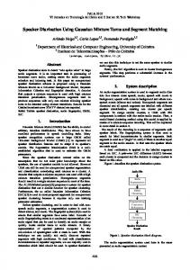
Spk A. Spk B. Input. Figure 1: The output of a speaker diarization system separates the input stream by speaker and non-speech (NSP). Speaker diarization is a ...
Multimodal Speaker Diarization Using Oriented Optical Flow Histograms Mary Tai Knox1,2 , Gerald Friedland1 1
2
International Computer Science Institute, Berkeley, California, USA Department of Electrical Engineering and Computer Sciences, University of California, Berkeley {knoxm, fractor}@icsi.berkeley.edu
Abstract Speaker diarization is the task of partitioning an input stream into speaker homogeneous regions, or in other words, to determine ”who spoke when.” While approaches to this problem have traditionally relied entirely on the audio stream, the availability of accompanying video streams in recent diarization corpora has prompted the study of methods based on multimodal audio-visual features. In this work, we propose the use of robust video features based on oriented optical flow histograms. Using the state-of-the art ICSI diarization system, we show that, when combined with standard audio features, these features improve the diarization error rate by 14% percent over an audio-only baseline. Index Terms: multimodal, speaker diarization, optical flow, audio-visual
1. Introduction The goal of speaker diarization is to partition an input stream into speaker homogeneous speech regions, as shown in Figure 1, where the number of speakers as well as the speaker identities are not known a priori. Speaker diarization has many applications, including speaker adaption for automatic speech recognition, audio indexing, and generating “more usable transcriptions of human-human speech ... for both humans and machines” [1]. The latter being the objective of the NIST Rich Transcription (RT) evaluations.
Input
Diarization Engine
Spk B
Spk A NSP
Spk B
Spk C Spk A NSP
Figure 1: The output of a speaker diarization system separates the input stream by speaker and non-speech (NSP).
Speaker diarization is a task that has been investigated within the speech community for over eight years, over which NIST has held eight RT evaluations [1]. Thus far, most diarization work is done using only the audio data. However, with the increasing ease of capturing and storing data, video data has become more readily available and was included for the first time in the most recent NIST RT 2009 evaluation. However, so far audio-visual systems have not improved accuracy over the audio-only baseline in any NIST RT evaluation. Initial work on audio-visual speaker localization focused on scenarios containing only 2 participants [2, 3], which often contained frontal views of the participants [3]. Both [3] and [2] investigated variants of difference frames, used to capture the movement occurring in the video.
More recent audio-visual, or multimodal, speaker diarization work has considered more realistic and subsequently more challenging datasets, which contain more participants and less restrictive scenarios (e.g. participants are free to move around the room). Thus far, a range of video features have been explored. In [4], the authors used video features from difference frames to locate regions where they hypothesized the speaker was. In [5], scale-invariant feature transform (SIFT) features were extracted over face regions and the mutual information was computed for the average acoustic energy and grayscale pixel value variation. In [6], visual focus of attention features were used to determine the current speaker. In [7], compressed domain video features, specifically average motion vectors over skin regions, were used to improve upon an audio-only diarization baseline. In this work, we explore the use of optical flow based features, which to our knowledge have not been investigated in the context of speaker diarization. Similar to difference frames and compressed domain motion vectors, optical flow captures how images change over time. More specifically, the optical flow is an estimation of the 2-D motion field [8]. We derive features from histograms of oriented optical flow. These features are similar to the video features used in [9], which used audiovisual features for speaker verification. Like recent work in audio-visual speaker diarization [4, 5, 6, 7], we focus on a realistic meeting scenario where there are many speakers who were free to move around the room and generally look at the other participants and not the video cameras, resulting in many non-frontal facial views. Due to the lack of frontal facial views, we do not constrain the video features to isolate regions of the face and instead extract optical flow features over the entire frame to capture the participants’ movements throughout the body; thereby taking advantage of motion related to gesturing (which is a descriptor of speech [10]). Furthermore, we use histogram based features and thus there is no dependency on the location of the motion, which we expect to be more robust to a speaker moving from one side of a room to the other during the course of the meeting. We use a multimodal diarization system similar to those presented in [7] and [6] to combine the audio and video modalities and achieved a 14% relative improvement over the audio-only baseline. This paper is outlined as follows: in Section 2 we describe our multimodal speaker diarization system, in Section 3 we provide and discuss the experiments and results, and in Section 4 we give our conclusions as well as areas of future work.
2. System Description Similar to previous work [7, 6], we use the ICSI multi-stream speaker diarization engine to combine the audio and video modalities.
2.1. Audio Features We extract Mel-Frequency Cepstral Coefficients (MFCCs) to describe the audio data. We compute the first 19 MFCCs, which are computed over a 30 ms window with a 10 ms forward shift. The MFCC features are extracted using the Hidden Markov Model Toolkit (HTK) [11]. Since most speaker diarization systems include MFCCs as their primary features, a system trained on MFCC features alone is used as a baseline.
of the audio features, the video features are repeated 4 times. Table 1: Method used to bin orientation of optical flow, where θ denotes the optical flow orientation, as explained in Section 2.2.2. Bin Horizontal
2.2. Video Features
Diagonal
2.2.1. Optical Flow Preliminary Experiment
Vertical
We initially performed a simple, deterministic experiment to see if the person speaking in a given frame was in fact the most active person as determined by the optical flow. We used OpenCV to compute the Lucas-Kanade optical flow [12] over a 5x5 region for each 160x120 closeup recording of each of the four speakers (sample images from the closeup cameras are shown in Figure 4 and the data is further described in Section 3.1) and then summed the magnitudes of the optical flow for each frame of the closeup video recordings. For each frame of speech, we hypothesized the speaker to be the participant assigned to the closeup view with the greatest amount of optical flow. Using this simple method of determining the speaker, we were correct 53.5% of the time. This result was promising especially considering there were four potential speakers. Moreover, each decision was done at the frame level and no smoothing was applied to ensure sequential speech frames were assigned to the same speaker. Based on the success of this initial experiment, we looked into exploring an optical flow based feature, specifically normalized weighted optical flow histograms which will be described below. 2.2.2. Video Feature Description Since the optical flow seemed promising from the preliminary experiment, we compute a normalized weighted histogram of the optical flow. By computing the histogram, we capture more characteristics of the optical flow without constraining the features to be location dependent. The orientation, θ, is determined by θ = tan−1 (v/u), where u is the optical flow along the xaxis and v is the optical flow along the y-axis. The orientation is then binned according to the conditions given in Table 1, where the weight is given by the log-magnitude of the optical flow. The orientation binning was chosen so that left and right movement would be grouped together as horizontal movement, up and down movement would be grouped as vertical movement, and diagonal movements would similarly be grouped together. Based on this binning, each of the three types of movement contains one third of the possible optical flow orientations. Since the sum of the optical flow is such a valuable descriptor for speech, we chose to bin based on the log-magnitude of the optical flow; thereby giving more weight to regions containing a greater amount of motion. We clip the optical flow magnitude to suppress the effect of erroneous optical flow values and found that binning with a weight of the log-magnitude performed better than the magnitude. Finally, we normalize the 3 bins by the total optical flow log-magnitude; thereby retaining the percent each bin type had of the total optical flow. We also include the normalization factor since the total magnitude of the optical flow has already been shown to be a valuable descriptor of who was speaking. The video used in this work is sampled at 25 Hz while the audio features are sampled at 100 Hz. In order to match the rate
Condition −π/6 ≤ θ < π/6, 5π/6 ≤ θ < 7π/6 π/6 ≤ θ < π/3, 2π/3 ≤ θ < 5π/6, −5π/6 ≤ θ < −2π/3, −π/3 ≤ θ < −π/6 π/3 ≤ θ < 2π/3, −2π/3 ≤ θ < −π/3
2.3. Multi-Stream Diarization Engine The diarization engine used in this study has been used in previous multimodal speaker diarization work [7, 6] and is based on the state-of-the-art ICSI diarization system, which is described in more detail in [13]. The system performs three main tasks: speech/non-speech detection, speaker segmentation, and speaker clustering, where the latter two tasks are performed iteratively using an agglomerative clustering approach. An overview of the system is shown in Figure 2. The system first separates the speech and non-speech regions. Typically this is done using Gaussian Mixture Models (GMMs) as described in [13]. However, in our experiments we use the reference speech/non-speech to isolate the impact of using the video features. The speech regions are then evaluated further for segmentation and speaker assignment using a Hidden Markov Model (HMM) where each state is modeled as a GMM with a minimum duration constraint of 2.5 seconds. We initially choose K clusters, where the number of clusters is equal to the number of HMM states. K is chosen to be much greater than the number of speakers. The GMM parameters are initialized after segmenting the data into K uniform regions. Re-segmentation is performed using Viterbi decoding and the GMMs are retrained based on the new segmentation. The clusters are merged based on the Bayesian Information Criterion (BIC), shown in Equation (1). More specifically, the two clusters which satisfy Equation (1) and have the largest difference between the left and right sides of Equation (1) are merged. In this system, when two clusters are merged the number of parameters for the new cluster is equal to the sum of the parameters in the clusters that are merged which results in the simplified BIC equation shown below. log p(D|θ) > log p(D1 |θ1 ) + log p(D2 |θ2 ),
(1)
where D1 and D2 are the data from clusters 1 and 2, D is the data from D1 ∪ D2 , and θ represents the parameters for the respective models [14]. After two clusters are merged, we repeat the process of retraining the GMMs, re-segmenting the data, and determining which clusters to merge (assuming Equation (1) was satisfied), as shown in Figure 2. Once no two clusters satisfy Equation (1), we output the final segmentation. Similar to [7] and [6], separate GMMs are trained for the audio and video features and the combined log-likelihood of the two streams is defined as
log p(DAU D , DV ID |θi )=(1 ˙ − α) log p(DAU D |θi,AU D ) + α log p(DV ID |θi,V ID ), (2)
where θi,AU D and θi,V ID denote the parameters of the GMM trained on audio features and video features of cluster i, respectively. The combined log-likelihoods are used for segmentation as well as computing the BIC scores. Audio
Speech/Nonspeech Detection Audio Video (speech only) (speech only)
Figure 3: The floor plan of the meeting room including the views from the different camera angles. Figure taken from [16].
Initialization (K Clusters)
vant to gesturing. Audio data was also recorded using multiple nearfield and farfield microphones. In this work, we extract audio features over one farfield microphone. For each of the meetings, speech, as well as other phenomena including dialog acts and head movement, were human annotated.
Re-training & Re-alignment
Merge Clusters?
Yes
No
End (N < K Clusters)
Figure 4: Screenshots from the closeup view in our dataset.
Figure 2: Overview of the multimodal speaker diarization system that uses both audio and video features.
3. Experiments and Results 3.1. Evaluation Data We evaluated our system on twelve meetings from the publicly available Augmented Multi-Party Interaction (AMI) corpus [15], which is the same subset of meetings used in [7, 6]. Each of the twelve meetings consists of four participants that were assigned roles (including project manager, marketing director, industrial designer, and interface designer) in order to develop a prototype of a new remote control over multiple meetings over the course of a day. Though the scenario is fictitious, the meetings are unscripted and otherwise natural. The meetings are on average 27 minutes long. The meetings were recorded in an instrumented meeting room, as shown in Figure 3, with multiple microphones and cameras. Three camera angles were recorded: a closeup view where the cameras were positioned in the center of the table facing each of the four participants, a side view which typically captured two participants sitting on the same side of the table, and a rear view which captured all participants in the meeting. Figures 4 and 5 show sample frames from each of the camera angles. For this study, we used the four closeup camera recordings. Since we plan to carry out experiments on the farfield cameras in the future and frontal faces are generally not visible from the rear camera, we avoided using face specific features and instead hoped to capture face and body movement rele-
Figure 5: Screenshots from the left sideview, rear, and right sideview in our dataset.
3.2. Error Metric The Diarization Error Rate (DER) defined by NIST [1] is used to evaluate the performance of the speaker diarization system. In order to compute the DER, first an optimal one-to-one mapping of reference speakers to system output speakers is determined. The DER is then the sum of the per speaker false alarm time (non-speech that the system identified as speech), miss time (speech that the system identified as non-speech or overlap time in which only one speaker was identified), and speaker error time (assigning an incorrect speaker to a speech segment) divided by the total speech time in an audio file, as shown in Equation (3). DER =
TF A + TM ISS + TSP K TSP EECH
(3)
3.3. Results We first evaluated the baseline system, which used only MFCCs as an input. The number of initial clusters, K, was set to 16 and the original number of mixtures for each state was 5. These were the same parameters used in [7, 6] for their audio-only systems. We then compared the baseline results to that of our multimodal system. The multimodal system combined the audio and video systems, where the audio features were MFCCs and the video features were the total log-magnitude optical flow and normalized weighted oriented optical flow histograms for each closeup video. The number of mixtures for MFCCs was kept at 5, the number of mixtures for the oriented optical flow histograms was 10, and α from Equation (2) was set to 0.1. These values were empirically found to do well for our dataset and are similar to the values used in [7] and [6]. The DERs for the baseline and multimodal systems are shown in Table 2. Note that we have presented both the time weighted DER of all of the meetings, where longer meetings account for more of the total time, similar to what was presented in [6] as well as the average DER for all of the meetings, which weights each meeting equally, and is similar to what was presented in [7]. Table 2: Diarization Error Rates (%) For Baseline and Multimodal Systems and the Relative Improvement (%). Meeting ID IS1000a IS1001a IS1001b IS1001c IS1003b IS1003d IS1006b IS1006d IS1008a IS1008b IS1008c IS1008d Time Avg Meeting Avg
Baseline DER 29.1 30.4 35.6 30.7 16.0 55.2 22.9 56.5 3.1 7.5 12.7 31.9 29.4 27.6
Multimodal DER 29.8 32.1 34.9 26.9 15.2 47.4 16.5 52.4 4.8 7.2 12.4 11.2 25.3 24.2
Relative Improve -2.3 -5.9 2.1 12.4 5.1 14.1 27.9 7.2 -54.3 4.0 2.1 64.8 13.9 12.3
4. Conclusions and Future Work From Table 2, it is clear that the addition of the weighted oriented optical flow histogram features improved the diarization error rate over the baseline system. Although some meetings did not improve, the relative improvement over all 12 meetings was 13.9%. These results are better than the best results presented in [7] and [6]. The multimodal result in [7] was 25.31% DER when averaged across all of the meetings and weighting each meeting equally. We were able to achieve a 24.2% DER when using that metric. However, our audio-only baseline system performed 5% better (absolute) than the one presented in [7] so it is difficult to identify which differences in the systems resulted in the overall improvement. The best result reported in [6] was 26.5% DER, where the total DER was weighted by duration of each meeting. While our work resulted in a 25.3% DER, the speech/non-speech detectors were not the same between the two systems, so again it is difficult to pinpoint what caused the improvement. Nevertheless, it is clear that the use of optical flow based features improved diarization results over an
audio-only baseline. In the future we plan to investigate how the normalized weighted oriented optical flow histogram features fare in the rear camera setting. In order to do so, we must first reliably track the participants throughout the meeting. We also would like to more closely investigate the video features to see how they would perform in speech/non-speech detection as this is an area of improvement for speaker diarization systems and would give us more insight into useful features.
5. References [1] NIST, “The 2009 (RT-09) rich transcription meeting recognition evaluation plan,” 2009. [2] H. Vajaria, T. Islam, S. Sarkar, R. Sankar, and R. Kasturi, “Audio segmentation and speaker localization in meeting video,” in Proceedings of the 18th International Conference on Pattern Recognition, vol. 2, 2006, pp. 1150–1153. [3] H. Nock, G. Iyengar, and C. Neti, “Speaker localisation using audio-visual synchrony: An empirical study,” in Proceedings of the 10th ACM International Conference on Multimedia, 2003. [4] H. Vajaria, S. Sarkar, R. Sankar, and R. Kasturi, “Exploring cooccurence between speech and body movement for audio-guided video localization,” in IEEE Transactions on Circuits and Systems for Video Technology, vol. 18, 2008, pp. 1608–1617. [5] A. Noulas, G. Englebienne, and B. Krose, “Multimodal speaker diarization,” in Computer Vision and Image Understanding, 2009. [6] G. Garau, S. Ba, H. Bourlard, and J. Odobez, “Investigating the use of visual focus of attention for audio-visual speaker diarisation,” in ACM Multimedia, 2009. [7] G. Friedland, H. Hung, and C. Yeo, “Multi-modal speaker diarization of real-world meetings using compressed-domain video features,” Proc. IEEE ICASSP, 2009. [8] J. Barron, D. Fleet, and S. Beauchemin, “Performance of optical flow techniques,” in International Journal of Computer Vision, 1994, pp. 43–77. [9] C. Bregler, G. Williams, S. Rosenthal, and I. McDowall, “Improving acoustic speaker verification with visual body-language features,” in Proc. IEEE ICASSP, 2009. [10] D. McNeill, Language and Gesture. New York: Cambridge University Press, 2000. [11] “Hidden markov model toolkit (HTK),” http://htk.eng.cam.ac.uk/. [12] B. Lucas and T. Kanade, “An iterative image registration technique with an application to stereo vision,” in Proceedings of Imaging Understanding Workshop, 1981, pp. 121–130. [13] C. Wooters and M. Huijbregts, “The icsi rt07s speaker diarization system,” in Proceedings of the RT07 Meeting Recognition Evaluation Workshop, 2007. [14] J. Ajmera and C. Wooters, “A robust speaker clustering algorithm,” in Proceedings of IEEE Speech Recognition and Understanding Workshop, St. Thomas, US Virgin Islands, 2003. [15] J. Carletta, S. Ashby, S. Bourban, M. Flynn, M. Guillemot, T. Hain, J. Kadlec, V. Karaiskos, W. Kraaij, M. Kronenthal, G. Lathoud, M. Lincoln, A. Lisowska, I. McCowan, W. Post, D. Reidsma, and P. Wellner, “The AMI meetings corpus,” in Proceedings of the Measuring Behavior 2005 Symposium on Annotating and Measuring Meeting Behavior, 2005. [16] H. Hung, Y. Huang, G. Friedland, and D. Gatica-Perez, “Estimating the dominant person in multi-party conversations using speaker diarization strategies,” in Proc. IEEE ICASSP, 2008.