(LDSs) and perform classification using metrics on the space of LDSs, e.g. Binet-Cauchy kernels. However, such approaches are only applicable to time series ...
Histograms of Oriented Optical Flow and Binet-Cauchy Kernels on Nonlinear Dynamical Systems for the Recognition of Human Actions Rizwan Chaudhry, Avinash Ravichandran, Gregory Hager and Ren´e Vidal Center for Imaging Science, Johns Hopkins University 3400 N Charles St, Baltimore, MD 21218
Abstract System theoretic approaches to action recognition model the dynamics of a scene with linear dynamical systems (LDSs) and perform classification using metrics on the space of LDSs, e.g. Binet-Cauchy kernels. However, such approaches are only applicable to time series data living in a Euclidean space, e.g. joint trajectories extracted from motion capture data or feature point trajectories extracted from video. Much of the success of recent object recognition techniques relies on the use of more complex feature descriptors, such as SIFT descriptors or HOG descriptors, which are essentially histograms. Since histograms live in a non-Euclidean space, we can no longer model their temporal evolution with LDSs, nor can we classify them using a metric for LDSs. In this paper, we propose to represent each frame of a video using a histogram of oriented optical flow (HOOF) and to recognize human actions by classifying HOOF time-series. For this purpose, we propose a generalization of the Binet-Cauchy kernels to nonlinear dynamical systems (NLDS) whose output lives in a non-Euclidean space, e.g. the space of histograms. This can be achieved by using kernels defined on the original non-Euclidean space, leading to a well-defined metric for NLDSs. We use these kernels for the classification of actions in video sequences using (HOOF) as the output of the NLDS. We evaluate our approach to recognition of human actions in several scenarios and achieve encouraging results.
1. Introduction Analysis of human activities has always remained a topic of great interest in computer vision. It is seen as a stepping stone for applications such as automatic environment surveillance, assisted living and human computer interaction. The surveys by Gavrila [14], Aggarwal et al. [1] and by Moeslund et al., [18], [19] provide a broad overview of over three hundred papers and numerous approaches for analyzing human motion in videos, including human motion
capture, tracking, segmentation and recognition. Related work. Recent work on activity recognition can be broadly classified into three types of approaches: local, global and system-theoretic. Local approaches use local spatiotemporal features, e.g. [17, 10, 30] to represent human activity in a video. Niebles [20] presented an unsupervised method similar to the bagof-words approach for learning the probability distributions of space-time interest points in human action videos. ˙Ikizler et al. [16] presented a method whereby limb motion model units are learnt from labeled motion capture data and used to detect more complex unseen motions in a test video using search queries specific to the limb motion in the desired activity. However, an important limitation of the aforementioned approaches is that they do not incorporate global characteristics of the activity as a whole. Global approaches use global features such as optical flow to represent the state of motion in the whole frame at a time instant. With static background, one can represent the type of motion of the foreground object by computing features from the optical flow. In [13], optical flow histograms were used to match the motion of a player in a soccer match to that of a subject in a control video. Tran et al. in [27] present an optical flow and shape based approach that uses separate histograms for the horizontal and vertical components of the optical flow as well as the silhouette of the person as a motion descriptor. [15] and [31] represent human activities by 3-D space-time shapes. Classification is performed by comparing geometric properties of these shapes against training data. All these approaches, however, do not model the characteristic temporal dynamics of human activities. Moreover, comparison is done either on a frameby-frame basis or by using other ad-hoc methods. Clearly, the natural way to compare human activities is to compare the temporal evolution of global features as a whole. System-theoretic approaches to recognition of human actions model feature variations with dynamical systems and hence specifically consider the dynamics of the activity. The recognition pipeline is composed of 1) finding features in every frame, 2) modeling the temporal evolution of these
1
1
1
1
1
1
0.9
0.9
0.9
0.9
0.9
0.9
0.8
0.8
0.8
0.8
0.8
0.8
0.7
0.7
0.7
0.7
0.7
0.7
0.6
0.6
0.6
0.6
0.6
0.6
0.5
0.5
0.5
0.5
0.5
0.5
0.4
0.4
0.4
0.4
0.4
0.4
0.3
0.3
0.3
0.3
0.3
0.3
0.2
0.2
0.2
0.2
0.2
0.2
0.1
0.1
0.1
0.1
0.1
0.1
0
0
0
0
0
0
Figure 1. Optical flows and HOOF feature trajectories
features with a dynamical system, 3) using a similarity criteria, e.g. distances or kernels between dynamical systems, to train classifiers, and 4) using them on novel video sequences. Bissacco et al. used joint-angle trajectotries in [3] as well as joint trajectories from motion-capture data and features extracted from silhouettes in [4] to represent the action profiles. Ali et al. in [2] used joint trajectories to extract invariant features to model the non-linear dynamics of human activities. However, these approaches are mostly limited to local feature representations and to our knowledge, there has been no work on modeling the dynamics of global features, e.g. optical flow variations. Paper contributions. In this paper, we propose the Histogram of Oriented Optical Flow (HOOF) features to represent human activities. These novel features are independent of the scale of the moving person as well as the direction of motion. Extraction of HOOF features does not require any prior human segmentation or background subtraction. However, HOOF features are non-Euclidean, and thus the evolution of HOOF features creates a trajectory on a nonlinear manifold. Traditionally, Linear Dynamical Systems (LDSs) have been used to model feature time series that are Euclidean, e.g. joint angles, joint trajectories, pixel intensities, etc. Non-Euclidean data like histogram time series need to be modeled with Non-Linear Dynamical Systems (NLDS). Hence, similarity criteria designed for LDSs cannot be used to compare two histogram time series. In this paper, we extend the Binet-Cauchy kernels [29] to NLDS. This is done by replacing an infinite sum of output feature inner products in the kernel expression by a Mercer kernel [23] on the output space. We model the proposed HOOF features as outputs of NLDS and use the Binet-Cauchy kernels for NLDS to perform human activity recognition on the Weizmann database [15] with encouraging results.
Paper outline. The rest of this paper is organized as follows. §2 briefly reviews the LDS recognition pipeline for Euclidean time-series data. §3 proposes the Histogram of Oriented Optical Flow (HOOF) features, which are used to model the activity profile in each frame of a video. Every activity video is thus represented as a non-Euclidean time-series of HOOF features. §4 introduces NLDS and describes how NLDS parameters can be learnt using kernels defined on the underlying non-Euclidean space. §5 presents the Binet-Cauchy kernels for NLDSs which define a similarity metric between two non-Euclidean time-series. §6 gives experimental results for human activity recognition using the proposed metric and features. Finally, §7 gives concluding remarks and future directions.
2. Recognition with Linear Dynamical Systems A LDS is represented by the tuple M = (µ, x0 , A, C, B, R) and evolves in time according to the following equations � xt+1 = Axt + Bvt . (1) yt = µ + Cxt + wt Here xt ∈ Rn is the state of the LDS at time t; yt ∈ Rp is the observed output or feature at time t; x0 is the initial state N −1 of the system; and µ ∈ Rp is the mean of {yt }t=0 , e.g. the n×n mean joint angle configuration, etc. A ∈ R describes the dynamics of the state evolution, B ∈ Rn×nv models the way in which input noise affects the state evolution and C ∈ Rp×n transforms the state to an output or observation of the overall system. vt ∈ Rnv and wt ∈ Rp are the system noise and the observation noise at time t, respectively. We assume that the noise processes are zero-mean i.i.d. Gaussian, such that vt ∼ G(vt , 0, Inv ) and wt ∼ G(wt , 0, R), R ∈ Rp×p ,
where G(z, µz , Σ) = (2π)−n/2 |Σ|−1/2 exp(− 12 kz − µz k2Σ ) is a multivariate Gaussian distribution on z with kzk2Σ = z> Σ−1 z. By this definition, Bvt ∼ G(Bvt , 0, Q) where Q = BB > ∈ Rnv ×nv . We also assume that vt and wt are independent processes. Given a set of T training videos, the first task is to learn the parameters Mi , i = 1, . . . , T , from the feature trajectories of each video. There are several methods to learn these system parameters, e.g. [25], [28] and [11]. Once these parameters are identified for each of the videos, various metrics can be used to define the similarity between these LDSs. In particular, three major types of metrics are 1) geometric distances based on subspace angles between the observability subspaces of the LDSs [9], 2) algebraic metrics like the Binet-Cauchy kernels [29] and 3) information theoretic metrics like the KL-divergence [6]. Given a metric, all pairwise similarities are evaluated on the training data and used for classification of novel sequences using methods such as k-Nearest Neighbors (kNN) or Support Vector Machine (SVM).
To overcome these issues, in this paper we propose the Histogram of Oriented Optical Flow (HOOF), which is defined as follows. First, optical flow is computed at every frame of the video. Each flow vector is binned according to its primary angle from the horizontal axis and weighted according to its magnitude. Thus, all optical flow vectors, v = [x, y]> with direction, θ = tan−1 ( xy ) in the range b−1 π b π +π ≤θ at each time instant t. In order
to use such histograms for recognition purposes, we need to have a way of comparing two histograms. To that end, notice that histograms cannot be treated as simple vectors in a Euclidean space. Histograms are essentially probability mass functions, hence they must satisfy the constraints B X ht;i = 1 and ht;i ≥ 0, ∀i ∈ {1, . . . , B}. At first sight,
hypersphere or SB−1 . The Riemannian metric between two points R1 and R2 on the hypersphere is d(R1 , R2 ) = cos−1 (R1> R2 ). Thus a kernel between two histograms can be defined as an inner product on their square root representations: B X p kS (h1 , h2 ) = h1;i h2;i . (3) i=1
i=1
one may think that this space is still simple enough. However, the space of histograms H is actually a Riemannian manifold with a nontrivial structure. The problem of equipping the space of probability density functions (PDFs) with a differential manifold structure and defining a Riemannian metric on it has been an active area of research in the field of information geometry. The work by Rao [21] was the first to introduce a Riemannian structure to this statistical manifold by introducing the Fisher-Rao metric. The Fisher-Rao metric, however, is extremely hard to work with due to the difficulty in computing geodesics on this space [26]. Even though the space H turns out to be difficult to work with, we know that it is not the only possible representation for PDFs. There are many different re-parameterizations of PDFs that are equivalent. These include the cumulative distribution function, log density function and square-root density function. Each of these parameterizations will lead to a different resulting manifold. Depending on the choice of representation, the resulting Riemannian structure can have varying degrees of complexity and numerical techniques may be required to compute geodesics on the manifold. For the sake of computational simplicity, in this paper we will restrict our attention to similarity measures built by mapping the histogram h ∈ H to a high dimensional (possibly infinite) Hilbert space, F, using the map Φ : H → F. Since F is a Hilbert space, all the natural notions of finding distances between two points can be employed for comparison. Most of the time, however, the map Φ cannot be found. Mercer kernels [23] have the special property of being positive definite kernels that induce an inner product in a higher dimensional spaceunder the map Φ. This space is called the Reproducing Kernel Hilbert Space (RKHS) for the kernel. More specifically, for points lying on the non-linear manifold H, the Mercer kernel is given by k(h1 , h2 ) = Φ(h1 )> Φ(h2 ) and hence a similarity measure on the RKHS can be computed by simply computing the kernel function on the original representation without knowing the mapping Φ. We now briefly describe some popular kernel measures used on the space of histograms. The histogram, ht = [ht;1 , . . . , ht;B ] can be reparameterized to the square root representation for histograms, B X p p p √ ht := [ ht;1 , . . . , ht;B ] such that ( ht;i )2 = 1. i=1
This projects every histogram onto the unit B-dimensional
Note that this is precisely the kernel that can be achieved by using the RBF kernel, k(h1 , h2 ) = exp(−d(h1 , h2 )), on the Bhattacharya distance between the two histograms. Minimum Difference of Pairwise Assignment (MDPA) [5] is similar to the Earth Mover’s Distance (EMD) [22] and is a metric on the space of histograms that implicitly is a summation of distances between points on an underlying metric space from which the histograms were created. For ordinal histograms, i.e., histograms created from linearly varying data (as opposed to modular data, e.g. the modu. lar group Zp = {0, 1, . . . , p − 1}), the MDPA distance is B X X i (h1;j − h2;j ) . dMDPA (h1 , h2 ) = (4) i=1 j=1 Another popular distance between two histograms is the χ2 distance which is defined as B
dχ2 (h1 , h2 ) =
1 X |h1;i − h2;i | 2 i=1 h1;i + h2;i
2
(5)
We can use the RBF kernel to create kernels as similarity measures from these distances. Finally, the Histogram Intersection Kernel (HIST) [12] is another Mercer kernel [23] on the space of histograms and is defined for normalized histograms as kHIST =
B X
min(h1;i , h2;i ).
(6)
i=1
The inner product of the square-root representations is by construction an inner product and hence is a Mercer kernel. Also, the χ2 and HIST kernels are provably Mercer kernels [32], [12]. However, to the best of our knowledge, the positive-definiteness of the MDPA kernel has not been established [32].
3.2. Kernels for comparing HOOF time series Since HOOF features ht = [ht;1 , ht;2 , . . . , ht;B ]> are defined at each frame of the video, our actual representa−1 tion is a time series of these histograms {ht }N t=0 . Our goal is to compare these time series in order to perform classification of actions. But rather than comparing these time series directly, we want to exploit the temporal evolution of these histograms in order to distinguish different actions.
We posit that each action induces a time-series of HOOF with specific dynamics, and that different actions induce different dynamics. Therefore, we propose to recognize actions by comparing the dynamics of HOOF time series. There are two important technical challenges in developing a framework for the classification of HOOF time series. The first one is that, because each histogram ht lives in a non-Euclidean space H, we cannot model its temporal evolution with LDSs. We address this issue in §4 by using the previously defined kernels in H to define a NLDS. The second challenge is how to compute a distance between HOOF time series. We address this issue in §5, where we extend Binet-Cauchy kernels to NLDSs.
4. Modeling HOOF Time Series with NonLinear Dynamical Systems Modeling Euclidean feature trajectories with LDSs has been very useful for dynamical system recognition. However we need NLDSs to model non-Euclidean feature trajectories like histograms. Consider the Mercer kernel, k(yt , yt0 ) = Φ(yt )> Φ(yt0 ) on the non-Euclidean space such that the implicit map, Φ, maps the original non-Euclidean space H to an RKHS. We can therefore transform the non-Euclidean features, −1 N −1 {yt }N t=0 , to features in the RKHS{Φ(yt )}t=0 and assume that the transformed trajectories follow a linear dynamical system � xt+1 = Axt + Bvt (7) Φ(yt ) = Cxt + wt The main difference between (7) and (1) is that we do not necessarily know the embedding Φ, hence we cannot identify (A, C) as before. Moreover, even if we knew Φ, C : Rn → F is now a linear operator, rather than simply a matrix, because F is possibly infinite dimensional. Therefore, the goal is to identify the parameters (A, B), the sequence xt , and some representation for C by exploiting the fact that we only know the kernel k. In [7], an approach based on Kernel PCA (KPCA) [24] that parallels the PCA approach for learning LDS parameters in [11] was proposed to learn the system parameters for equation N −1 (7). Briefly, given the output feature sequence, {yt }t=0 , N −1 the intra-sequence kernel matrix, K = {k(yi , yj )}i,j=0 is computed, where k(yi , yj ) = Φ(yi )> Φ(yj ). The centered kernel matrix, that represents the kernel between zero-mean data in the high-dimensional space, is thus computed as ˜ = (I − 1 ee> )K(I − 1 ee> ) where e = [1, . . . , 1]> ∈ K N N ˜ = RN . After performing the eigenvalue decomposition K > V DV , the j-th eigenvector vj can be used to obtain the N X j-th kernel principal component as αi,j Φ(yi ), where i=1
αi,j represents the i-th component of the j-th weight vector,
αj = √1 vj , assuming that the eigenvectors are sorted in λj
descending order of the eigenvalues {λj }N j=1 . ˜ Given α and K, the sequence of hidden states X = [x0 , x1 , . . . , xN −1 ] and the state-transition matrix, A, can be estimated as X A
˜ = α> K =
(8) †
[x1 , x2 , . . . , xN −1 ][x0 , x1 , . . . , xN −2 ]
(9)
ˆ t = xt − xt−1 , The state noise at time t is estimated as v PN −1 ˆtv ˆ t> . and the noise covariance matrix as Q = N 1−1 i=1 v Using a Cholesky decomposition on Q, B is estimated as BB > = Q. For details on estimating R and other parameters, refer to [7]. Notice, however, that we have not shown how to estimate C or a representation of it, though it is clear that C ˜ is somehow implicitly represented by the kernel matrix K. Since our goal is to use the NLDS in (7) for recognition, rather than synthesis, we do not actually need to compute C. All we need is a way of comparing two linear operators C, which can be done by comparing the corresponding ˜ as we show in the next section. kernel matrices K,
5. Comparing HOOF Time Series with BinetCauchy Kernels for NLDS Vishwanathan et al. [29] presented the family of BinetCauchy kernels for LDSs. In this section we briefly review the main concepts of the Binet-Cauchy kernels for LDSs and then develop extensions for the case of NLDSs. From the family of Binet-Cauchy kernels, the trace T kernel, KLDS , for comparing two infinitely long zeromean Euclidean time-series generated by the LDSs M = (x0 , A, C, B, R), and M0 = (x00 , A0 , C 0 , B 0 , R0 ) is defined as T 0 ∞ T 0 KLDS ({yt }∞ t=0 , {yt }t=0 ) = KLDS (M, M ) "∞ # X := Ev,w λt yt> yt0 .
(10)
t=0
Here 0 < λ < 1 and E represents the expected value of the infinite sum of the inner products w.r.t. the joint probability distribution of vt and wt . It was shown in [29] that if the two LDSs have the same underlying and independent noise processes, with covariances Q and R for the state and output, respectively, then the Binet-Cauchy trace kernel can be computed in closed form as T 0 KLDS (M1 , M2 ) = x> 0 P x0 +
where P =
∞ X t=0
λ trace(QP + R), 1−λ
λt (At )> C > C 0 A0
t
(11)
(12)
If λ|||A||| |||A0 ||| < 1, where |||.||| is a matrix norm, then P can be computed by solving the Sylvester equation [29], P = λA> P A0 + C > C 0 .
(13)
Notice that as a result of the system parameter learning method [11], the second term on the right side of equation (13), C > C 0 , is the matrix of all pairwise inner products of ¯ , y1 − the principal components of the matrix Y = [y0 − y ¯ , . . . , yN −1 − y ¯ ] and the matrix Y 0 = [y00 − y ¯ 0 , y10 − y 0 ¯ 0 , . . . , yN ¯ 0 ], where y ¯ is the mean of the sequence y 0 −1 − y N −1 {yt }t=0 and so on. Hence, the (i, j)-th entry of C > C 0 is 0 0 c> i cj , where ci is the i-th principal component of Y and cj 0 is the j-th principal component of Y . We now develop the Binet-Cauchy trace kernel for NLDSs. From equation (10), we see that the Binet-Cauchy trace kernel for LDSs is the expected value of an infinite series of weighted inner products between the outputs of two systems. We can similarly write the Binet-Cauchy trace kernel for NLDSs as the expected value of an infinite series of weighted inner products between the outputs after embedding them into the high-dimensional (possibly infinite) space using the map Φ. Specifically, "∞ # X T 0 t > 0 KNLDS (M, M ) := Ev,w λ Φ(yt ) Φ(yt ) " = Ev,w
t=0 ∞ X
# t
λ
k(yt , yt0 )
,
(14)
t=0
where k is the kernel defined on the non-Euclidean space of outputs H. If we look at equation (13), we see that in the case of NLDSs the equivalent form for the trace kernel is not immediately obtainable, because C and C 0 are unknown, and hence the term C > C 0 cannot be evaluated directly. However, notice that C > C 0 is now the product of the matrices formed from the kernel principal components from the NLDS identification process as opposed to the principal components as in the case of LDSs. Thus, similar to the approach used in [7], the (i, j)-th entry of C > C 0 can be computed as [C > C 0 ]i,j = vi> vj0 "N #> N 0 X X 0 0 = αk,i Φ(yk ) αl,j Φ(yl ) k=1
=
αi> Sαj0
l=1
(15)
where S is the matrix of all inner products of the form [Φ(yk )> Φ(yl0 )]k,l = [k(yk , yl0 )]k,l , where k ∈ {1, . . . , N }, l ∈ {1, . . . , N 0 }. Before computing the entries of C > C 0 in equation (15), we need to center the kernel com-
putation S. This is done by computing, α ˜ i = αi −
e> αi e N
e> αj0 e and evaluating, F = α ˜ > S α˜0 N0 Hence, the Binet-Cauchy kernel for NLDS requires the computation of the infinite sum,
and α ˜ j0 = αj0 −
P¯ =
∞ X
t
λt (At )> F A0 ,
(16)
t=0
If λ|||A||| |||A0 ||| < 1, where |||.||| is a matrix norm, then P¯ can be computed by solving the corresponding Sylvester equation: P¯ = λA> P¯ A0 + F (17) and the Binet-Cauchy trace kernel for NLDS is T ¯ > KNLDS (M1 , M2 ) = x> 0 P x0 +
λ trace(QP¯ +R) (18) 1−λ
Notice that equation (18) is a general kernel that takes into consideration the dynamics of the system encoded by (A, C), the noise processes, Q and R, and the initial state, x0 . The effect of the initial state in a periodic time series is to simply delay the time series. Since in activity recognition it does not matter, e.g., at which part of the walking cycle the video begins, we would like a kernel that is independent of the initial states and the noise processes. Hence we define the Binet-Cauchy maximum singular value kernel for NLDS as σ KNLDS = max σ(P¯ ) (19) which is the maximum singular value of P¯ and is a kernel only on the dynamics of the NLDS. Furthermore, we can show that the Martin distance used by [7] (and all subspace angles based distances between dynamical systems) are special cases of the Binet-Cauchy kernels [8].
6. Experiments To test the performance of our proposed HOOF features on activity recognition using the Binet-Cauchy kernel for NLDS, we perform a number of experiments on the Weizmann Human Action dataset [15]. This dataset contains 94 videos of 10 different actions each performed by 9 different persons. The classes of actions include running, side walking, waving, jumping, etc. Optical flow was computed using OpenCV on each of the sequences and HOOF histograms were extracted from each frame leading to a HOOF time series for each video sequence.
6.1. Classification Results We use each of the kernels described in section §3.1 to perform Kernel PCA on the HOOF time series extracted
Recognition with distance between HOOF temporal means
0.6 0.55 0.5
0.4 0.35 Error rate
0.4 Error rate
Martin Max SV kernel Temp Means
0.45
0.45
0.35 0.3
0.3 0.25 0.2
0.25
0.15
0.2
0.1
0.15 0.1
Geodesic kernel
0.5
Euclidean Geodesic MDPA chi−square Non−intersection
0
10
20
30
40 50 60 Number of bins
70
80
90
100
Figure 3. Misclassification rates when using distances between HOOF means
from each video. We then use the Binet-Cauchy maxiσ mum singular value kernel, KNLDS , to compute all pairwise similarity values. We normalize the similarity values such that K(M, M0 ) = 1, if M = M 0 by computK(M, M0 ) ing, K 0 (M, M0 ) = p and findK(M, M), K(M0 , M0 ) ing pair-wise distances between systems by computing, d(M, M0 ) = 2(1 − K(M1 , M2 )). Classification is then performed with Leave-one-out, 1-Nearest Neighbor classification using these distance values. As a baseline, Figure 3 shows the performance of using the distance between the temporal means to perform classification. The temporal means werePcomputed by averaging ¯ = 1 N −1 hi . Notice that h ¯ the histogram time-series h i=0 N is also a histogram and we can apply the distance metrics in section §3.1 to compare them. Although using the mean histograms to represent the activity profile ignores any dynamics of the motion, we see that the HOOF features give low error rates. Figure 4 shows the error rates for the inner product of the square root representations, or the Geodesic kernel, across all bin sizes. We can see that the Binet-Cauchy maximum singular value kernel gives the lowest error rate of 5.6% achieving a recognition rate of 94.4%. The corresponding confusion matrix is shown in Figure 5. One sequence each is misclassified for the classes jump and run and three sequences of class wave1 were misclassified as wave2. Table 1 compares the performance of three state of the art activity recognition algorithms on the Weizmann database with similar experimental setups. We can see that the proposed method performs better than two of the methods with any choice of the Mercer kernel on the space of histograms. Furthermore, the proposed method performs almost as well as the best method in [15]. The small decrease in performance is because of the fact that [15] requires the accurate extrac-
0.05
3
13
23
33
43 53 63 Number of bins, b
73
83
93
Figure 4. Misclassification rates with Geodesic kernel on NLDS
Proposed method - Geodesic kernel Proposed method - MDPA distance Proposed method - χ2 distance Proposed method - HIST kernel Gorelick et al. [15] Ali et al. [2] Niebles et al. [20]
94.44 93.44 95.66 92.33 97.83 92.60 90.00
Table 1. Comparison of recognition rates with state of the art methods on the Weizmann database
tion of the silhouette of the moving person at every time instant which is a very strong assumption. Our method, on the other hand, is very general and does not require any preprocessing steps and still gives better results than all stateof-the-art methods, except [15]. Riemannian metric with Binet Cauchy kernel, Leave−one−out 1−NN bend
100
0
0
0
0
0
0
0
0
0
jack
0
100
0
0
0
0
0
0
0
0
jump
0
0
89
0
0
0
11
0
0
0
pjump
0
0
0
100
0
0
0
0
0
0
run
0
0
0
0
89
0
11
0
0
0
side
0
0
0
0
0
100
0
0
0
0
skip
0
0
0
0
0
0
100
0
0
0
walk
0
0
0
0
0
0
0
100
0
0
wave1
0
0
0
0
0
0
0
0
67
33
0
100
wave2
0
0
0
0
0
0
0
0
bend
jack
jump
pjump
run
side
skip
walk
wave1 wave2
Figure 5. Confusion matrix for recognition on Weizmann database, average recognition rate is 94.4%
7. Conclusions and Future Work We have presented an activity recognition method that models the activity in a scene as a time-series of nonEuclidean Histograms of Oriented Optical Flow features. We have shown that these features do not need any preprocessing, human detection, tracking and prior background subtraction and represent the activity comprehensively. The HOOF features are scale-invariant as well as independent of the direction of motion. Since the space of histograms is non-Euclidean, we have modeled the temporal evolution of HOOF features using NLDSs and learnt the system parameters using kernels on the original histograms. More importantly, we have extended the Binet-Cauchy kernels for measuring the similarities between two NLDSs and shown that the Binet-Cauchy kernels can also be computed by evaluating pairwise Mercer kernels on the non-Euclidean space of features. We have applied our framework to our proposed HOOF features and have achieved state of the art results on the Weizmann Human Gait database. Currently we are working on extending our method to multiple disconnected motions in a scene by tracking and segmenting optical flow activity in the scene as well as accounting for the motion of the camera.
8. Acknowledgements This work was partially supported by startup funds from JHU and by grants ONR N00014-05-10836, ONR N0001409-1-0084, NSF CAREER 0447739 and ARL RoboticsCTA 80014MC.
References [1] J. K. Aggarwal and Q. Cai. Human motion analysis: A review. Computer Vision and Image Understanding, 73:90–102, 1999. [2] S. Ali, A. Basharat, and M. Shah. Chaotic invariants for human action recognition. In IEEE International Conference on Computer Vision, 2007. [3] A. Bissacco, A. Chiuso, Y. Ma, and S. Soatto. Recognition of human gaits. In IEEE Conference on Computer Vision and Pattern Recognition, volume 2, pages 52–58, 2001. [4] A. Bissacco, A. Chiuso, and S. Soatto. Classification and recognition of dynamical models: The role of phase, independent components, kernels and optimal transport. IEEE Transactions on Pattern Analysis and Machine Intelligence, 29(11):1958–1972, 2006. [5] S.-H. Cha and S. N. Srihari. On measuring the distance between histograms. Pattern Recognition, 35(6):1355–1370, June 2002. [6] A. Chan and N. Vasconcelos. Probabilistic kernels for the classification of auto-regressive visual processes. In IEEE Conference on Computer Vision and Pattern Recognition, volume 1, pages 846–851, 2005. [7] A. Chan and N. Vasconcelos. Classifying video with kernel dynamic textures. In IEEE Conference on Computer Vision and Pattern Recognition, pages 1–6, 2007. [8] R. Chaudhry and R. Vidal. Supplemental material for “Binet-Cauchy kernels on nonlinear dynamical systems for the recognition of human actions”. Technical Report Vision Lab TR 2009/01, Johns Hopkins University, 2009.
[9] K. D. Cock and B. D. Moor. Subspace angles and distances between ARMA models. System and Control Letters, 46(4):265–270, 2002. [10] P. Doll´ar, V. Rabaud, G. Cottrell, and S. Belongie. Behavior recognition via sparse spatio-temporal features. In VS-PETS, October 2005. [11] G. Doretto, A. Chiuso, Y. Wu, and S. Soatto. Dynamic textures. Int. Journal of Computer Vision, 51(2):91–109, 2003. [12] R. Duda, P. Hart, and D. Stork. Pattern Classification. WileyInterscience, October 2004. [13] A. Efros, A. Berg, G. Mori, and J. Malik. Recognizing action at a distance. In IEEE International Conference on Computer Vision, pages 726–733, 2003. [14] D. M. Gavrila. The visual analysis of human movement: A survey. Computer Vision and Image Understanding, 73:82–98, 1999. [15] L. Gorelick, M. Blank, E. Shechtman, M. Irani, and R. Basri. Actions as space-time shapes. IEEE Trans. on Pattern Analysis and Machine Intelligence, 29(12):2247–2253, 2007. [16] N. ˙Ikizler and D. A. Forsyth. Searching for complex human activities with no visual examples. International Journal of Computer Vision, 80(3):337–357, 2008. [17] I. Laptev. On space-time interest points. Int. Journal of Computer Vision, 64(2-3):107–123, 2005. [18] T. B. Moeslund and E. Granum. A survey of computer vision-based human motion capture. Computer Vision and Image Understanding, 81:231–268, 2001. [19] T. B. Moeslund, A. Hilton, and V. Krger. A survey of advances in vision-based human motion capture and analysis. Computer Vision and Image Understanding, 104:90–126, 2006. [20] J. C. Niebles, H. Wang, and L. Fei-Fei. Unsupervised learning of human action categories using spatial-temporal words. International Journal of Computer Vision, 79:299–318, 2008. [21] C. R. Rao. Information and accuracy attainable in the estimation of statistical parameters. Bull. Calcutta Math Soc., 37:81–89, 1945. [22] Y. Rubner, C. Tomasi, and L. J. Guibas. A metric for distributions with applications to image databases. In IEEE Int. Conf. on Computer Vision, 1998. [23] B. Sch¨olkopf and A. Smola. Learning with Kernels. MIT Press, Cambridge, MA, 2002. [24] B. Scholkopf, A. Smola, and K.-R. Muller. Nonlinear component analysis as a kernel eigenvalue problem. Neural Computation, 10:1299–1319, 1998. [25] R. Shumway and D. Stoffer. An approach to time series smoothing and forecasting using the EM algorithm. Journal of Time Series Analysis, 3(4):253–264, 1982. [26] A. Srivastava, I. Jermyn, and S. Joshi. Riemannian analysis of probability density functions with applications in vision. In IEEE Conference on Computer Vision and Pattern Recognition, 2007. [27] D. Tran and A. Sorokin. Human activity recognition with metric learning. In European Conference on Computer Vision, 2008. [28] P. van Overschee and B. D. Moor. Subspace Identification for Linear Systems. Kluwer Academic Publishers, 1996. [29] S. Vishwanathan, A. Smola, and R. Vidal. Binet-Cauchy kernels on dynamical systems and its application to the analysis of dynamic scenes. International Journal of Computer Vision, 73(1):95–119, 2007. [30] G. Willems, T. Tuytelaars, and L. J. V. Gool. An efficient dense and scale-invariant spatio-temporal interest point detector. In European Conference on Computer Vision, 2008. [31] A. Yilmaz and M. Shah. Actions sketch: A novel action representation. In IEEE Conference on Computer Vision and Pattern Recognition, pages 984–989, 2005. [32] J. Zhang, M. Marszalek, S. Lazebnik, and C. Schmid. Local features and kernels for classification of texture and object categories: An in-depth study. Technical report, INRIA, 2005.