multimodality and multiresolution image fusion - Semantic Scholar

MULTIMODALITY AND MULTIRESOLUTION IMAGE FUSION Paul M. de Zeeuw, Eric J. E. M. Pauwels and Jungong Han Centrum Wiskunde & Informatica, P.O. Box 94079, NL–1090 GB, Amsterdam, The Netherlands {Paul.de.Zeeuw, Eric.Pauwels, J.Han}@cwi.nl

Keywords:

Multimodality, Multiresolution, Image Fusion.

Abstract:

Standard multiresolution image fusion of multimodal images may yield an output image with artifacts due to the occurrence of opposite contrast in the input images. Equal but opposite contrast leads to noisy patches, instable with respect to slight changes in the input images. Unequal and opposite contrast leads to uncertainty of how to interpret the modality of the result. In this paper a biased fusion is proposed to remedy this, where the bias is towards one image, the so-called iconic image, in a preferred spectrum. A nonlinear fusion rule is proposed to prevent that the fused image reverses the local contrasts as seen in the iconic image. The rule involves saliency and a local match measure. The method is demonstrated by artificial and real-life examples.

1

INTRODUCTION

Image fusion seeks to combine images in such a way that all the salient information is put together into (usually) one image suitable for human perception or further processing. One can roughly divide the field into two categories: monomodal and multimodal image fusion. An example of the need for the first can be found in light microscopy where one encounters the problem of limited depth-of-field, i.e. only part of the specimen under consideration will be in focus. By fusing multiple images with different focus one acquires an image which has overall focus. Examples of multimodal imaging are found in the realm of medical imaging where one seeks to combine CT with MRI images, or PET with MRI images. Another important example is surveillance imaging where often one and the same scene is recorded by cameras operating with different modalities like visual and infrared (viz. SWIR, MWIR and LWIR). Typically, in pairs of images opposite contrast may occur, e.g. see the poles in the top images of Figure 5. In this paper, we elaborate upon multimodal image fusion by multiresolution-methods. The latter requires that images that have to be fused are registered (aligned). Already the registration of multimodal images requires an approach different from the case of monomodal images. Registration based on features like lines and contours appear more suitable for such images than registration based on correlation of intensity values, e.g. see (Zitová and Flusser, 2003) and references therein (recently also (Han et al.,

2011)). We confine ourselves to the mere fusion part. Section 2 provides a brief recapitulation of the multiresolution aspects. Section 3 elaborates in detail on the proposed (biased) fusion rule. This rule is irrespective of the particular multiresolution scheme and of the activity measure.

2

MULTIRESOLUTION IMAGE FUSION

There exist various categories of techniques for image fusion, but we merely consider methods by means of the multiresolution (MR) approach. It is founded on the observation that multiresolution decomposition of an image allows for localization of features at the proper scale (resolution). Early proofs of principles already exist (Burt and Kolczynski, 1993; Li et al., 1995). The basic idea is demonstrated by Figure 1 (cf. (Piella, 2003a, Figure 6.6)). At the decomposition stage the input images (iA , iB ) are transformed into multiresolution representations (mA , mB ). The transform is symbolized by Ψ. At the combination stage (C ) the transformed data are fused. In the context of wavelets, it was proposed to apply the maximum selection rule (Li et al., 1995) for the detail coefficients as fusion rule. For instance, in the case of two input images, we select from each duo of geometrically corresponding detail coefficients the one that is largest in absolute value. From the composite multiresolution representation mF thus obtained, the fused image iF is derived by application of the backtransform Ψ−1 .

151

VISAPP 2012 - International Conference on Computer Vision Theory and Applications

iA

-

Ψ

- cA @ @ R @

C

- cF

- Ψ−1

- iF

iB

-

Ψ

- cB

Figure 1: Simple MR image fusion scheme. Left: MR transform Ψ of the input sources iA and iB . Middle: combination in the transform domain. Right: inverse MR transform Ψ−1 producing the composite image iF .

A framework for more sophisticated fusion rules has been proposed by Burt et al. (Burt and Kolczynski, 1993), for an overview of rules see (Piella, 2003b; Piella, 2003a).

2.1

Choice of Multiresolution

For the multiresolution part of the fusion algorithm many schemes are available to us, ranging from pyramid schemes as Laplacian Pyramids (Burt and Adelson, 1983), Steerable Pyramids (Simoncelli and Freeman, 1995), Gradient Pyramids (Burt and Kolczynski, 1993), an abundance of wavelets (Mallat, 1989) and even a multigrid method solving diffusion equations on a range of grids (De Zeeuw, 2005; De Zeeuw, 2007). So far, our method of choice is the Gradient Pyramid (GP). Based on anecdotal evidence, it appears less prone to artifacts like ringing effects. The latter are often perceived when image regions of high contrast are fused with the use of (standard, realvalued) wavelets (Forster et al., 2004). A theoretical disadvantage of the GP scheme is that it cannot boast of perfect reconstruction. However, this appears not to pose a problem in practice for many applications. Gradient Pyramid. The gradient pyramid (Burt and Kolczynski, 1993) is derived from a Gaussian pyramid using a specific kernel. The Gaussian pyramid involves the application of a generating kernel followed by downsampling. The process is repeated, producing Gaussians at a sequence of levels. At each level per pixel (discrete) gradients are computed in 4 separate directions: horizontal, vertical and 2 diagonal. At each gradient pyramid level, the gradients are applied again, leading to a pyramid of second derivatives. These four second derivatives (computed per level, per pixel) play a role similar to the one of detail coefficients in discrete wavelet methods. Such detail coefficients are also referred to as bands. With the last computed Gaussian as coarsest approximation of the

152

original image and the above detail coefficients the original image can be reconstructed accurately, albeit not perfectly. An annotated MATLAB R implementation of the scheme is available as part of the toolbox Matifus1 , see (De Zeeuw et al., 2004).

3

FUSION OF MULTIMODAL IMAGES

Introduction. As an example of fusion of multimodal images we consider two input images where one resides in the visible spectrum and the other one in the (far) infrared. This is typically a situation where opposite contrast may occur. If one considers standard fusion schemes, it appears that input images always receive equal treatment: one may interchange the input images, the output of fusion remains the same. Here, we abandon this principle. Instead, we select a so-called iconic image from our set of input images. The other images are called companion images. The goal of fusion becomes that the information held in the iconic image is to be enhanced by the companion input images but without reversing the contrast. In the said example, we choose the image in the visible spectrum as the iconic image. Figure 2 provides an illustration, albeit an artificial one. It shows an actual result of our new scheme described below (Section 3.1). The iconic image contains two objects with strong contrasts to the background and two objects with faint contrasts. The other input image (top right) contains four objects all with strong contrasts. The image produced by the standard fusion scheme (middle left) shows two undesirable consequences. Firstly, the contrast of one of two of the faint objects is not just enhanced but also, unfortunately, reversed. Secondly, the bright object in the iconic image is sub1 http://homepages.cwi.nl/˜pauldz/Bulk/Codes/MATIFU

S/

MULTIMODALITY AND MULTIRESOLUTION IMAGE FUSION

Figure 2: An artificial example. Top left: visual image, iconic. Top right: far infrared image. Middle left: fused image, standard fusion rule (selection). Middle right: fused image, iconic fusion rule (selection). Bottom left: Burt & Kolczynski fusion rule. Bottom right: iconic fusion rule (smooth).

Figure 3: Artificial example revisited, slightly altered input images. Top left: visual image, iconic. Top right: far infrared image. Middle left: fused image, standard fusion rule (selection). Middle right: fused image, iconic fusion rule (selection). Bottom left: Burt & Kolczynski fusion rule. Bottom right: iconic fusion rule (smooth).

stituted by a blurry and dark object. Moreover, the latter object is unstable in the sense that its intensity can change dramatically if the companion input image is changed slightly, this is demonstrated by Figure 3. The wavering is caused by the selection mechanism for the detail coefficients and the averaging out of approximation coefficients at the coarsest grid in case of opposite contrast. Below we give an outline of the new fusion scheme, followed by explicit fusion rules (old and new ones).

higher the contrast can be expected to be. The maximum selection rule (Li et al., 1995), already mentioned, in the combination stage (C ) is based on this assumption but wants refinement. Instead of a separate treatment for each band (per level, per pixel), we opt for a collective treatment of the detail coefficients based on the saliency at a pixel. We choose to measure this collective saliency ak (.) as the Euclidean norm of the detail coefficients over all bands (per level k, the dot denotes the location of the coefficients per pixel).

Framework. Figure 4 (cp. (Piella, 2003a, Figure 6.7) & (Burt and Kolczynski, 1993, Figure 2)) shows the general framework with the building blocks of importance, i.e. the computations of match measure, activity measure (saliency), the fusion decision and the combination (weights). We adopt a notation similar to the one that has been used in Piella’s thesis (Piella, 2003a, Chapter 6). Saliency. Contrast in (local) image regions is sensed by the detail coefficients of the multiresolution scheme: the larger the coefficients at a pixel, the

Match Measure. Burt et al. (Burt and Kolczynski, 1993) introduced the use of a (local) match measure to determine whether to use selection or averaging at the combination of detail coefficients. In the next section we propose a much heavier role, depending on the value (including sign) we will use it to adjust the contrast of input images to a favorite spectrum. A possible measure of choice is local normalized crosscorrelation of vectors over small (e.g. square) regions of coefficients per band, per level k, per pixel. This particular choice would involve substraction of aver-

153


iA

iB

Ψ

Ψ /

cA

Match

o

cB

3.1

mAB /

Saliency

Saliency

sA /

o

o

d Combination

o

cF Ψ−1 iF Figure 4: Generic MR image fusion scheme involving matching and saliency measuring. Two input sources iA and iB are turned into one output composite image iF .

ages of detail coefficients which already themselves correspond to modes of zero average. Therefore we simplify to the computation of the inner products of normalized vectors of coefficients. The latter can also be expressed in terms of angles between the vectors. Whatever the choice at hand, we assume that a value of 1 stands for identity, 0 for orthogonality and −1 for identity but with opposite sign. It measures similarity, independent of amplitudes,. A possible refinement would be to consider small geometrical variations of the local region in one image with respect to the counterpart image and compute the maximum similarity over the variations. This might be useful in the case of small registration errors. The local match measure can be implemented efficiently and without changing the order of complexity of the fusion method as a whole. Outline. After the multiresolution decomposition of the input images, the fusion proceeds as follows. One computes the local match measure between the iconic and the other image(s) (recall that for Gradient Pyramids the number of bands equals four, for standard 2D wavelets it equals three). Where the match measure is positive or close to zero (i.e. no match) there is no reason to deviate from the standard fusion rules. Where the match measure is distinctly nega-

154

Iconic Fusion Rules

We start by defining a simple decision map for a rather simple fusion rule

sB

Fusion Decision

/

tive, this is indicative of locally similar structures but with opposite contrast and we enforce that the sign of the coefficient of the composite (fused) image concurs with that of the corresponding coefficient of the iconic image. The above is materialised in the next section.

δkI (.) = δkA (.) =

akI (.) k aI (.) + akA (.) akA (.) akI (.) + akA (.)

(1a) ,

(1b)

where akI (.) and akA (.) are activity measures (saliency) referring to images I and A respectively. Obviously δkI (.) + δkA (.) = 1 and both δkI (.), δkA (.) ≥ 0. A standard choice for the composite coefficient would be the weighted combination ckF (.|p) = ωkI (.)ckI (.|p) + ωkA (.)ckA (.|p)

(2)

where p denotes the specific band and the weights are chosen as ωkI (.) = δkI (.) and ωkA (.) = δkA (.). In case of standard wavelets the number of bands is 3 (horizontal, vertical, diagonal coefficients), in case of Gradient Pyramids the number of bands is 4 (see Section 2.1). We refer to the above rule as the smooth standard fusion rule. Alternatively, a selection (i.e. thresholded) variant of the above rule would be defined by 1 δkI (.) ≥ δkA (.) ωkI (.) = (3a) 0 otherwise ωkA (.) = 1 − ωkI (.).

(3b)

One notes the symmetry of the roles of images I and A. However, as we want to prevent the local contrasts of the iconic image from reversing, we are going to propose a biased scheme. In the paragraph on saliency we already mentioned the relationship between contrast in an image and the detail coefficients of a multiresolution method: the larger the contrast the larger the detail coefficients. But the relationship goes further: with respect to contrast one can reverse the transition from light to dark, by reversing the sign of the detail coefficients. The new scheme is based on this observation. Firstly, we compute the local match measure mkIA (.|p) discussed earlier (I is the iconic image, A the additional input image). That is, per level,


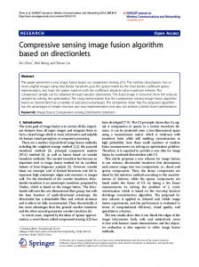
Figure 5: Top left: visual image, iconic. Top right: far infrared image. Middle left: fused image, standard fusion rule (selection). Middle right: fused image, iconic fusion rule (selection). Bottom left: Burt & Kolczynski fusion rule. Bottom right: iconic fusion rule (smooth). Top (input) images by courtesy of Xenics.

per band and per location we determine the similarity of the detail coefficients of the input images in a small region surrounding the location. We put several requirements to the scheme to be, based on desired outcomes for local circumstances. For convenience we introduce σkI (.|p) = Sign(ckI (.|p))

and

σkA (.|p) = Sign(ckA (.|p))

(where Sign is the well-known sign function with values +1 for a positive argument, −1 for a negative argument and 0 for a zero argument). If signs are opposite, we demand that ωkA (.|p) = −δkA (.), provided that the absolute local match measure |mkIA (.|p)| ≈ 1. If the local match measure happens to be around 0 (orthogonality) we want to resort to the above standard scheme. Likewise, when signs are not opposite we also want to resort to the standard scheme. These

requirements lead to the following scheme ωkI (.|p) = δkI (.), ωkA (.|p) = δkA (.)( 1 − |mkIA (.|p)| (1 − σkI (.|p)σkA (.|p)) ).

(4)

Inserting (4) into (2) yields ckF (.|p) = δkI (.)ckI (.|p) + δkA (.)( (1 − |mkIA (.|p))ckA (.|p)+ |mkIA (.|p)|σkI (.|p)|ckA (.|p)|).

(5)

We refer to the above rule as the smooth iconic fusion rule. Alternatively, a selection (i.e. thresholded) variant of rule (4) leads to the following composite coefficient:  ckI (.|p) δkI (.) ≥ δkA (.)    ckA (.|p) δ kI (.) < δkA (.) & ckF (.|p) = mk (.|p) < T  IA   k k σI (.|p)|cA (.|p)| otherwise (6)

155


for a threshold T , e.g. T = 12 . In the case of three or more input images, one again just selects one image as the iconic one and the generalisation is straightforward.

4

MORE RESULTS

Figure 5 shows results for a real-life surveillance example (in particular do watch the poles). The result at the middle left is based on the standard fusion rule (selection), the result at the middle right is based on the iconic fusion rule (6) (selection). In this section, for comparison, we point to additional results for the smooth variant of the said iconic fusion (bottom right) and for the rule of Burt & Kolczynski (bottom left). The latter rule implies that where similarity is low ( mkIA (.|p) < T ) the maximum selection rule is applied, where similarity is high ( mkIA (.|p) ≥ T (1 − mkIA (.|p)) ) the rule is presented by ωkI (.) = 12 − 12 (1 − T ) and ωkA (.) = 1−ωkI (.) which comes close to averaging mode. An important difference with the iconic fusion rule is that the outcome is symmetric with respect to interchanging the input images. Contrary to the new iconic fusion rule which tries, roughly speaking, to convert the infrared contrasts into visual light contrasts and interchanging the input images then would imply converting visual light contrasts into infrared contrasts.

4.1

Fusion Metrics

Due to lack of a ground-truth, especially in the context of multimodality, quantitative assessment of fusion is quite a challenge, and still appears an open problem. Many different metrics have already been proposed, but they rate algorithms differently (Liu et al., 2012). A rather general metric as the mutual information fusion metric persistently favors fusion by simply averaging input images (Cvejic et al., 2006), and looks not very suited for our new method. The choice for a metric is driven by the requirements of the application (Liu et al., 2012). In future research we plan to apply the 12 metrics used by the latter, and possibly devise an additional one of our own making, to make an objective assessment of our new method.

5

CONCLUDING REMARKS

Within the context of multiresolution schemes a new fusion rule has been proposed, coined iconic fusion

156

rule, so as to deal with opposite contrast which might occur in a set of multimodal images. The rule is a biased one, with the bias towards the contrasts observed (if any) in an image with a favoured spectrum, the so-called iconic image. Qualitative evidence for the soundness of the rule has been given by means of a few examples. A survey with quantitative assessment of several testproblems and applying a variety of quality measures is part of future research. Given the intent of the new method, quite likely a new quality measure needs to be devised so as to deal with images with opposite contrast.

ACKNOWLEDGEMENTS The research leading to these results has received funding from the European Community’s Seventh Framework Programme (FP7-ENV-2009-1) under grant agreement no FP7-ENV-244088 ”FIRESENSE - Fire Detection and Management through a MultiSensor Network for the Protection of Cultural Heritage Areas from the Risk of Fire and Extreme Weather”. We gratefully used images that have been provided to us by Xenics (Leuven, Belgium).

REFERENCES Burt, P. and Adelson, E. (1983). The laplacian pyramid as a compact image code. IEEE Transactions on Communications, 31(4):532–540. Burt, P. J. and Kolczynski, R. J. (1993). Enhanced image capture through fusion. In Proceedings Fourth International Conference on Computer Vision, pages 173– 182, Los Alamitos, California. IEEE Computer Society Press. Cvejic, N., Canagarajah, C. N., and Bull, D. R. (2006). Image fusion metric based on mutual information and tsallis entropy. Electronic Letters, 42(11):626–627. De Zeeuw, P. M. (2005). A multigrid approach to image processing. In Kimmel, R., Sochen, N., and Weickert, J., editors, Scale Space and PDE Methods in Computer Vision, volume 3459 of Lecture Notes in Computer Science, pages 396–407. Springer-Verlag, Berlin Heidelberg. De Zeeuw, P. M. (2007). The multigrid image transform. In Tai, X.-C., Lie, K. A., Chan, T. F., and Osher, S., editors, Image Processing Based on Partial Differential Equations, Mathematics and Visualization, pages 309 – 324. Springer Berlin Heidelberg. De Zeeuw, P. M., Piella, G., and Heijmans, H. J. A. M. (2004). A matlab toolbox for image fusion (matifus). CWI Report PNA-E0424, Centrum Wiskunde & Informatica, Amsterdam.


Forster, B., van de Ville, D., Berent, J., Sage, D., and Unser, M. (2004). Complex wavelets for extended depth-offield: A new method for the fusion of multichannel microscopy images,. Microscopy Research and Technique, 65:33–42. Han, J., Pauwels, E., and de Zeeuw, P. (2011). Visible and infrared image registration employing line-based geometric analysis. MUSCLE International Workshop on Computational Intelligence for Multimedia Understanding, Pisa (Italy), Accepted for publication. Li, H., Manjunath, B. S., and Mitra, S. K. (1995). Multisensor image fusion using the wavelet transform. Graphical Models and Image Processing, 57(3):235–245. Liu, Z., Blasch, E., Xue, Z., Zhao, J., Laganière, R., and Wu, W. (2012). Objective assessment of multiresolution image fusion algorithms for context enhancement in night vision: a comparative study. IEEE Trans. on Pattern Analysis and Machine Intelligence, 34(1):94– 109. Mallat, S. (1989). A theory for multiresolution signal decomposition: the wavelet representation. IEEE Pattern Analysis and Machine Intelligence, 11(7):674– 693. Piella, G. (2003a). Adaptive Wavelets and their Applications to Image Fusion and Compression. PhD thesis, CWI & University of Amsterdam. Piella, G. (2003b). A general framework for multiresolution image fusion: from pixels to regions. Information Fusion, 9:259–280. Simoncelli, E. and Freeman, W. (1995). The steerable pyramid: a flexible architecture for multi-scale derivative computation. In Proceedings of the IEEE International Conference on Image Processing, pages 444— 447. IEEE Signal Processing Society. Zitová, B. and Flusser, J. (2003). Image registration methods: a survey. Image and Vision Computing, 21:977– 1000.

157