MULTIPHASE IMAGE SEGMENTATION AND ... - Semantic Scholar

Preprint, IFB-Report No. 13 (12/2007), Institute of Mathematics and Scientific Computing, University of Graz.

MULTIPHASE IMAGE SEGMENTATION AND MODULATION RECOVERY BASED ON SHAPE AND TOPOLOGICAL SENSITIVITY ¨ M. HINTERMULLER AND A. LAURAIN

Abstract. Topological sensitivity analysis is performed for the piecewise constant Mumford-Shah functional. Topological and shape derivatives are combined in order to derive an algorithm for image segmentation with fully automatized initialization. Segmentation of 2D and 3D data is presented. Further, a generalized Mumford-Shah functional is proposed and numerically investigated for the segmentation of images modulated due to, e.g., coil sensitivities.

Keywords. Image processing, k-means clustering, modulation recovery, Mumford-Shah functional, piecewise constant recontruction, segmentation, shape and topological sensitivity. 1. Introduction Mathematical image segmentation is concerned with the task of partitioning a given image into disjoint (homogeneous) regions [13]. Among the many available paradigms, the approach due to Mumford and Shah [14] turned out to be particularly useful, as it simultaneously denoises and segments the image. It consists in minimizing the functional Z Z 2 (1) Jν (u, Γ) = (f − u) + µ |∇u|2 + νH1 (Γ), Ω

Ω\Γ

where f : Ω 7−→ [0, 1] denotes given image data (intensity map) on the image domain Ω ⊂ Rd and H1 (·) is the one-dimensional Hausdorff-measure. The function u represents the reconstructed image and Γ denotes the reconstructed contours (edge set) of the image. The parameters µ and ν penalize deviations from homogeneity on the pieces and the length of the perimeter of the pieces, respectively. While the original approach due to Mumford and Shah admits some variation of the reconstructed image on the disjoint pieces, in [1, 21] Chan and Vese considered a limitation to piecewise constant functions (Chan-Vese model). In this case, the original Mumford-Shah problem reduces to Z (2) min Jν (u, Γ) = (f − u)2 + νH1 (Γ). u,Γ

Ω

Moreover, for given m ∈ N, u is defined as m X (3) u= ci χΩi , i=1

This research was supported by the Austrian Ministry of Science and Research and the Austrian Science Fund FWF under START-grant Y305 ”Interfaces and Free Boundaries”. The original publication is available at www.springerlink.com. 1

¨ M. HINTERMULLER AND A. LAURAIN

2

with ci ≥ 0 the ”gray-value” (or phase) on the segment Ωi . Here χΩi denotes the characteristic function of Ωi . Hence, for the minimization of Jν , besides the determination of ci , the optimal location of Ωi becomes an issue. The latter corresponds to finding a topological distribution of the Ωi in Ω. For this purpose, in [7] a discrete topological sensitivity technique is considered for solving the piecewise constant Mumford-Shah problem. In the present paper, we first introduce topological sensitivity analysis in the continuous setting (where the original Mumford-Shah problem is posed as well). Compared to earlier methods, this approach has several benefits such as an automatized initialization which ultimately result in a highly efficient (with respect to iteration counts and CPU-time consumption) algorithm for image segmentation; see also section 4.2 for a numerical comparison. In a second part of the paper (see section 5) we are interested in minimizing the following, more general version of (1): Z Z Z 2 p 2 (4) Jν (u, Γ, σ) = (f − σu) + δ |∇ σ| + µ |∇u|2 + νH1 (Γ), Ω

Ω

Ω\Γ

where σ, which is assumed to be unknown, models a potential modulation of the image due to, e.g., coil sensitivities during image acquisition; see figure 10 on page 30 for an example, where the image on the right in the first row is a modulated version of the one on the left. Typically, σ is a smooth function which we do assume to be independent of u. The term in (4) involving ∇p σ acts as a regularization of σ. The choice of p ≥ 1 regulates smoothness. Further we have 0 ≤ σ ≤ σ < ∞ a.e. in Ω. In the piecewise constant Mumford-Shah context we solve Z Z min Jν (u, Γ, σ) = (5) (f − σu)2 + δ |∇p σ|2 + νH1 (Γ). u,Γ,σ

Ω

Ω

This formulation opens up new possibilities, but also new challenges in Mumford-Shah based image segmentation. To the best of our knowledge, very little research has been devoted to this version of the functional. The rest of the paper is organized as follows. In sections 2-4 we start our investigations by considering problem (2). In fact, in section 2 we introduce the topological derivative to the Mumford-Shah functional in the piecewise constant setting and without the perimeter term. We further design a solution algorithm and study its convergence properties. In section 3 we consider shape sensitivity in order to also include the perimeter term. In section 4 we report on numerical results for our approach. Then, in section 5 the generalized Mumford-Shah functional (5) is considered. For its numerical treatment, we introduce a modified version which, among others, takes care of the pointwise constraints on σ. The paper ends by a report on numerical results for simultaneous modulation recovery and image segmentation. 2. Piecewise constant Mumford-Shah functional and its topological sensitivity Let Ω ⊂ R2 be a bounded image domain, and let f : Ω 7−→ [0, 1] be the intensity map associated with a gray-level image. Further, m > 1 is an integer corresponding to the desired number of phases. The different phases

MULTIPHASE IMAGE SEGMENTATION AND MODULATION RECOVERY

3

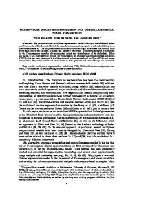
Figure 1. Partition of the domain Ω. are denoted by ci and the corresponding domains by Ωi , i ∈ {1, .., m}. Thus, we have the partitioning of Ω: Ω = ∪m i=1 Ωi ,

Ωi ∩ Ωj = ∅

∀i 6= j;

see figure 1. When minimizing Jν (u, Γ) with respect to u, we get for i = 1, .., m Z −1 ci = ci (Ωi ) = |Ωi | f (x) dx if Ωi 6= ∅ or ci = 0 otherwise. Ωi

Since f : Ω → [0, 1] we have ci ≥ 0 for all i. Let u be a bounded piecewise constant function defined by u(x) = ci

∀x ∈ Ωi ,

and denote by Γ the union of the boundaries Γi of the sets Ωi m Γ = ∪m i=1 Γi = ∪i=1 ∂Ωi .

(6)

Note that the sets Γi might have non-empty intersections. We can rewrite (2) in terms of Ωi only. For this purpose we introduce a new functional Jν : m Z m X νX 1 ν 2 (7) Jν ({Ωi }i∈{1,..,m} ) = (f (x) − ci ) dx + H (Γi ) + H1 (∂Ω). 2 2 Ωi i=1

1 2

i=1

ν 1 2 H (∂Ω)

The coefficient and the term in (7) come from the fact that each boundary Γi is counted twice in the sum (6). If we choose ν = 0 in (7), then we obtain m Z X (8) J0 ({Ωi }i∈{1,..,m} ) = J0 (u, Γ) = (f (x) − ci )2 dx. i=1

Ωi

2.1. Existence of an optimal solution. We show now that there exists a solution of the minimization problem for ν > 0 Minimize s.t. (9)

Jν ({Ωi }i∈{1,..,m} ) Ω = ∪m i=1 Ωi , Ωi ∩ Ωj = ∅ ∀i 6= j, Ωi measurable ∀i ∈ {1, .., m}.

¨ M. HINTERMULLER AND A. LAURAIN

4

Theorem 1. Problem (9) admits a solution {Ω∗i }i∈{1,..,m} . (n)

Proof. Let {Ωi }i∈{1,..,m} be a minimizing sequence for problem (9). Then (n)

we have for ν > 0 that H1 (Γi ) < M1 where M1 is a constant which does not depend on i or n. Since Ω is bounded, we have (n)

(n)

|Ωi | + H1 (Γi ) < M2 , for some constant M2 > 0. Thus, [8, Thm 2.3.10 (p. 61)] (see also [2, Thm 5.3 (p. 128)] and [24]) yields the existence of {Ω∗i }i∈{1,..,m} such that for all i ∈ {1, .., m}, χΩ(n) −→ χΩ∗i in L1 (Ω)

(10)

i

up to a subsequence. We immediately infer that (n)

|Ω∗i | = lim |Ωi |. n→∞

From (10) we get

Z

Z

Ω

f χΩ(n) → i

Ω

f χΩ∗i ,

and as a consequence (n)

ci Thus, we infer m Z X i=1

−→ c∗i .

(n)

(n) Ωi

(f (x) − ci )2 dx −→

m Z X i=1

Ω∗i

(f (x) − c∗i )2 dx.

From [8, Prop 2.3.6 (p. 60)] (see also [2, 24]) we also have (n)

H1 (Γ∗i ) ≤ lim inf H1 (Γi ). Gathering the previous results we obtain (n)

Jν ({Ω∗i }i∈{1,..,m} ) ≤ lim inf Jν ({Ωi }i∈{1,..,m} ) = min Jν ({Ωi }i∈{1,..,m} ), and hence

Jν ({Ω∗i }i∈{1,..,m} ) = min Jν ({Ωi }i∈{1,..,m} ). This proves the assertion.

¥

2.2. Topological derivative. In this section we set ν = 0 and write J instead of J0 . This is motivated by the fact that the perimeter term corresponds to lower dimensional sets. Keeping this term would induce a singularity in the topological asymptotic analysis. Rather it is dealt with by shape sensitivity in a subsequent section. We note that our treatment of the perimeter term follows a standard procedure in shape optimization. Let ρ > 0 be a positive scalar and let x0 be a point in Ωi . Then Bρ := B(x0 , ρ) denotes the ball of radius ρ and center x0 . The topological derivative Ti,j of J at x0 is defined in the following way: J (Ω1 , ..., Ωi \ Bρ , ..., Ωj ∪ Bρ , ..., Ωm ) (11)

= J ({Ωi }i∈{1,..,m} ) + πρ2 Ti,j (x0 ) + o(ρ2 );

see [19] for a definition in a more general shape and topology optimization context. It provides a criterion for removing a small part from Ωi and adding

MULTIPHASE IMAGE SEGMENTATION AND MODULATION RECOVERY

5

it to Ωj . In fact, if Ti,j (x0 ) is negative, then the functional J is decreasing for ρ sufficiently small. Therefore we define a matrix-valued function T containing the different topological derivatives corresponding to all possible cases: (12)

T := {Ti,j }(i,j)∈{1,..,m}2 .

From definition (11) we see that Ti,i ≡ 0 for all i ∈ {1, .., m}. Next we calculate the topological derivative Ti,j for i 6= j. Assuming |Ωi | > 0, we first compute the expansion of ci in the case where we ”remove material” from Ωi : Z Z 1 1 ci (Ωi \ Bρ ) − ci (Ωi ) = f (x) dx − f (x) dx |Ωi \ Bρ | Ωi \Bρ |Ωi | Ωi ! à Z |Bρ | 1 f (x) dx = ci (Ωi ) − |Ωi | |Bρ | Bρ à ! Z |Bρ |2 1 + ci (Ωi ) − f (x) dx . |Ωi | |Ωi \ Bρ | |Bρ | Bρ The expansion of cj when we ”add material” to Ωj depends on whether |Ωj | = 0 or not. If |Ωj | 6= 0, then we write à ! Z |Bρ | 1 cj (Ωj ∪ Bρ ) − cj (Ωj ) = − cj (Ωj ) − f (x) dx |Ωj | |Bρ | Bρ à ! Z |Bρ |2 1 cj (Ωj ) − + f (x) dx , |Ωj | |Ωj ∪ Bρ | |Bρ | Bρ otherwise, if |Ωj | = 0, we have

Z −1

cj (Ωj ∪ Bρ ) = |Bρ |

f (x) dx. Bρ

Now, if |Ωj | = 6 0, then we obtain J (Ω1 ,..., Ωi \ Bρ , ..., Ωj ∪ Bρ , ..., Ωm ) − J ({Ωi }i∈{1,..,m} ) Z Z 2 = (f (x) − cj (Ωj ∪ Bρ )) dx + (f (x) − ci (Ωi \ Bρ ))2 dx Ωj ∪Bρ

Z

Ωi \Bρ

Z

− Ωj

(f (x) − cj (Ωj ))2 dx −

Ωi

(f (x) − ci (Ωi ))2 dx.

Taking into account the expansions of ci (Ωi \ Bρ ) and cj (Ωj ∪ Bρ ) results in J (Ω1 ,..., Ωi \ Bρ , ..., Ωj ∪ Bρ , ..., Ωm ) − J ({Ωi }i∈{1,..,m} ) Z = (f (x) − cj (Ωj ))2 − (f (x) − ci (Ωi ))2 dx Bρ

|Bρ | +2 |Ωj |

Ã

1 cj (Ωj ) − |Bρ |

Z

!Z f (x) dx

Bρ

Ωj

(f (x) − cj (Ωj )) dx

¨ M. HINTERMULLER AND A. LAURAIN

6

|Bρ | −2 |Ωi |

Ã

1 ci (Ωi ) − |Bρ |

!Z

Z

f (x) dx Ωi

Bρ

(f (x) − ci (Ωi )) dx + O(|Bρ |)

as R |Bρ | → 0 for ρ → 0.R From Lebesgue’s differentiation theorem [3] and Ωi (f (x) − ci (Ωi )) dx = Ωj (f (x) − cj (Ωj )) dx = 0 we infer (13) Ti,j (x0 ) = (f (x0 ) − cj (Ωj ))2 − (f (x0 ) − ci (Ωi ))2 for almost all x0 ∈ Ω. In the case where |Ωj | = 0 we have J (Ω1 ,..., Ωi \ Bρ , ..., Ωj ∪ Bρ , ..., Ωm ) − J ({Ωi }i∈{1,..,m} ) Z Z = (f (x) − cj (Ωj ∪ Bρ ))2 dx + (f (x) − ci (Ωi \ Bρ ))2 dx Bρ Ωi \Bρ Z − (f (x) − ci (Ωi ))2 dx Ωi Z = (f (x) − cj (Ωj ∪ Bρ ))2 − (f (x) − ci (Ωi ))2 dx Bρ

|Bρ | −2 |Ωi |

Ã

1 ci (Ωi ) − |Bρ |

Z

!Z f (x) dx

Bρ

Ωi

(f (x) − ci (Ωi )) dx

+ O(|Bρ |) as |Bρ | → 0 for ρ → 0. Since cj (Ωj ∪ Bρ ) = |Bρ |−1 almost all x0 ∈ Ω, we get (14)

R Bρ

f (x) dx → f (x0 ) for

Ti,j (x0 ) = −(f (x0 ) − ci (Ωi ))2 for almost all x0 ∈ Ω.

2.3. Algorithm for topological derivative. The initialization of our algorithmic procedure for solving (9) with ν = 0 uses Ω1 = Ω and Ωi = ∅ for all i > 1. Then we determine Ω2 by computing T1,2 . Following equation (11), we may choose Ω2 = {x0 ∈ Ω1 | T1,2 (x0 ) < 0} . Actually, since the topological derivative is only a local criterion, we prefer to change the domain Ω1 only when the topological derivative is sufficiently negative. In order to do that, we fix a prescribed tolerance 0 ≤ γ < 1 and set ½ ¾ Ω2 =

x0 ∈ Ω1 | T1,2 (x0 ) < γ min T1,2 (y) . y∈Ω1

Once we have initialized the sets Ωk , k = 1, .., i < m, we set ¾ i ½ [ (15) Ωi+1 = x0 ∈ Ωk | Tk,i+1 (x0 ) < γ min Tk,i+1 (y) . k=1

y∈Ωk

Therefore the topological algorithm operates in two steps. In the first step we initialize all the domains Ωi , and in the second step we modify the domains according to the topological derivatives between all the m existing domains. Ideally, convergence is reached when all the topological derivatives are zero.

MULTIPHASE IMAGE SEGMENTATION AND MODULATION RECOVERY

7

However, for numerical purposes, we stop the algorithm as soon as   m m X X (l) (0) kTi,j k2 ≤ µt 1 + kTi,j k2  , i,j=1 (l)

i,j=1 (l)

where kTi,j k2 is the L2 -norm of Ti,j and 0 < µt ¿ 1 denotes a user-specified stopping tolerance. In what follows we propose two different algorithms. The first algorithm is based on the previous idea, which is a standard technique for using the topological derivative. The second one turns out to be much faster in practice. Below, theorem 2 provides a relation between the two methods.

¨ M. HINTERMULLER AND A. LAURAIN

8

Algorithm 1: Initialization Input: Ω, f , m, γ, µt Output: Ωi , ci , i = 1, .., m. R (0) (0) Initialization: Set Ω1 := Ω and, thus, c1 = |Ω|−1 Ω f (x) dx. Set l := 0. for i = 1, .., m − 1 do for k = 1, .., i do R (0) (0) Compute ck = |Ωk |−1 Ω(0) f (x) dx. k

(0)

(0)

Compute Tk,i+1 (x0 ) = −(f (x0 ) − ck )2 . (0)

(0)

Initialize Ωi+1 by using (15), and update Ωk by setting ( (0)

(0)

(0)

Ωk = Ωk \ end end while

(0)

) (0)

x0 ∈ Ωk | Tk,i+1 (x0 ) < γ min Tk,i+1 (y) . (0) y∈Ωk

´ ³ Pm (0) (l) kT k kT k > µ 1 + t i,j=1 i,j=1 i,j 2 do i,j 2

Pm

(l+1)

(l)

Set Ωk = Ωk ∀k ∈ {1, .., m}. for i = 1, .., m do (l+1) (l) Compute Ti,j for all x0 ∈ Ωi and all j ∈ {1, .., m}. Define (l+1)

Ti Determine the sets (l+1) Ai (l+1)

Ωi

(x0 ) =

min

j∈{1,..,m}

(l+1)

Ti,j

(x0 ).

(

=

) x0 ∈

(l) Ωi

(l+1)

\ Ai

= Ωi

|

(l+1) Ti (x0 )

(l+1)

0 and |Ωi ∆Ωi | > 0 ∀i) or l = 0] do (l)

(l)

(l)

Compute di n , i ∈ {2, .., m}, set d1 < 0, odm+1 = max(f ). (l+1) (l) (l) Set Ωi = x ∈ Ω | di < f (x) ≤ di+1 ∀i ∈ {1, .., m}. for i = 1, .., m do (l+1) if |Ωi | > 0 then (l+1) (l+1) −1 R Update ci = |Ωi | (l+1) f (x) dx. Ω i

else (l+1) (l) (l) Choose arbitrary ci outside the interval [di−1 , di ]. end end set l = l + 1 end A few words on the algorithm are in order. First note that algorithm 2 for minimizing the piecewise constant Mumford-Shah functional (Chan-Vese model) without perimeter term is closely related to the k-means clustering algorithm; see, e.g., [5, 6, 11] for details on the latter. Secondly, in the else(l+1) (l) (l) branch of the if-statement alternative choices of ci even within [di−1 , di ] are possible. Keeping the same value than in the previous step , however, is only meaningful if at least one of the other ci -values changes. Our suggestion (l) (l) (l) in the else-branch above is motivated by the fact that ci ∈ [di−1 , di ] produced Ωl+1 = ∅. Further, below we show that algorithm 2 is similar to i algorithm 1 for γ = 0. We also prove a monotonicity property of algorithm

¨ M. HINTERMULLER AND A. LAURAIN

10

2; see Proposition 1 below. For the initialization of the phases one may use (max(f ) − min(f )) m+1 for instance, but other choices are possible. (0)

ci

= min(f ) + i

for i = 1, ..., m,

We start our investigation by proving several auxiliary results. In what follows, we assume (17)

(0)

(0)

min(f ) ≤ c1 < .. < ci

< .. < c(0) m ≤ max(f ).

Lemma 1. Define (18)

Ti,j (x) := (f (x) − cj )2 − (f (x) − ci )2

∀i, j ∈ {1, .., m},

∀x ∈ Ω.

Then Ti,j (x) = Ti,k (x) + Tk,j (x). Proof: The proof follows immediately from the definition of Ti,j .

¥

Note that Ti,j in (18) is an extended version of the topological derivative in (11) as x is arbitrary in Ω (and not just Ωi ). Lemma 2. Let Ti,j be defined as in (18). Then ½ either ci < cj and Ti,j (x) < 0 ⇐⇒ or ci > cj and

f (x) > f (x)
dp+1 . Then, according to lemma 2, we get Tp,p+1 (x) < 0, and, according to lemma 1, Tk,p (x) + Tp,p+1 (x) = Tk,p+1 (x) < Tk,p (x). This, however, contradicts our assumption (19). Thus f (x) ≤ dp+1 .

MULTIPHASE IMAGE SEGMENTATION AND MODULATION RECOVERY

11

Now we study the second inequality. If p = 1, the inequality is fulfilled since d1 < 0 and f (x) ≥ 0. Now assume that f (x) ≤ dp and p > 1. First, if f (x) < dp , we get Tp,p−1 (x) < 0 and Tk,p (x) + Tp,p−1 (x) = Tk,p−1 (x) < Tk,p (x), which is impossible due to our assumption (19). Thus, we have f (x) ≥ dp . Further, if f (x) = dp , it is easy to see that Tp,p−1 (x) = 0. Hence we have Tk,p (x) + Tp,p−1 (x) = Tk,p−1 (x) = Tk,p (x) =

min

l∈{1,..,m}

Tk,l (x).

Again, this contradicts (19). Therefore, f (x) > dp holds true. Conversely, assume that f (x) satisfies (20) for some 1 < pˆ < m, and let q ≥ pˆ + 1. Then cpˆ + cq f (x) ≤ dpˆ+1 ≤ , 2 and, according to lemma 2, we get Tq,ˆp (x) ≤ 0 and, thus, Tpˆ,q (x) ≥ 0. Further Tk,ˆp (x) + Tpˆ,q (x) = Tk,q (x) ≥ Tk,ˆp (x). In a similar way, if q ≤ pˆ − 1, we have cpˆ + cq , 2 and, according to lemma 2, we get Tq,ˆp (x) ≤ 0 and, thus, Tpˆ,q (x) ≥ 0. Further Tk,ˆp (x) + Tpˆ,q (x) = Tk,q (x) > Tk,ˆp (x). f (x) > dpˆ ≥

Finally we get Tk,ˆp (x) =

min

l∈{1,..,m}

Tk,l (x),

which proves the converse statement.

¥

Now we are going to prove a theorem which shows that algorithm 2 and algorithm 1 have a similar behavior. (l)

Theorem 2. Let l ≥ 1. Assume that Ωi , i ∈ {1, .., m}, and the corre(l) (l) (l) sponding min(f ) ≤ c1 < .. < ci < .. < cm ≤ max(f ) are given. Assume that ˆlk (x) = argmin (21) Tk,l (x) l∈{1,..,m}

is unique for all x in Ω and k ∈ {1, .., m}. Then, after one iteration of the main loop of algorithm 1 with γ = 0, we get: ³n o (l+1) (l) (l) Ωk = x ∈ Ω | dk < f (x) ≤ dk+1 n o´ n o (l) (l) (l) (l) ∪ x ∈ Ωk | f (x) = dk \ x ∈ Ωk+1 | f (x) = dk+1 . (l+1)

Proof: In algorithm 1, Ak ( (l+1)

Ak

=

(l)

is defined in the following way: ) (l+1)

x ∈ Ωk | Tk

(l+1)

(x) < γ min Tk (l) y∈Ωi

(y) .

¨ M. HINTERMULLER AND A. LAURAIN

12

If γ = 0 we have (l+1)

Ak

n o (l) (l+1) = x ∈ Ωk | T k (x) < 0 .

which can be written as (l+1) Ak

(22)

=

m [

(l+1)

Bj,k ,

j=1

with (l+1)

Bj,k

n o (l) (l) (l) (l+1) = x ∈ Ωk | dj < f (x) ≤ dj+1 and Tk (x) < 0 .

Now we analyse different cases for Bj,k : (l+1)

First case: If k = j, then Bj,k get from lemma 3

(l+1)

0 = Tk,k (l+1)

and, thus, Tk

(l)

(l)

= ∅. Indeed, if dk < f (x) ≤ dk+1 , then we

(x) =

(l+1)

min

l∈{1,..,m}

Tk,l

(x)

(x) = 0.

Second case: If k > j + 1, then n o (l+1) (l) (l) (l) Bj,k = x ∈ Ωk | dj < f (x) ≤ dj+1 . Indeed, we have (l)

f (x) ≤ (l+1)

Thus, Tk,j

(l) dj+1

=

(l)

(l)

cj + cj+1 2


(l+1) Tk,j (x)

(l) dj

=

(l)

(l)

cj−1 + cj 2

≥

(l)

ck + cj 2

(l+1)

which implies < 0 according to lemma 2. Thus Tk Finally, in this case we get n o (l+1) (l) (l) (l) Bj,k = x ∈ Ωk | dj < f (x) ≤ dj+1 .

(x) < 0.

MULTIPHASE IMAGE SEGMENTATION AND MODULATION RECOVERY

13

In view of algorithm 1 and assumption (21), after one iteration, we obtain   m n o [ (l+1) (l) (l+1) (l+1) (l+1) (l+1) Ωk = (Ωk \ Ak ) ∪  x ∈ Ai | Ti,k (x) = Ti (x)  i=1,i6=k

 (l)

(l+1)

= (Ωk \ Ak

m [

)∪





 m n o [ (l) (l+1) (l+1) (l+1)  ∩ x ∈ Ωi | Ti,k (x) = Ti (x)  Ai i=1,i6=k

i=1,i6=k

Now according to (22) and in view of lemma 3 we have     m m m n o [ [ [ (l+1) (l) (l+1) (l+1) (l) (l+1) (l+1) Ωk = (Ωk \ Ak ) ∪  Bj,i  ∩  x ∈ Ωi | Ti,k (x) = Ti (x)  i=1,i6=k j=1

 (l)

(l+1)

= (Ωk \ Ak

)∪

m [

i=1,i6=k

 m ³ n o´ [ (l+1) (l) (l) (l) Bj,i ∩ x ∈ Ωi | dk < f (x) ≤ dk+1  .

j=1 i=1,i6=k (l+1)

According to our above characterization of Bj,k we get n o (l+1) (l) (l) (l) Bj,i ∩ x ∈ Ωi | dk < f (x) ≤ dk+1 = ∅ if j 6= k. As a consequence  (l+1)

Ωk

(l)

(l+1)

= (Ωk \ Ak

)∪

m [

 n o (l) (l) (l) x ∈ Ωi | dk < f (x) ≤ dk+1 

i=1,i6=k,k+1

n o (l) (l) (l) ∪ x ∈ Ωk+1 | dk < f (x) < dk+1 . In addition we have (l)

(l+1)

Ωk \ Ak

n o (l) (l+1) x ∈ Ωk | Tk (x) ≥ 0 n o (l) (l) (l) = x ∈ Ωk | dk ≤ f (x) ≤ dk+1

=

which leads to n o n o (l+1) (l) (l) (l) (l) (l) (l) Ωk = x ∈ Ωk | dk ≤ f (x) ≤ dk+1 ∪ x ∈ Ωk+1 | dk < f (x) < dk+1   m n o [ (l) (l) (l) ∪ x ∈ Ωi | dk < f (x) ≤ dk+1  , i=1,i6=k,k+1

and finally (l+1)

Ωk

=

³n o (l) (l) x ∈ Ω | dk < f (x) ≤ dk+1 n o´ n o (l) (l) (l) (l) ∪ x ∈ Ωk | f (x) = dk \ x ∈ Ωk+1 | f (x) = dk+1 .

This concludes the proof.

¥

14

¨ M. HINTERMULLER AND A. LAURAIN (l+1)

Remark 1. Theorem 2 states that the updated domain Ωk of algorithm (l+1) 1 differs from the updated domain Ωk of algorithm 2 by the set n o n o (l) (l) (l) (l) x ∈ Ωk | f (x) = dk \ x ∈ Ωk+1 | f (x) = dk+1 , which will be negligible for most ”real-life” images. Moreover, whenever the index ˆlk (x) in (21) is not unique, x may be moved into any of the sets yielding the minimum. In our implementation the set with the smallest index is chosen. In practice such a non-uniqueness typically occurs only for a few pixels during the segmentation except maybe in certain cases of piecewise constant data. Next, we establish a monotonicity result for Algorithm 2. For its proof we need the following auxiliary result, which requires the mean value f¯D of a given function f : A → R, where A is nonempty and bounded and D ⊂ A with positive Lebesgue measure |D|, defined by Z −1 ¯ fD = |D| f (x) dx. D

Lemma 4. Let f ∈ L∞ (A, R), A ⊂ RN bounded, N ≥ 1, and define A1 = {x ∈ A | a < f (x) ≤ b}, A2 = {x ∈ A | c < f (x) ≤ d} with a ≤ c and b ≤ d. We assume that |A1 | 6= 0 and |A2 | = 6 0. Then we have f¯A1 ≤ f¯A2 . Proof: First of all, if c ≥ b we immediately find f¯A > c ≥ b ≥ f¯A . 2

1

On the other hand, if c < b we define the sets B1 = {x ∈ A | c < f (x) ≤ b}, C1 = {x ∈ A | a < f (x) ≤ c}. Note that |B1 | = 0 and |C1 | = 0 cannot happen simultaneously since A1 = B1 ∪ C1 and |A1 | = 6 0. If |B1 | = 0, then we have f¯A > c ≥ f¯A . 2

1

Therefore, in what follows, we assume that |B1 | 6= 0. If |C1 | = 0, then A1 = B1 and, consequently, f¯A = f¯B ; 1

1

otherwise, if |C1 | 6= 0, then there holds (23) f¯A1 < f¯B1 . Indeed, first note that f¯C1 < f¯B1 and further µZ Z −1 ¯ ¯ fA1 − fB1 = |A1 | f (x) dx + B1

=

C1

|B1 | ¯ |C1 | ¯ fB1 + fC − f¯B1 |A1 | |A1 | 1

¶ f (x) dx − f¯B1

MULTIPHASE IMAGE SEGMENTATION AND MODULATION RECOVERY

15

|B1 | ¯ |C1 | ¯ fB1 + fB − f¯B1 |A1 | |A1 | 1 < f¯B1 − f¯B1 < 0.
n0 , then we can write for all k ∈ {1, .., m − 1}: (n+1)

ck and hence

(n+1)

+ ck+1 2

(n+1)

(n)

(n)

c + ck+1 ≥ k 2 (n)

dk+1 ≥ dk+1 . Since (n+1)

Ωk and

(n+2)

Ωk

n o (n) (n) = x ∈ Ω | dk < f (x) ≤ dk+1

∀k ∈ {1, .., m}

n o (n+1) (n+1) = x ∈ Ω | dk < f (x) ≤ dk+1 (n+1)

∀k ∈ {1, .., m}

(n+2)

we apply lemma 4 with A1 = Ωk and A2 = Ωk and get (n+2) (n+1) ck ≥ ck .

for k ∈ {2, .., m − 1}

¨ M. HINTERMULLER AND A. LAURAIN

16

For k = 1 and k = m we obtain a similar result. Concerning the second part of the proposition, we note that if we assume that (25) is true for some n ≥ n1 , then we can write for all k ∈ {1, .., m − 1}: (n+1)

c c∗k + c∗k+1 ≥ k 2 and further

(n+1)

+ ck+1 2

(n+1)

d∗k+1 ≥ dk+1 . Since

© ª Ω∗k = x ∈ Ω | d∗k < f (x) ≤ d∗k+1

and (n+2)

Ωk

∀k ∈ {1, .., m}

n o (n+1) (n+1) = x ∈ Ω | dk < f (x) ≤ dk+1 (n+2)

we apply lemma 4 with A1 = Ωk get

and A2 = Ω∗k for k ∈ {2, .., m − 1} and

(n+2)

ck

∀k ∈ {1, .., m}

≤ c∗k .

For k = 1 and k = m we obtain a similar result. ¥ In our numerical experience the prerequisits of Proposition 1 are typically met after a few iterations. In fact, we find an iteration n ¯ such that all ck values increase (compared to their respective value in the previous iteration). (n) In such a situation Proposition 1 guarantees that the sequences {ck }, k = (¯ n) 1, . . . , m, are monotonically increasing for n ≥ n ¯ . In addition, if ck ≤ c∗k (n) for all k = 1, . . . , m then ck , k = 1, . . . , m , approaches the optimal value from below as stated in the second part of the proposition. 3. Shape derivatives of the Mumford-Shah functional and the level set framework Next we recall some theoretical aspects of shape optimization; see [20]. The analysis here is greatly simplified by the fact that we do not deal with partial differential equations. Let Γ be defined as in (6) and let ni be the outward unit normal vector to Ωi . In what follows V (t, x) is a smooth vector field defined on [0, T ] × Ω with V (t, x) · ni (x) = 0 for almost every x ∈ ∂Ω all t ∈ [0, T ] and all i ∈ {1, .., m}. If the unit exterior normal vector ni is not defined at a singular x ∈ Γ we assume that V (t, x) = 0. The vector field V is said to be admissible if it satisfies these conditions. Let x = x(t, x) denote the solution of the initial value problem (26) (27)

d x(t, x) = V (t, x(t, x)), dt x(0, x) = x.

with x ∈ Ω and t ∈ [0, T ], and we denote by T t : Ω → Ω the time-t map with respect to (26)-(27), i.e. T t (x) = x(t, x). We set Γt = T t (Γ). The Eulerian semi-derivative of J at Γ in direction of the vector field V is defined as the limit 1 dJ(Γ; V ) = lim (J(Γt ) − J(Γ)), t→0 t

MULTIPHASE IMAGE SEGMENTATION AND MODULATION RECOVERY

17

if it exists. A classical result on the structure of the shape derivative for smooth domains states (see [20]) that there exists a distribution ∇J on Γ such that dJ(Γ; V ) = h∇J, vn iΓ , where vn (x) = V (0, x) · n(x) and h·, ·iΓ denotes an appropriate duality pairing. If this duality pairing can be realized as an integral over Γ we have Z (28) dJ(Γ; V ) = ∇Jvn dΓ, Γ

and we are able to use a gradient method by choosing vn = −∇J; otherwise some presmoothing is necessary. In the level set framework [15, 16, 18], the two-dimensional domain Ωi is represented as the set of points where a three dimensional function φ defined over Ω is negative. It is also assumed that φ(Ω \ Ωi ) > 0 with φ Lipschitz continuous. Since we have not only one but a collection of domains Ωi , i ∈ {1, .., m}, it is straightforward to see that k level set functions allow for 2k domains. Therefore k can be chosen as the closest integer value greater than or equal to lnlnm 2 . For instance, with m = 4 we get k = 2. For the sake of simplicity, we restrict ourselves to the two-dimensional case and m = 4 in what follows. Therefore, we define two level sets functions φ1 and φ2 and the sets D1 and D2 such that (29) (30)

D1 := Ω1 ∪ Ω2 = {x ∈ Ω | φ1 (x) < 0} , D2 := Ω1 ∪ Ω3 = {x ∈ Ω | φ2 (x) < 0} .

Then, for instance, the set Ω1 can be deduced by Ω1 = {x ∈ Ω | φ1 (x) < 0 and φ2 (x) < 0} . There exists a simple relation between the evolution of a level set function φ and the vector field V (t, x), which corresponds to the moving boundary Γt . Actually, the level set function φ is the solution of the Hamilton-Jacobi equation (31) (32)

φt (t, x) + vnext (t, x)|∇φ(t, x)| = 0 for φ(0, x) = φ0 (x)

(t, x) ∈ [0, T ] × Ω, for x ∈ Ω

where φt stands for the time derivative of φ and φ0 is given initial data. For example, φ0 may correspond to the signed distance function of the initial contour Γ0 . Note that vn is defined only on Γ, therefore it is necessary to define an extension vnext to the entire domain. This extension is used in (31). There are several ways to achieve such an extension; see, for instance, [9]. 3.1. Shape sensitivity analysis. Now we return to our initial multiphase formulation (2). For convenience, we use the notation Jν (Γ) = Jν ({Ωi }i∈[1,m] ). Using the calculus developed in [20] and assuming that Γi ∩ Γj , i 6= j, is sufficiently smooth, the shape derivative of Jν (Γ) in the direction of the vector field V is given by Z m X 2 (f (x) − ci )c0i (Γ; V ) dx dJν (Γ; V ) = i=1

Ωi

¨ M. HINTERMULLER AND A. LAURAIN

18

Figure 2. Partition of Ω and level set functions φ1 and φ2 .

+

ÃZ m X m X i=1 j6=i

¢ ¡ ν (f (x) − ci )2 + κi (x) vni (x) dx, 2 Γi ∩Γj

! ,

where Γi := ∂Ωi and κi is the curvature of Γi , ni is the outer unit normal vector to Ωi , and c0i (Γ; V ) denotes the shape derivative of ci at Γ in the direction V . Actually, since c0i (Γ; V ) is a scalar, we have Z m m Z X X 0 0 (f (x) − ci ) dx = 0, (f (x) − ci )ci (Γ; V ) dx = ci (Γ; V ) i=1

Ωi

i=1

Ωi

as ci is the mean value of f over the domain Ωi . Thus, we obtain (33) m m Z ¡ ¢ 1 XX (f (x) − ci )2 − (f (x) − cj )2 + νκi (x) vni (x) dx. dJν (Γ; V ) = 2 Γi ∩Γj i=1 j6=i

Therefore, we identify the shape gradient as in (28) by ν ∇Jν (x) = (f (x) − ci )2 − (f (x) − cj )2 + κi (x) a.e. on Γi ∩ Γj 2 for i, j = 1, . . . m with j 6= i. Extending this expression to Γi , i = 1, . . . , m, we define the steepest descent flow by ν (34) vni (x) = −(f (x) − ci )2 + (f (x) − cj )2 − κi (x) a.e. on Γi ; 2 see [1] for a related expression. The normal velocity field in (34) is defined on Γi , but for the purpose of solving the Hamilton-Jacobi equation, we need to define it on the boundaries of D1 and D2 . We must take into account the fact that the intersections of the Γi , i ∈ {1, .., m}, are non-empty. From the definition of D1 we get ∂D1 \ ∂Ω = (Γ1 ∪ Γ2 ) ∩ (Γ3 ∪ Γ4 ) = (Γ1 ∩ Γ3 ) ∪ (Γ1 ∩ Γ4 ) ∪ (Γ2 ∩ Γ3 ) ∪ (Γ2 ∩ Γ4 ). From (34), and in view of κi = −κj on Γi ∩ Γj for i, j ∈ {1, .., m}, we deduce the values of the velocity fields on the boundaries of D1 and D2 , respectively, as (35)

vnD1

= −(f − c12 )2 + (f − c34 )2 − νκD1 a.e. on ∂D1 ,

(36)

vnD2

= −(f − c13 )2 + (f − c24 )2 − νκD2 a.e. on ∂D2 ,

MULTIPHASE IMAGE SEGMENTATION AND MODULATION RECOVERY

19

where cij designates the piecewise constant function cij (x) = ci if x ∈ Γi , cij (x) = cj if x ∈ Γj , and κD1 , κD2 are the curvatures of D1 and D2 , respectively. 3.2. Algorithm for shape derivative. The starting point of our shape optimization algorithm is the numerical solution obtained after running algorithm 2. In what follows, the superscript (l) refers to the l-th iterate of the discrete counterpart of the respective continuous variable. In a similar way as for the algorithm for topological derivative we stop the algorithm as soon as (l)

(l)

(0)

(0)

max(kV1 k2 , kV2 k2 ) ≤ µ1s (1 + max(kV1 k2 , kV2 k2 )), or |Jν (Γ(l+1) ) − Jν (Γ(l) )| ≤ µ2s (1 + Jν (Γ(0) )) where 0 < µ1s , µ2s ¿ 1 are user-specified stopping tolerances. (0)

(0)

step 1 Initialize by choosing φ1 and φ2 as the signed distance (0) (0) (0) (0) functions to Ω1 ∪ Ω2 and Ω1 ∪ Ω3 , respectively, so that (0) (29)-(30) is satisfied. Here, the sets Ωi , i ∈ {1, .., m}, come from Algorithm 1; set l = 0. (l) (l) (l) (l) step 2 Compute the normal velocities vn,1 and vn,2 for φ1 and φ2 (l)

(l)

according to (35)-(36). If kvn,1 k = 0 and kvn,2 k = 0, then stop; otherwise continue with step 3. (l) (l) step 3 Extend the normal velocity vn,1 and vn,2 to the whole domain (l)

Ω as described in (57), and update the level set functions φ1 (l) and φ2 by solving the Hamilton-Jacobi equation (31). (l) step 4 Update the domains Ωi , i ∈ {1, .., m} according to (29)-(30) and put l = l + 1. Go to step 2. As before, in our numerical realization of the above scheme we replace k · k2 and µjs , j = 1, 2, by a discrete L2 -norm and µjs h, respectively. A line search procedure is performed to modify the time step in the discrete Hamilton-Jacobi equation; see (51). This is done by multiplying the time step by α > 0, which is determined such that a Armijo-type descent criterion is satisfied. In the iterative procedure below, one chooses some initial α0 > 0 and reduces this value by multiplying by β ∈ (0, 1), if necessary. For the description of the lines search, let λ > 0 be a given parameter and 0 < αs ¿ 1 denote a lower bound on α. Then the line search procedure of iteration l is as follows: (l)

(l)

step 1 If Jν (Γ(l+1) ) − Jν (Γ(l) ) ≤ −λα max(kV1 k2 , kV2 k2 ) then stop the line search and set α = min(2α, α0 ); else go to step 2. step 2 Set α := βα. If α < αs then stop the algorithm. step 3 Compute the new boundary Γ(l+1) . step 4 Compute the new value Jν (Γ(l+1) ). Go to step 1.

20

¨ M. HINTERMULLER AND A. LAURAIN

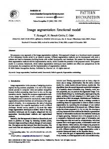
Finally we mention that in our numerics we use a narrow-band version of our level-set based shape optimization algorithm. 4. Numerics Now, we present different segmentation results. For topological sensitivity all results were obtained by algorithm 2. The number m of levels is fixed to m = 4 in all of our examples. The domain Ω is a square containing n2 pixels. For each example, the number of pixels and iterations, respectively, and the CPU-time in seconds are presented. In the line search procedure discussed above we use the parameter values β = 0.5 and λ = 10−2 . In our tests, the initial step size α0 is chosen as α0 = 10−4 . The constants for the stopping criteria described in the algorithms are chosen as µ1s = 5.102 , µ2s = 10, αs = 10−8 . The regularization parameter for the length of the contour is ν = 200 in all examples. All computations were performed on a standard desktop PC (Intel 3.20 GHz CPU with 2GB of RAM). 4.1. Numerical results. Example 1. The first example is an image of a plane; see figure 3. The topology optimization is extremely fast. It produces an excellent segmentation, but the boundaries of the Ωi ’s still require the application of the shape sensitivity step in order to account for the perimeter term in the Mumford-Shah functional. We point out that the shape optimization step usually is slower than the topology optimization phase. This is due to the additional work in the time-stepping of the Hamilton-Jacobi equation for advancing φ and the redistancing; see Table 1. Table 1 n2 Iterations topo Time topo Iterations shape Time shape 3902 11 0.11s 6 11.28s Example 2. The second example is an image of a lamp; see figure 4. In this case, conclusions as for the first example can be drawn; see table 2 for the results. Table 2 n2 Iterations topo Time topo Iterations shape Time shape 3152 14 0.09s 3 4.05s Example 3. As a third example we segment an image of blood cells; see figure 5. Again, the conclusions are similar as for example 1. Table 3 n2 Iterations topo Time topo Iterations shape Time shape 3312 35 0.26s 6 17.83s Note that compared to the previous two examples the number of iterations increases which we may attribute to the higher image complexity. 4.2. Comparison with the discrete topological algorithm [7]. Next we compare our results with the algorithm presented in [7], which relies on a discrete notion of topological sensitivity. The method proceeds as follows: First, a sequence of pixels is chosen, e.g., from the upper left corner to the lower right corner of the image. Then, according to the discrete topological sensitivity at a pixel of the sequence, this pixel might get moved to a different segment. If the pixel was moved, then the level set function and the value

MULTIPHASE IMAGE SEGMENTATION AND MODULATION RECOVERY

21

Figure 3. Example 1. Original image (upper left), image after topology step (upper right), segmentation without contour (lower left), segmentation with contour in green (lower right).

Figure 4. Example 2. Original image (upper left), image after topology step (upper right), segmentation without contour (lower left), segmentation with contour in green (lower right). of the phases are updated. In order to deal with the perimeter term in the Mumford-Shah functional, it is necessary to include a preprocessing or postprocessing step in the algorithm. However, we are interested here in the

22

¨ M. HINTERMULLER AND A. LAURAIN

Figure 5. Example 3. Original image (upper left), image after topology step (upper right), segmentation without contour (lower left), segmentation with contour in green (lower right). part of the algorithm which deals with the topological sensitivity. Hence, we only compare this part with ours. In figure 6, we show the original image (127 × 127 pixels), which has to be segmented, on the left and the result obtained by our algorithm on the right. In figure 7, one can see two results for the algorithm of [7] obtained from two different initializations. These initializations are plotted in the left column, and in the right column the corresponding final segmentation is shown. For the first initialization we get the correct segmentation. But for the second initialization we find that the disk inside the square on the upper left of the image was not detected. Apparently the algorithm in [7] is very sensitive to its initialization. If the initialization gives a good guess of the position of the different objects in the image, then the algorithm is able to find the correct segmentation; otherwise it may miss important features of the images. In contrast to this, our method utilizes an automated initialization which produces the correct segmentation of the image. But even if we force our algorithm to use different initializations (such as the two tested above), it always produces the correct segmentation. Moreover, the CPU-time consumption of our method is significantly less compared to the one of the method in [7]. Counting floating point operations (FLOPs) per iteration (and ignoring arithmetic logic units–ALUs), we find that our algorithm requires 2N + 3m − 2 FLOPs, where N = n2 denotes the number of image pixels. Since, typically, m ¿ N (e.g., m = 4 for twodimensional image data), the overall complexity is approximately 2N . On the other hand, the method in [7] requires approximately 28N FLOPs per iteration. This yields a ratio of 14 in favor of our method. We remark that, in

MULTIPHASE IMAGE SEGMENTATION AND MODULATION RECOVERY

23

Figure 6. Original image (left), final segmentation with our algorithm (right).

Figure 7. First initialization (upper left), final segmentation for the algorithm in [7] (upper right), Second initialization (lower left), final segmentation for the algorithm in [7] (lower right). addition, [7] requires slightly more ALUs and floating point multiplications per iteration when compared with our method. This difference in complexity could be observed in our numerics, as well. For instance, for example 2 (see figure 4) our method requires 14 iterations and the algorithm of [7] 12 to reach the same segmentation result. In this case our method was approximately 15 times faster.

¨ M. HINTERMULLER AND A. LAURAIN

24

50

50

100

100

150

150

200

200

250

250 20

40

60

80

100

120

140

160

180

200

20

40

60

80

100

120

140

160

180

200

Figure 8. 2D-slices of 3D data of the brain. 4.3. Coarse to fine grid technique. The speed of our topological derivative method can be increased by using a very simple coarse to fine grid strategy. The image is coarsened by taking one pixel of two in the two directions, with rounding off when we have an odd number of pixels. In the numerical example 3 for instance, we have n = 331 and, thus, we consider a sequence of coarse images with n = 165, 82, 41, 20 and 10. Then we apply the topological derivative on the coarsest image, interpolate the result on the next finer grid and use it as the initial guess on the next level, until we reach the finest mesh. Below, we report on the iterations per level and the CPU-time improvement under mesh refinement. The segmentation result is identical to the one obtained before. Note that we improve the computational time by more than 50%. n2 102 202 412 822 1652 3312 Iterations topo 13 10 25 22 14 12 Improvement > 50% 4.4. 3D segmentation. Algorithm 2 (topological derivative) is applied to a 3D-image showing blood vessels in the brain. The image size is 256×208×70. We choose 4 levels (phases) for the segmentation. The algorithm converged after 30 iterations in 4.93 seconds. In figure 8 we show two slices of the image data stack. The segmentation result is depicted in figure 9. Notice that we only plot two phases for visualization purposes. One can clearly identify the vessel structure from our result. 5. Modulation recovery and segmentation Now we turn to the more general version of the Mumford-Shah functional introduced in (4). We recall that we assume scaled image intensities satisfying f ∈ [0, 1]. Hence, we also require u ∈ [0, 1]. This together with the modulation constraints 0 ≤ σ ≤ σ ¯ in Ω motivates the following approximation of (4): Z Z Z (1) 2 p 2 Jν (u, Γ, σ) = (f − σu) + δ |∇ σ| + µ |∇u|2 + νH1 (Γ) Ω Ω Ω\Γ Z Z 2 (37) +κ max(u − 1, 0) − λ (ln(σ) + ln(¯ σ − σ)) , Ω

Ω

MULTIPHASE IMAGE SEGMENTATION AND MODULATION RECOVERY

25

Figure 9. 3D segmentation using the topological derivative algorithm (1)

with κ > 0 and λ > 0. Note that the max-term in Jν penalizes violations of u ≤ 1 through the associated penalty parameter κ. We shall see later that the non-negativity of u arises automatically in our context. In a slight deviation from usual tensor notation, ∇2 σ (i.e., p = 2 in (37)) denotes the Hessian of σ (rather than the Laplacian) with |∇2 σ| the Frobenius norm of ∇2 σ. The ln-terms involving σ follow an interior point philosophy [22] and guarantee that 0 < σ < σ for λ > 0. Eventually we are interested in κ → ∞ and λ → 0 as this guarantees 0 ≤ u ≤ 1 and 0 ≤ σ ≤ σ. We also introduce (1) an alternative version of Jν which is given by Z Z Z Jν(2) (u, Γ, σ) = (σ −1 f − u)2 + δ |∇p σ|2 + µ |∇u|2 + νH1 (Γ) Ω Ω Ω\Γ Z Z (38) +κ max(u − 1, 0)2 − λ (ln(σ) + ln(¯ σ − σ)) . Ω

Ω

Although (38) is quite non-linear with respect to σ, in our numerical tests we found that (38) outperforms a version of this functional involving ∇p σ −1 rather than ∇p σ in the associated regularization term (and corresponding modifications of the ln-terms). Indeed, the modulation may get close to zero rapidly in certain image regions, and thus the minimization of the norm of ∇p σ −1 produces an adverse effect which must be avoided. The segmentation and modulation recovery problems we are interested in, thus, consist in minimizing either (39)

min Jν(1) (u, Γ, σ) or min Jν(2) (u, Γ, σ).

u,Γ,σ

u,Γ,σ

Observe that in the piecewise constant context we have Z Z (1) 2 Jν (u, Γ, σ) = (f − σu) + δ |∇p σ|2 + νH1 (Γ) Ω

Ω

26

¨ M. HINTERMULLER AND A. LAURAIN

Z

Z 2

+κ

max(u − 1, 0) − λ Ω

(ln(σ) + ln(¯ σ − σ)) , Ω

(2)

and analogously for Jν . Moreover, u is given by (3). Before we commence with technical details, we briefly motivate the above functionals. For this purpose, note that in practice radio frequency coils are used in magnetic resonance imaging (MRI) for both nuclear excitation and for signal detection. Large homogeneous coils may be used for the uniform elucidation of a volume but a smaller surface coil can be used to resolve local details with greater sensitivity. However surface coils suffer from a nonuniform sensitivity in relation to that of a body coil. This results in a modulated image where the modulation is unknown. We refer to [10] for more details. In order to restore images with such a degradation, the purpose of the functionals (37) and (38) is to find simultaneously the unknown modulation σ and the contour Γ as well as the piecewise constant reconstruction u. The possible values for the regularization parameter p in (37) and (38) lead to different reconstructions of the modulation. Indeed, in the case p = 1, the necessary optimality conditions for σ result in the resolution of a second-order partial differential equation. Fixing σ on parts of the boundary and using a maximum principle one may disregard the logarithmic terms in (37) and (38), as the nonnegativity and boundedness of σ are automatically guaranteed. However, such boundary conditions typically assume some preknowledge of the position of the coil, which is not always the case and is, in particular, not assumed throughout this paper. By choosing p = 2 we allow more ”freedom” in the possible reconstruction of σ as the kernel of the associated differential operator contains harmonic functions as opposed to constant functions for Neumann boundary conditions in the case p = 1. Of course, p = 2 induces higher regularity of σ than p = 1. In practical applications, however, rather high regularity of σ appears to be the case, and therefore it may not be considered a restriction. But, for p = 2, we need to take care of σ ∈ [0, σ ¯ ] for some sufficiently large σ ¯ > 0. In our approach this is achieved by the logarithmic terms in (37) and (38), respectively, which reflect an interior point treatment of the constraints; see [22] for a general discussion of interior point methods in optimization. Higher order regularization could also be considered, at the expense of the amount of computations. In what follows, we focus on the case p = 2. We also consider only the application of a slightly modified version of the topology optimization algorithm 1. Therefore, we disregard the H1 (Γ)-term by choosing ν = 0. In the piecewise constant setting, (37) becomes Z Z Jν(1) (u, Γ, σ) = (f − σu)2 + κ max(u − 1, 0)2 Ω Z ZΩ 2 2 +δ |∇ σ| − λ (ln(σ) + ln(¯ σ − σ)) Ω

=

m Z X i=1

Ωi

Ω 2

(f − σci ) + κ

m X i=1

|Ωi | max(ci − 1, 0)2

MULTIPHASE IMAGE SEGMENTATION AND MODULATION RECOVERY

Z

27

Z 2

+δ

2

|∇ σ| − λ Ω

(ln(σ) + ln(¯ σ − σ)) , Ω

(1)

In our approach, the minimization of Jν (u, Γ, σ) is performed in two steps: (1)

(i) Minimize Jν with respect to σ and keep u and Γ fixed. (1) (ii) Minimize Jν with respect to u and Γ and keep σ fixed. Step (ii) relies on a modified version of algorithm 1. The involved modifications concern the formulas for the topological derivatives and for ci , i ∈ {1, .., m}. The relevant details are given below in this section. We emphasize that the primary goal of this section is to recover the image by detecting the modulation, and not the segmentation of the image. Still, the application of algorithm 1 is primordial for the de-modulation procedure. Once an (approximately) demodulated image has been achieved, the segmentation procedure described in the previous sections can be applied. 5.1. Minimization with respect to σ. The first order necessary optimality conditions for the minimization of (37) with respect to σ are (40)

λ λ + = uf in Ω, 2σ 2(¯ σ − σ) ∂nn σ = ∂nτ σ = ∂n ∆σ = 0 on Γ,

(δ∆2 + u2 )σ −

where ∂n stands for the normal derivative and ∂τ the tangential derivative on the boundary Γ. We are interested in applying Newton’s method for solving (40). Hence, we need the corresponding linearization of (40). For this purpose we set (41)

λ =

λ , 2σ

(42)

λ =

λ , 2(¯ σ − σ)

A(u) = δ∆2 + u2 id, where id represents the identity operator. The linearization of (41)-(42) and (40) gives (43) (44) (45)

λ − λσ, 2 λ −λdσ + (¯ σ − σ)dλ = − λ(¯ σ − σ), 2 A(u)dσ − dλ + dλ = uf − A(u)σ + λ − λ. λdσ + σdλ =

From this system we obtain (46) (47) (48)

λ λ dλ = − dσ + − λ, σ 2σ λ λ dλ = dσ + − λ, σ ¯−σ 2(¯ σ − σ) ¶ ¸ · µ λ λ λ λ + id dσ = uf − A(u)σ + − . A(u) + σ σ ¯−σ 2σ 2(¯ σ − σ)

28

¨ M. HINTERMULLER AND A. LAURAIN

Therefore, for obtaining the update direction dσ we solve · µ ¶ ¸ λ λ λ λ (49) A(u) + + − , id dσ = uf − A(u)σ + σ σ ¯−σ 2σ 2(¯ σ − σ) ∂nn dσ = ∂nτ dσ = ∂n ∆dσ = 0. Then dλ and dλ are deduced from (46)-(47). Next we compute the step length α such that σ ¯ ≥ σ + αdσ ≥ 0, λ + αdλ ≥ 0, λ + αdλ ≥ 0. In order to stay safely in the interior of [0, σ ¯ ] we choose ½ ¾¾ ½ o n σ σ ¯−σ ασ = min 0.99 min − | dσ < 0 ; 0.99 min | dσ > 0 dσ dσ © ª z and, for z ∈ λ, λ , αz = 1 if dz ≥ 0, and αz = 0.99 min{− dz | dz < 0}, otherwise. Then we set α = min{1, ασ , αλ , αλ }. Finally we update σ, λ and λ in iteration k of Newton’s method for solving (40) by z k+1 = z k + αk dz, z ∈ {σ, λ, λ}, λk+1 = γλk where γ ∈]0, 1[ is a constant that is chosen beforehand. The modulation σ is initialized as a positive constant. For instance, we use σ ≡ σ ¯ /2. 5.2. Minimization with respect to u. In this case we minimize the function (38) instead of (37). Note that due to the logarithms in the functional (38) we have σ > 0. The necessary optimality conditions for ci , i ∈ {1, .., m}, is µ ¶ Z f 2 ci − 2κ|Ωi | max(ci − 1, 0) + =0 σ Ωi This leads to the two cases Z f −1 if ci ≤ 1, ci = |Ωi | Ωi σ and ci =

κ + |Ωi |−1

R

f Ωi σ

1+κ Note that in both situations ci ≥ 0 for all i.

if ci > 1.

5.3. Minimization with respect to the shape. In the previous sections, the formulas for the topological derivative are given by (13) and (14), depending on whether Ωj is empty or not. In the case of the functional (38), we obtain a similar formula. If |Ωj | = 6 0, we get ¶µ ¶ µ 2κ|Ωj | f (x0 ) f (x0 ) − cj − cj − max(cj − 1, 0) Ti,j (x0 ) = σ(x0 ) σ(x0 ) (κ + |Ωj |)2 µ ¶µ ¶ f (x0 ) f (x0 ) 2κ|Ωi | − − ci − ci − max(ci − 1, 0) . σ(x0 ) σ(x0 ) (κ + |Ωi |)2 When |Ωj | = 0 we obtain µ ¶µ ¶ f (x0 ) f (x0 ) 2κ|Ωi | Ti,j (x0 ) = − − ci − ci − max(ci − 1, 0) . σ(x0 ) σ(x0 ) (κ + |Ωi |)2

MULTIPHASE IMAGE SEGMENTATION AND MODULATION RECOVERY

29

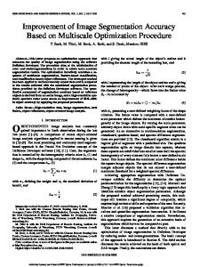
5.4. Numerical results. Numerical results for simultaneous modulation recovery and segmentation are presented in figure 10–12. In the left column of each figure we depict the original image in the first row, the piecewise constant Mumford-Shah-based reconstruction in the middle and the modulation which is applied to the original in the last row. The modulated image is shown in the first row of the right column. The reconstruction obtained by our simultaneous segmentation and modulation recovery scheme and the reconstructed modulation are shown in the second and third row of the right column, respectively. In the first example (see figure 10) the size of the image is 100 × 100 pixels. The applied modulation is σ = x21 + x22 , where (x1 , x2 ) are the cartesian coordinates in the square Ω. The segmentation obtained after the reconstruction of the modulation σ is very close to the original segmentation, as one can see from the middle row of figure 10. The parameter δ for the regularization of σ is δ = 6.10−6 . In the second example (see figure 11) the image size and the applied modulation are as in the previous example. In the segmentation of the reconstructed image a global brightening effect occurs, which is due to an overestimation of the modulation σ. However, all the features of the original image are present in the reconstruction. The parameter δ is equal to δ = 1.10−6 . In the third example (see figure 12) the size of the image is 100 × 100 pixels and the modulation is σ = exp(x1 x2 ) − 1. The result is still satisfying although the exponential modulation is more difficult to reconstruct. The parameter δ is equal to δ = 1.10−6 . 6. Conclusion Numerical results show the efficiency of our topology optimization based modulation recovery and image segmentation algorithm. The scheme requires no particular initialization to obtain an excellent segmentation result. Therefore this technique is completely automatized. The part based on topological sensitivity is highly efficient with respect to CPU-time. We also emphasize that the algorithm for the topological derivative can be easily parallelized, which could result in a dramatic reduction in CPU-time consumption. 7. Appendix 7.1. The level set method. Now we describe the numerical solution of the level set equation (31) and the computation of the extension of vn to the whole domain Ω. Let φ be a level set function, i.e., (50)

Ω = {x | φ(x) < 0},

∂Ω = {x | φ(x) = 0}.

We introduce the nodes Pij , whose coordinates are given by (i∆x, j∆y) where ∆x and ∆y are the discretization steps in the x-direction and ydirection, respectively. Let us also denote by tk = k∆t the discrete time for k ∈ N, where ∆t is the time step. We are seeking for an approximation φkij ' φ(Pij , tk ). Following Osher and Sethian [15, 16], we use the explicit

¨ M. HINTERMULLER AND A. LAURAIN

30

1

1

0.8

0.8

0.6

0.6

0.4

0.4

0.2

0.2

0 150

0 150 120

100

100

120

100

100

80 60

50

40 0

20 0

80 60

50

40 0

20 0

Figure 10. Original image (upper left), modulated image (upper right), segmentation of original image (middle left), segmentation of modulated image (middle right), original modulation (lower left), reconstructed modulation (lower right). upwind scheme (51)

y k y k x k x k φk+1 = φkij − ∆t g(D− φij , D+ φij , D− φij , D+ φij ) ij

where φij − φi−1,j φi+1,j − φij x and D+ φij = ∆x ∆x are the backward and forward approximations of the x-derivative of φ at y y Pij . Similarly we obtain D− and D+ of the y-derivative. The numerical flux is given by (52)

x D− φij =

y y x x g(D− φij , D+ φij , D− φij , D+ φij ) = max(vij , 0) G+ + min(vij , 0) G−

MULTIPHASE IMAGE SEGMENTATION AND MODULATION RECOVERY

1

1

0.8

0.8

0.6

0.6

0.4

0.4

0.2

0.2

0 150

31

0 150 120

100

100

120

100

100

80 60

50

40 0

20 0

80 60

50

40 0

20 0

Figure 11. Original image (upper left), modulated image (upper right), segmentation of original image (middle left), segmentation of modulated image (middle right), original modulation (lower left), reconstructed modulation (lower right). with G+ = G− =

h

h

y y x x max(D− φij , 0)2 + min(D+ φij , 0)2 + max(D− φij , 0)2 + min(D+ φij , 0)2

y y x x min(D− φij , 0)2 + max(D+ φij , 0)2 + min(D− φij , 0)2 + max(D+ φij , 0)2

i1/2 i1/2

and vij = hVext , ni(Pij ) the extended normal velocity at the point Pij as defined in (57) below. This upwind scheme is stable under the CFL condition µ ¶ µ ¶ 1 1 1 (53) max |hVext , ni| ∆t + ≤ . Ω ∆x ∆y 2

,

¨ M. HINTERMULLER AND A. LAURAIN

32

1

1

0.8

0.8

0.6

0.6

0.4

0.4

0.2

0.2

0 150

0 150 120

100

100

120

100

100

80 60

50

40 0

20 0

80 60

50

40 0

20 0

Figure 12. Original image (upper left), modulated image (upper right), segmentation of original image (middle left), segmentation of modulated image (middle right), original modulation (lower left), reconstructed modulation (lower right).

For numerical purposes, the solution φ of the level set equation should not be too flat or too steep. Hence, an instance of φ, which is numerically stable, is the signed distance function which satisfies |∇φ| = 1. Unfortunately, even if the initial data φ0 is given by a signed distance function, the solution φ of the level set equation need not remain close to a distance function, in general. To overcome this difficulty, we perform a reinitialization of φ at time t by computing the stationary state ϕ∞ (x) = limτ →∞ ϕ(τ, x) of the following equation (see [17]): (54) (55)

ϕτ + S(φ)(|∇ϕ| − 1) = 0 in R+ × Ω, ϕ(0, x) = φ(t, x) for x ∈ Ω.

MULTIPHASE IMAGE SEGMENTATION AND MODULATION RECOVERY

33

Here, S is an approximation of the sign function, i.e., S(d) = p

(56)

d d2 + |∇d|2 δ 2

with δ = min(∆x, ∆y). Of course, other choices are possible; see [17] for details. Next we describe the construction of the extension of the normal velocity to the whole domain. Besides the need of a velocity in Ω in the level set equation, another purpose of the extension is to enforce φ to remain a signed distance function. Indeed, if we are able to compute an extended normal velocity Vext such that ∇Vext · ∇φ = 0 in R+ × Ω,

(57)

then it can be shown (see [23]) that the solution φ of the level set equation satisfies |∇φ| = 1. One way to construct the extension Vext satisfying (57) is to solve the following equation up to stationary state (see [15, 17]): (58)

qτ + S(φ)

(59)

∇φ · ∇q = 0 in R+ × Ω, |∇φ| q(0, x) = q0 (x), x ∈ Ω.

Then we take Vext (x) = limτ →∞ q(τ, x). At each iteration k of the previous scheme, we compute the extended normal velocity as the stationary solun ' q(P , tn ) comes from the following upwind tion of (58)-(59). Then qij ij approximation of (58) : (60)

n+1 n − ∆τ qij = qij

x q + min(s nx , 0) D x q [ max(sij nxij , 0) D− ij ij ij + ij y y y + max(sij nij , 0) D− qij + min(sij nyij , 0) D+ qij ] ,

where sij = S(φnij ). We use central differences to compute the approximation nij of the unit normal vector q q ³ ´ n = (nx , ny ) = φx / φ2x + φ2y , φy / φ2x + φ2y at the node Pij . The initial value q0 is equal to vn on the grid points with a distance less than min(∆x, ∆y) to the interface and it is zero elsewhere. Acknowledgement. Both authors are indebted to the anonymous referees for their valuable input which helped to improve the paper. The authors would also like to thank S.L. Keeling (University of Graz) for discussions and for providing a Matlab solver of the fourth-order equation, R. Stollberger and F. Knoll (TU Graz) for providing the 3D medical image data. The authors further acknowledge financial support by the Austrian Ministry of Science and Education and the Austrian Science Fundation FWF under START-grant Y305 ”Interfaces and free boundaries” and the subproject ”Freelevel” of the SFB F32 ”Mathematical Optimization and Applications in Biomedical Sciences”. References [1] T. F. Chan and L. A. Vese, A level set algorithm for minimizing the Mumford-Shah functional in image processing, in: Proceedings of the IEEE Workshop on Variational and Level Set Methods (VLSM ’01), pp. 161-168, Vancouver, BC, Canada, July 2001.

34

¨ M. HINTERMULLER AND A. LAURAIN

[2] M. Delfour and J.-P. Zolesio, Shapes and Geometries. Analysis, Differential Claculus and Optimization, SIAM Advances in Design and Control, SIAM, Philadelphia, 2001. [3] M. Giaquinta, Introduction to Regularity Theory for Nonlinear Elliptic Systems, Birkh¨ auser, Basel–Boston–Berlin, 1993. [4] W. Hackbusch, Elliptic Differential Equations, vol. 18 of Springer Series in Computational Mathematics, Springer Verlag, Berlin, 1992. [5] J.A. Hartigan, Clustering Algorithms, Wiley Series in Probability and Mathematical Statistics, John Wiley & Sons, New York-London-Sydney, 1975. [6] J.A. Hartigan and M.A. Wong, A k-means clustering algorithm, Journal of the Royal Statistical Society (Series C), Applied Statistics, 28 (1979), pp.100-108. [7] L. He and S. Osher, Solving the Chan-Vese model by a multiphase level set algorithm based on the topological derivative, In: Scale Space Variational Methods in Computer Vision, Lecture Notes in Computer Science, pp. 777-788, Springer Verlag, Berlin-New York-Heidelberg, 2007. [8] A. Henrot and M. Pierre, Variation et Optimisation de Formes: Une Analyse G´eom´etrique, No. 48 de Math´ematiques et Applications, Springer, Berlin-New YorkHeidelberg, 2005. ¨ller and W. Ring, A second-order shape optimization approach for [9] M. Hintermu image segmentation. SIAM J. Appl. Math., 64 (2003), pp. 442-467. [10] S.L. Keeling and R. Bammer, A variational approach to magnetic resonance coil sensitivity estimation, Applied Mathematics and Computation, 158 (2004), pp. 53-82. [11] J. MacQueen, Some methods for classification and analysis of multivariate observations, 1967 Proc. Fifth Berkeley Sympos. Math. Statist. and Probability (Berkeley, Calif., 1965/66) Vol. I: Statistics, pp. 281–297 Univ. California Press, Berkeley, California. [12] V. Maz’ya, S.A. Nazarov and B. Plamenevskij, Asymptotic Theory of Elliptic Boundary Value Problems in Singularly Perturbed Domains Vol. 1 and 2, Birkh¨ auser, Basel, 2000. [13] J.-M. Morel and S. Solimini, Variational Methods in Image Segmentation, Progress in Nonlinear Differential Equations and their Applications, 14, Birkh¨ auser Boston Inc., Boston, MA, 1995. [14] D. Mumford and J. Shah Optimal approximations by piece-wise smooth functions and associated variational problems, Commun. Pure Appl. Math., 42 (1989), pp. 577685. [15] S. Osher and R. Fedkiw, Level Set Methods and Dynamic Implicit Surfaces, Springer, Berlin-New York-Heidelberg, 2004. [16] S. Osher and J. Sethian, Fronts propagating with curvature-dependent speed : algorithms based on Hamilton-Jacobi formulation, J. Comp. Phys., 79 (1988), pp. 12-49. [17] D. Peng, B. Merriman, S. Osher, H. Zhao, and M. Kang, A PDE-based fast local level set method, J. Comp. Phys., 155 (1999), pp. 410-438. [18] J.A. Sethian, Level Set Methods and Fast Marching Methods, Cambridge University Press, second edition, Cambridge, 1999. ˙ [19] J. SokoÃlowski and A. Zochowski On the topological derivative in shape optimization, SIAM J. Control Optim., 37 (1999), pp. 1251-1272. [20] J. SokoÃlowski and J.-P. Zolesio, Introduction to Shape Optimization, vol. 16 of Springer Series in Computational Mathematics, Springer, Berlin-New York-Heidelberg, 1992. [21] L. A. Vese and T. F. Chan, A multiphase level set framework for image segmentation using the Mumford and Shah model, International Journal of Computer Vision, 50 (2002), pp. 271-293. [22] S.J. Wright, Primal-Dual Interior-Point Methods, SIAM Publications, Philadelphia, PA, 1997. [23] H.K. Zhao, T. Chan, B. Merriman, and S. Osher, A variational level set approach to multi-phase motion, J. Comp. Phys., 122 (1996), pp. 179-195. [24] W.P. Ziemer, Weakly Differentiable Functions, Graduate Texts in Mathematics, Springer, New York, 1989.

MULTIPHASE IMAGE SEGMENTATION AND MODULATION RECOVERY

35

¨ ller, Humboldt-University of Berlin, Department of MatheM. Hintermu matics, Unter den Linden 6, D-10099 Berlin, Germany, and Karl-FranzensUniversity of Graz, Department of Mathematics and Scientific Computing, Heinrichstrasse 36, A-8010 Graz, Austria E-mail address: [email protected] A. Laurain, Karl-Franzens-University of Graz, Department of Mathematics and Scientific Computing, Heinrichstrasse 36, A-8010 Graz, Austria E-mail address: [email protected]