Multiple Class Machine Learning Approach for Image Auto-Annotation Problem Halina Kwasnicka, Mariusz Paradowski Wroclaw University of Technology, Institute of Applied Informatics halina.kwasnicka,
[email protected] Abstract Image auto-annotation problem becomes more and more popular research topic. Possible applications of auto-annotation methods range from Internet search engines to medical analysis software. The important aspect is that efficient image auto-annotation systems can eliminate the need of annotating huge collections of images manually, which is the only solution today. Most of the methods available in the literature do not use supervised machine learning as the key component. Recent researches show that supervised machine learning can successfully compete with existing approaches. This paper presents a novel image auto-annotation algorithm based of supervised machine learning with the use of C4.5 classifiers.
1. Introduction This paper presents a novel approach for auto-annotation problem with the usage of supervised machine learning techniques. Unsupervised, state of the art techniques are compared to the ones proposed by the authors. In the early days of the image auto-annotation, several algorithms have been presented. Among others, Mori proposed a cooccurence model in [1]. Various translation models, originally used in automatic translation problem are also used in image annotation [2, 3]. Several unsupervised learning approaches for the image auto-annotation problem have also been presented. CMRM method uses clustering algorithm to generate blob tokens [4]. Those blob tokens are used as an intermediate dictionary for the purpose of generating annotations. An approach based on SOM neural network is used in the PicSOM system [5]. CRM [6] and MBRM [7] use feature values directly, together with kernel based techniques as a distance measure. This approaches proves to be very effective and those methods are currently state of the art methods for the image auto-annotation problem. DIMATEX [8] uses a dichotomic clustering for the purpose of speeding up the process, FastAN [9] uses discrete
measures instead of kernel calculation, which is computationally very expensive. Both DIMATEX and FastAN are fast methods and focus mainly on the efficiency. There are also several other approaches. GAP [10] method represents the auto-annotation problem as a graph and uses graphbased techniques. A supervised learning approach based on SVM is discussed in [11]. Mix-hier [12] method uses supervised machine learning with M-ary classifiers, which are also used in the presented method. The paper is organized as follows. The second section describes the proposed method. The third section focuses on the experimental results, the fourth section presents a discussion of the method and the results.
2. BML and MCML methods This section introduces the novel image auto-annotation method proposed by the authors. It is a supervised machine learning method, based on the C4.5 classifiers, although other classifiers may also be used without any difficulty. During our experiments we have found out a couple of important issues, that needed to be explored and revised. As the result of our work, the proposed approach addresses the following issues: • Generation of the training sets • Automatic tuning of the parameters to achieve the expected word recall The method consists of a training phase and a processing phase. The result of the training phase is a set of classifiers, generated for every word in the available word dictionary. Additionally, a set of balancing factors is calculated to improve the annotation results. Training phase is divided into the following steps: 1. Creation of the training set from annotated image data 2. Training of the classifiers 3. Calculation of the balancing factors The result of the processing phase in an annotation for the input image. Processing phase is divided into three steps:
1. Classification of every image region using trained classifiers 2. Scoring of the words using an averaging method 3. Generation of an annotation from scoring In the next sections authors present two algorithms for the image auto-annotation problem. The first one, called Binary Machine Learning (referred as BML) is based on binary classification and is a simpler approach. The second one, called Multiple Class Machine Learning (referred as MCML) is the method, for which authors have achieved best results. It is worth mentioning that the key issues, pointed out by the authors, are addressed in both of those methods.
2.1. Training phase Training phase of the method is responsible for creating W classifiers. Each of those classifiers is a major classifier for one of the words in the dictionary (of size W ). This is the most time consuming part of the algorithm. Binary approach (BML) The first proposed method is based on binary classification. Only two classes are considered: a feature vector is a positive example for a word (YES class) and a feature vector is a negative example for a word (NO class). Every of the BML classifiers is responsible for exactly one word from the annotation dictionary. This is an efficient approach for well-annotated image sets, but for weakly-annotated image sets this proves to be not enough efficient. When a word is not present in the annotation in a weakly-annotated dataset it does not mean that the concept represented by this word is not present in the image. It usually means, that it does not provide any important information about the content of the image. The key weakness in this approach is that all training examples with the NO class are used in a inefficient way. It is used during the classifier training process, but it does not have any direct influence on the result generation process itself. Multiple class approach (MCML) Multiple Class Machine Learning is an extension to Binary Machine Learning. It uses the information contained in the training set in a more efficient way. Each of the W classifiers is a major classifier for one word from the available word collection. The key difference is that each of these classifiers is responsible for classifying all W words. As a result, we receive W classifiers, every with W possible output classes. When training each of the classifiers is performed with with the same dataset, W identical classifiers will be received. To receive distinct classifiers, training set for each classifier must be generated in an distinct way. On the other hand, to receive maximum performance all training examples should be shown during the training of every classifier.
In case of MCML method it is not possible to train the classifiers without the proposed changes in the set construction algorithm. 2.1.1. Training set construction When training a classifier for word w special emphasis is put on positive training instances. A positive instance for a classifier of word w is the instance in which word w is present in the annotation. If word w is not present in the annotation, training instance is considered a negative instance. Having a set of n instances, where p is the number of positive instances, containing word w and q negative examples, not containing word w we balance the number of positive and negative examples to be almost equal. When p < q, more positive examples must be shown during the training to reach the balance, when p > q more negative examples must be shown during the training. Dataset balancing is done by duplicating positive or negative examples in the training set. In case of MCML approach positive instance for word w receives word w as the resulting class. Negative instance for word w receives as the resulting class one of the words that are in the instance description. The word is randomly selected, uniform distribution is used. Algorithm used for creating training set in MCML method is shown in Figure 1. Algorithm B UILD T RAINING S ET MCML(W, I) Input: Word dictionary W , Training instances I Output: Training set T 1. for every word w ∈ W 2. do p ←number of positive instances in I for w 3. q ←number of negative instances in I for w 4. t ←total size of I 5. Tw = ∅ 6. rp = bmin(0.5t/p, 1) + 0.5c 7. rq = bmin(0.5t/q, 1) + 0.5c 8. for every instance i ∈ I 9. do if w ∈ i 10. then classi ←w 11. for x = 1 to rp 12. do Tw = Tw ∪ i 13. else classi ←random word from i 14. for x = 1 to rq 15. do Tw = Tw ∪ i Figure 1. Algorithm for building a training set in the MCML method.
In case of BML approach, positive instance received YES output class and negative instance receives NO class. Algorithm used for creating training set in BML approach is shown in Figure 2.
Algorithm B UILD T RAINING S ET BML(W, I) Input: Word dictionary W , Training instances I Output: Training set T 1. for every word w ∈ W 2. do p ←number of positive instances in I for w 3. q ←number of negative instances in I for w 4. t ←total size of I 5. Tw = ∅ 6. rp = bmin(0.5t/p, 1) + 0.5c 7. rq = bmin(0.5t/q, 1) + 0.5c 8. for every instance i ∈ I 9. do if w ∈ i 10. then classi ←YES 11. for x = 1 to rp 12. do Tw = Tw ∪ i 13. else classi ←NO 14. for x = 1 to rq 15. do Tw = Tw ∪ i Figure 2. Algorithm for building a training set in the BML method.
The largest disadvantage of this method is a large training time. This is caused by the number of possible output classes in the classifier. 2.1.2. Training the classifiers After the data has been prepared, next part of training phase is responsible for training the classifiers. In the proposed approach C4.5 decision tree is used. Other classifiers have also been tested, but both training and processing efficiency and quality of the results prove to be very good for C4.5 classifier. Additionally, C4.5 produces a set of rules, which can be used as a base for construction rule-based image analysis systems. 2.1.3. Calculation of the balancing factors After the classifiers are trained balancing factors are calculated. This requires another creation of the training set and another process of classificator training. In this case, using a part of the training data. First half of the training data is used as a training set. Second half of the training data is used as a test set. Modulo 2 method is used to split the data. The algorithm for the calculation of balancing factors is presented in Figure 3.
2.2. Processing phase After an unannotated image is segmented, each of the regions R is classified by each of the W available classifiers. The results given by the classifiers require further processing. The classification gives us W R answers, which needs to be combined into an image annotation. Combination of the classifier results can be done using two techniques:
Algorithm C ALCULATE BALANCING FACTORS(W, I) Input: Word dictionary W , Training instances I Output: Balancing factors D 1. I1 ←first part of instances from I 2. I2 ←second part of instances from I 3. T = BuildTrainingSet( W , I1 ) 4. BuildClassifiers( T ) 5. for every word w ∈ W 6. do Dw = 1 7. repeat 8. for every image i ∈ I2 9. do annotate image i using factors D 10. for every word w ∈ W 11. do rw ←calculate recall for word w 12. ew ←expected recall for word w 13. xw = min(rw − ew , 0) 14. b ←word with highest xw 15. decrease dw 16. until expected xw reached Figure 3. Algorithm for calculation of the balancing factors used in the MCML and BML methods.
• Simple averaging, which can be seen as a naive method • Balanced averaging (BA) 2.2.1. Simple averaging Calculating the word score (please note that we do not use the term probability because a not normalized value is used) using the simple averaging for a word w can be expressed as:
sw =
R X
cw r,
(1)
r=1
where cw r is equal to 1 if the classifier w has answered positive about word w in region r and 0 otherwise, R represents the number of image segments. Single averaging leads to a major problem. Images are too often annotated with a limited subset of words. When word recall is taken into consideration, frequent words (e.g. sky) are generated too often comparing to the expected annotation results. Together, with the fixed length of the annotation this leads to a problem of almost zero recall for less frequent words. 2.2.2. Balanced averaging (BA) As pointed out before, simple averaging tend to annotate images with the most frequent words. To address this problem, authors introduce balanced averaging. Score for a word w with the use of balanced averaging can be expressed as:
• average per-word recall sw = dw
R X
cw r
(2)
• per-word precision, recall and E score for single words
r=1
where, dw is a balancing factor for a word w calculated on the base of expected word recall. Balancing factors dw are calculated during training phase by presented greedy algorithm (Figure 3). 2.2.3. Annotation of the image After the calculation of all word scores, image annotation is built. Length of the annotation is known a priori and is equal to the length of the original length of the annotation. For an image with r words used in the original annotation, r words with the maximum scores sw are taken as the annotation. As mentioned before, training time of the method is large, but processing time for one image is lower than in many of the unsupervised learning methods.
3. Results This section of the paper presents the experiments authors have performed and the achieved results. All experiments have been performed of three datasets: • MGV 2005, constructed by authors [9], contains 751 images and 74 words • ICPR 2004, a benchmark image database, available in the Internet at [13], contains 1109 images and 407 words • ECCV 2002, based on COREL image database, available in the Internet at [14], contains 5000 images and 374 words MGV 2005 and ICPR 2004 datasets have been segmented using 5x5 Grid approach. Details about the segmentation are given in [9]. Grid segmentation, much simpler than Normalized–Cuts algorithm, proves to be a much more effective data source for the image auto-annotation problem. ECCV 2002 has been segmented using the Normalized–Cuts algorithm. For the purpose of comparison with methods presented in another papers, segmentation and feature values are taken directly from ECCV 2002 dataset. As there are many quality measures available in the literature for the image auto-annotation problem, results have been calculated for several of those measures to make comparison and discussion more conclusive. Definitions and ideas behind those measures have been given, among others in [3, 5, 15]. The following ones are used in the paper: • average normalized score • average accuracy • average per-word precision
Figure 4. Results for the ECCV dataset. Mean per-word recall and precision are calculated for best 60 and all words in the dataset.
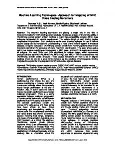
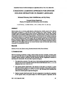
The results from the experiments on the ECCV dataset are shown in Figure 4. Presented method achieved much better results than CRM and CMRM in average normalized score quality measure. It proves to be much more effective method when quality of an annotation is considered. Similar, better results are achieved also for average accuracy measure, as it is a weaker version of normalized score. Higher results are also reported for mean per-word recall and mean per-word precision for 60 best words. For the whole set of 260 words, mean per-word precision and mean per-word recall is better than in CMRM and similar to CRM, which is seen as one of the state of the art methods. Words with the lowest (best) value of E score from the ECCV dataset are presented in Table 1. Highest ranked words with E score are not the most frequent words. This shows that the proposed MCML+BA method is able to effectively annotate images with less frequent word. Similar results are reported for two other tested datasets MGV and ICPR. Results, measured using normalized score are shown in Figures 5 and 6. All dataset splits and experiment average is presented. Dataset splits are created using 1/4 − 3/4 validation. In every case, proposed MCML+BA method gives the best results. Figure 7 gives the results for MGV dataset and Figure 8 shows the results for ICPR dataset measures with various quality measures. Shown values are an average from every dataset split. Additionally, for each of the dataset splits, MCMR performed better than CRM in terms of normalized score, accuracy and mean perword recall and precision for best annotated words. To conclude, in all cases, results measured with average normalized score, average accuracy, mean per-word recall
Word buddha mosque sphinx whales formula cat pillar polar tiger mare swimmers tracks foals pool sun runway black flowers face reefs cars jet horses nest fox
Precision 1.00 1.00 1.00 1.00 1.00 0.76 0.75 0.83 0.69 0.64 0.63 0.66 0.52 0.55 0.52 0.50 1.00 0.58 1.00 0.50 0.56 0.59 0.50 0.50 0.80
Recall 1.00 1.00 1.00 1.00 1.00 0.90 0.90 0.76 0.90 1.00 0.87 0.72 1.00 0.90 0.90 1.00 0.50 0.77 0.50 1.00 0.82 0.68 0.83 0.71 0.44
Expected 1 1 1 1 4 11 10 13 10 9 8 11 9 11 10 1 2 27 2 5 17 19 12 7 9
E score 0.00 0.00 0.00 0.00 0.00 0.16 0.18 0.19 0.21 0.21 0.26 0.30 0.30 0.31 0.33 0.33 0.33 0.33 0.33 0.33 0.33 0.36 0.37 0.41 0.42
Figure 6. Results for the ICPR dataset. Normalized score for every dataset split and an average result.
Table 1. Per-word precision and recall for a set of words with the best E score using MCML+BA. Figure 7. Results for the MGV dataset. Mean per-word recall and precision are calculated for best 20 and all words in the dataset.
method, than the results reported for CRM and CMRM methods. Only for mean per-word recall and precision for all words measures are in some cases similar, and in some cases worse than CRM, but in all cases are better than CMRM.
4. Summary Figure 5. Results for the MGV dataset. Normalized score for every dataset split and an average result.
and precision for best words are better for the proposed
For last few years there have been a major research for unsupervised auto-annotation techniques, but only minor for supervised machine learning techniques. We have shown, that proposed technique, which is based on supervised learning can successfully compete with the state of the art unsupervised learning approaches. To summarize, the key aspects of the proposed method are:
Figure 8. Results for the ICPR dataset. Mean per-word recall and precision are calculated for best 60 and all words in the dataset.
• Generation of the training dataset, in a way to balance positive and negative examples (applies both to binary and multiple class approach), • Balanced averaging, that handles problems with too high recall for frequent words and too low recall for less frequent words (applies both to binary and multiple class approach), • Usage of multiple output classes instead of binary approach. The best version of the method (MCML+AB) provides better results for all tested datasets with normalized score and accuracy quality measures in comparison to CRM. It gives similar results for mean per-word precision and recall for a subset of best words (20 and 60 words, depending on the dataset) but proves to be a equal or less effective for mean per-word precision and recall in the whole subset. The proposed method gives much better results than CRM on the most difficult and largest dataset used – Corel dataset. Further research will focus on training set construction techniques, because it can be the key issue for even further improvement of the results. Next area of research will focus on advancing the method of processing the results of the annotation. The goal of further research is to increase the perword precision and recall for all words in the dataset. Additionally, we plan to use discussed methods in the medical analysis domain for the purpose of semi-automatic diagnosing from images.
References [1] Mori Yasuhide, Takahashi Hironobu, Oka Ryuichi: Image-toword transformation based on dividing and vector quantizing
images with words. In Proceedings of the International Workshop on Multimedia Intelligent Storage and Retrieval Management, 1999. [2] Barnard K., Duygulu P., Forsyth D., de Freitas N.: Object Recognition as Machine Translation - Learning a Lexicon for a Fixed Image Vocabulary, In Proc. of ECCV’2002. [3] Barnard K., Duygulu P., Forsyth D., de Freitas N., Blei D. M., Jordan M. I.: Matching Words and Pictures, Journal of Machine Learning Research 3. [4] J. Jeon, V. Lavrenko and R. Manmatha.: Automatic Image Annotation and Retrieval using Cross-Media Relevance Models, In Proceedings of the ACM SIGIR Conference on Research and Development in Information Retrieval, pp. 119-126, 2003. [5] Ville Viitaniemi and Jorma Laaksonen: Keyword-Detection Approach to Automatic Image Annotation, In Proceedings of 2nd European Workshop on the Integration of Knowledge, Semantic and Digital Media Technologies (EWIMT 2005), London, UK, November 2005. [6] Lavrenko V., Manmatha R., Jeon J.: A Model for Learning the Semantics of Pictures, In Proc. of NIPS’03. [7] S. L. Feng, R. Manmatha and V. Lavrenko: Multiple Bernoulli Relevance Models for Image and Video Annotation, 2004 IEEE Computer Society Conference on Computer Vision and Pattern Recognition (CVPR’04) - Volume 2 pp. 1002-1009. [8] Glotin H., Tollari S.: Fast Image Auto-Annotation with Visual Vector Approximation Clusters, CBMI 2005. [9] Halina Kwasnicka, Mariusz Paradowski: Fast Image AutoAnnotation with Discretized Feature Distance Measures, Machine Graphics and Vision, 2006 (in printing). [10] Pan J., Yang H., Faloutsos C., Duygulu P.: GCap: Graphbased Automatic Image Captioning, In Proceedings of the 4th International Workshop on Multimedia Data and Document Engineering (MDDE 04), in conjunction with Computer Vision Pattern Recognition Conference (CVPR 04), 2004. Washington DC, July 2nd 2004. [11] Cusano, C., G. Ciocca, and R. Schettini: Image annotation using SVM, In Proceedings of Internet imaging IV, Vol. SPIE 5304. 2004. [12] Gustavo Carneiro, Nuno Vasconcelos.: Formulating Semantic Image Annotation as a Supervised Learning Problem, Computer Vision and Pattern Recognition, 2005. CVPR 2005. IEEE Computer Society Conference on Volume 2, 20-25 June 2005 Page(s):163 - 168 vol. 2. [13] ICPR 2005 image dataset, http://www.cs.washington.edu/research/imagedatabase/ groundtruth/ [14] ECCV 2002 image dataset, http://kobus.ca/research/data/eccv 2002/index.html [15] Halina Kwasnicka, Mariusz Paradowski: A Discussion on Evaluation of Image Auto-Annotation Methods, 2006 (in review).