Institute of Technology, P.O. Box 4, Klong Luang, Pathumthani 12120, Thailand. 39 ... a chain and both operations belong to job Ji, then there is no Oik with Oip â Oik .... colony may be guided by different candidate list strategies and heuristic ...
Chapter 4
Multiple-Colony Ant Algorithm with Forward–Backward Scheduling Approach for Job-Shop Scheduling Problem Apinanthana Udomsakdigool and Voratas Kachitvichyanukul
4.1 Introduction The job-shop scheduling problem (JSP) is one of the strongly nondeterministic polynomial-time hard (NP-hard) combinatorial optimization problems and is difficult to solve optimality for large-size problems. For practical purposes, several approximation algorithms that can find good solutions in an acceptable time have been developed. Most conventional ones in practice are based on priority dispatching rules (PDRs). In recent years ant colony optimization (ACO) has been receiving attention in solving scheduling problems including the static and dynamic scheduling problems. The successful applications of the ant algorithm to solve the static problem were founded in the single-machine weighted tardiness problem (Gaen´e et al. [1], Gravel et al. [2]), the flow-shop scheduling problem (Shyu et al. [3], Ying and Liao [4]), the open-shop scheduling problem (Blum [5]), and the resource constraint project scheduling problem (Merkle et al. [6]). The application to JSP has proven to be quite difficult. The first group of researchers (Colorni et al. [7]) that applied ACO algorithm to solve the JSP was far from reaching state-of-the-art performance. Later Blum and Sampels [8] developed the ant algorithm for shop scheduling, and the results indicate that their algorithm works well when applied to the open-shop problem. In Udomsakdigool and Kachitvichyanukul [9] the forward–backward scheduling approach is applied in the single-colony ant algorithm, and they found that this approach improves the solution in many problems. Recently, Udomsakdigool and
Apinanthana Udomsakdigool The department of Industrial Engineering Technology, College of Industrial Technology, King Mongkut’s Institute of Technology North Bangkok, 1518 Pibulsongkram Road, Bang Sue, Bangkok, 10800, Thailand Voratas Kachitvichyanukul The Department of Industrial System Engineering, School of Engineering and Technology, Asian Institute of Technology, P.O. Box 4, Klong Luang, Pathumthani 12120, Thailand
39
40
Apinanthana Udomsakdigool and Voratas Kachitvichyanukul
Kachitvichyanukul [10] introduced the multiple-colony ant algorithm to find the JSP solution. This approach uses more than one colony of ants working cooperatively for the solution, and the result clearly shows that most scheduling problems can be improved. This paper proposes the new method of ACO to solve the JSP. In this method, forward–backward scheduling and multiple–colony approach are introduced. In the proposed ant algorithm, each colony contains two types of ants that construct the solutions in order of precedence and in the reversing order of precedence of processing sequences. These two types of ants exchange the information via modifying the pheromone trail in the same pheromone matrix. Each colony is characterized by the information they use to guide their search, i.e., each colony is forced to search in different regions of search space and cooperate to find good solutions by exchanging information among colonies. The proposed algorithm is investigated for its potential in solving the benchmark instances available in OR-Library (Beasley [11]). This paper is organized as follows. In the Section 4.2, a definition of the JSP, a graph-based representation, the general concept of ACO, the memory requirement for ant and colony, the hierarchical cooperation in multiple colonies, and the backward scheduling approach are given. The descriptions and the features in the proposed ant algorithm are presented in Section 4.3. The computational results on benchmark problems are provided in Section 4.4. Finally the conclusion and recommendation for further study are presented in Section 4.5.
4.2 Problem Definition and Graph-Based Representation 4.2.1 Problem Definition The n × m JSP can be defined as a set J of n jobs {Ji }ni=1 to be processed on a set M of m machines {M j }mj=1 . Each job Ji composes of a set of operations {Oi j }mj=1 to be performed on machines for an uninterrupted processing time pi j .. The processing order of operations required for each job represents the predetermined given order of job through the machines (precedence constraint). If the relation Oip → Oiq is in a chain and both operations belong to job Ji , then there is no Oik with Oip → Oik or Oik → Oiq , and Oip has to be finished before Oiq can start. Each machine can process at most one job, and each job can be processed by only one machine at a time (machine constraint). The objective is to determine the starting time Si j for all operations in order to minimize the makespan Cmax while satisfying all precedence and machine constraints as described mathematically in equation (4.1) and the inequalities (4.2) and (4.3), respectively. minCmax = min{max(Sij + pij ) : ∀Ji ∈ J, ∀M j ∈ M},
Oi j ∈ O
(4.1)
4 Multiple-Colony Ant Algorithm with Forward–Backward Scheduling
41
subject to Si j ≥ Sik + pik
when Oik → Oi j,,
(4.2)
(Si j ≥ Sk j + pk j ) ∨ (Sk j ≥ Si j + pi j ).
(4.3)
4.2.2 Graph-Based Representation Every instance of the JSP can be formulated using a graph-based representation called a disjunction graph G = (O,C, D), where O is the set of all nodes (processing operations), C is a set of conjunctive directed arcs, and D is a set of disjunctive undirected arcs that represents the machine constraint of operations belonging to different jobs. C corresponds to the precedence relationship between operations of a single job. Thus, operations belonging to the same job are connected in sequence. The operations of jobs that are processed on the same machine are connected pairwise in both directions. Two additional fictitious nodes, the source (the predecessor of the first operation of every job) and the sink (the successor of the last operation of every job) of the zero processing time are added to the set. A path P is defined as an acyclic sequence of total operations that represent the possible solution of the instance. The makespan of a schedule is equal to the longest path from source to sink in P. This path is called a critical path, and the operations that it passes through are called critical operations. An example the job-shop problem is introduced here to explain the ideas. The instance consists of nine operations that are partitioned into three jobs and have to be processed on three machines. The detail of the example problem is shown in Table 4.1. The disjunctive graph of the example is presented in Fig. 4.1, where dotted lines represent the conjunctive directed arcs of machines and the bold line represents the undirected arcs of jobs. When the processing order is determined, the direction of arcs will be selected in such a way that P is acyclic. For example, the processing order of operations are selected based on the most work remaining criterion; choose one that has the highest work remaining. The sequence of operations of P is to be {source → O1 → O7 → O4 → O2 → O8 → O5 → O3 → O6 → O9 → sink} The Gantt chart of P is presented in Fig. 4.2., and it can be observed that the critical path passes through {O1 → O8 → O5 → O6 } the makespan is equal to 13 units of time.
Table 4.1 The detail of an example problem Operation Job1 Job2 Job3
O1 O4 O7
O2 O5 O8
Machine O3 O6 O9
M3 M2 M1
M2 M3 M3
Process time M1 M1 M2
3 3 3
4 3 5
3 2 1
42
Apinanthana Udomsakdigool and Voratas Kachitvichyanukul
Fig. 4.1 Disjunctive graph of the example problem
4.2.3 The General Concept of ACO Algorithm The ACO algorithm is a metaheuristic inspired by the foraging behavior of real ants. This behavior is the basis for local interaction of each ant, which leads to the emergence of shortest path. In the ACO algorithm a finite-size colony of artificial ants collectively searches for good-quality solutions to the problem under consideration. There are two main components in an ant algorithm: the construction of solution and the update of pheromone trail. In the construction step, each ant constructs a feasible solution by using the incremental constructive approach. Each ant builds a solution, starting from an initial state moving through a sequence of neighboring states, by applying a stochastic local search policy directed (a) by private information of an ant and (b) by publicly available pheromone trails accumulated by all the ants from the beginning of the search process and a priori problem-specific local information. After they complete their solutions, the pheromone values are updated depending on the quality of the solutions; the better the solution, the stronger the pheromone value. This process serves as a positive feedback mechanism for the sharing of information about the quality of the solution found, and the evaporation process allows the
Fig. 4.2 Gantt chart of the solution of an example problem
4 Multiple-Colony Ant Algorithm with Forward–Backward Scheduling
43
ants to forget the regions that do not contain a solution with high quality. After the ants repeat this procedure for a certain number of iterations, the path that has strongest pheromone value will become the dominant solution. This solution expresses a shortest path through the states of the problem that emerged as a result of the global cooperation among all ants of the colony (for more detail, see Dorigo and St¨utzle [12]).
4.2.4 Memory Requirement for Ant and Colony In an ant algorithm, a finite number of ants in a colony search for solutions independently. The ants share their experience by updating the pheromone matrix, and through this cooperative behavior, the best solution will emerge after a number of iterations. To implement the ant algorithm, the basic data structures have to be defined. These structures must allow data storage for the problem instance and the pheromone trail, as well as represent each individual ant. To manage the solution construction, each ant has its own local memory to store the past history of movement along with useful information to compute the goodness of the move. Moreover, it can play a fundamental role in managing the feasibility of the solutions. Once each ant has accomplished its task, the information sharing among individuals in the colony is achieved through the update of the common memory called the pheromone matrix. The required data structure is shown in Fig. 4.3. The pheromone trail matrix collects the pheromone trail, which represents a long-term memory about the search experience of the colony. The pheromone trails change over time depending on the pheromone updating rule. The heuristic information matrix collects heuristic information for possible exploitation of problem-specific knowledge. The heuristic information used by the ant may be static or dynamic. In the static case the values of heuristic information are computed once at the initialization time and remain unchanged throughout the run. An example is the use of process time as heuristic information; the value is unchanged. In contrast, the heuristic information for the dynamic case depends on the partial solution constructed so far and therefore has to be recomputed at each step of an ant’s journey. An example is the use of heuristic information based on remaining work time; the value varied depends on the partial solution constructed. Accordingly, each ant has its own memory to manage the solution construction. This memory is equipped with four lists: The unvisited list contains the unscheduled operations. The allowable list contains the operations that do not violate the technological constraints. To reduce the search space in the allowable list and to guide an ant to search in the high-quality region, some constraints are imposed on the ant walk. The operations with respect to those constraints are kept in the candidate list. Finally, the visit list is used to keep the selected operation or the sequence of moves by an ant.
Apinanthana Udomsakdigool and Voratas Kachitvichyanukul
F
tF
tF
tF
1
...
2
...
tFF
O1
O2
O3
O4
O5
O6
O7
O8
O9
S
1
2
hSS hS1 hS2 h1S h11 h12 h2S h21 h22
... F ... hSF ... h1F ... h2F ...
S
...
tSF t1F t2F
...
F
... ... ... ... ...
2
tS2 t12 t22
...
2
1
tS1 t11 t21
...
1
S
tSS t1S t2S
...
S
Heuristic Information Matrix From/ To
...
Pheromone Trail Matrix From/ To
...
44
hFS hF1 hF2 ... hFF
F
Colony Memory S
Ant Memory
O1
O2
O3
Allowable list O1
O4
O7
Candidate list O1
O4
Unvisit list
...
F
F
Visit list
S start or source node, F finish or sink node Fig. 4.3 Memory requirements for ant and colony: (S) start or source node, (F) finish or sink node
4.2.5 Hierarchical Cooperation in Multiple Colonies The basic idea of multiple colonies is to coordinate the activity of different ant colonies; each of them optimize a makespan of the problem instance. Ants in multiple colonies cooperate in two levels: high-level cooperation and low-level cooperation. In the low-level cooperation, individuals in the colony cooperate to find the best solution. In the high-level cooperation, each colony uses the useful information collected from many colonies to find the best solution. The hierarchical level of cooperation in multiple colonies is shown in Fig. 4.4. In the proposed technique, the colonies work by using both the individual, or local, pheromone matrix and the overall, or global, pheromone matrix. As shown in Fig. 4.5. the local pheromone matrix stores the information for each colony. In contrast, the global pheromone matrix serves the role of global memory, collecting the information from colonies. Ants in each colony perform the same task, that is, to find the solution in the search space. The exploration of the search space in each colony may be guided by different candidate list strategies and heuristic information. When the ants construct the solution, they use the combination of information from both global pheromone trail and local pheromone trail. The local pheromone trails are updated separately, but the global pheromone is updated only by the best of all colonies.
4 Multiple-Colony Ant Algorithm with Forward–Backward Scheduling
45
Fig. 4.4 Hierarchical level of cooperation in multiple colonies
In summary, the multiple-colony ant algorithm is the technique in which ants cooperate to find good solutions by using both the local experience within a colony as well as shared information among colonies.
4.2.6 Backward Scheduling Approach In general, a given problem of the job-shop scheduling problem can be converted to a problem equivalent to the original one, called reversed problem. The reversed problem assumes that the operations must be processed in the reverse order of the original problem; that is, the predecessors of each operation are considered as its successors. If the reversed problem is used, however, the resulting schedule should
Fig. 4.5 The pheromone trail matrix and the cooperation in multiple colonies
46
Apinanthana Udomsakdigool and Voratas Kachitvichyanukul
Fig. 4.6 Gantt chart of the reverse of P with left shift procedure
be reversed back to the regular time frame after it is solved. The start time and the completion time of a job in the original problem are related to the completion time and the start time of the job in the reversed problem, respectively. It sometimes happens that a reversed problem is easier to solve than the original. For example, the criterion to select the processing order of operations of the example problem is the same but selected in the reversed order of the precedence constraint. Hence, the sequence of operations of P is to be {source → O3 → O9 → O6 → O8 → O2 → O5 → O1 → O7 → O4 → sink}. The reverse of this sequence can be used to form a schedule. If a non-delay schedule is required as a solution, left shift of operations (moving operations to earliest possible time without violating precedence constraints and given order of operations) on each machine must be done at the final step of the backward approach. In this example, the makespan is reduced to 12 units of time. The Gantt chart with reverse sequence of schedule P is illustrated in Fig. 4.6.
4.3 Description of Algorithm In the proposed ant algorithm, hereinafter called MFBAnt, there are at least two heterogeneous colonies characterized by the heuristic information they use to guide their search. In each colony two kinds of ant, forward and backward ants, work for the best solutions. The main steps in MFBAnt include the solution construction and the pheromone updating. In the construction step, the forward ants and backward ants select the operation from a set of allowable operations by applying the two-step random probability transitional rule guided by the pheromone trail and the heuristic information (Dorigo and Gambarella [13]). After the ants complete their solution, a local improvement is performed. Then the two-step pheromone updating, local and global updating rule is performed. The restart process is also applied when the search is trapped in a local optimum. The procedure of MFBAnt is shown in Fig. 4.7. The details of each step are described in the following sections.
4 Multiple-Colony Ant Algorithm with Forward–Backward Scheduling
47
4.3.1 Initialize Pheromone and Parameter Setting The pheromones are initialized with the value drawn as a random number in the interval (0.1, 0.5). The reason behind that is to enforce the diversification at the start of the algorithm. The parameters that control the search are set to the important weight of pheromone trail, α = 1; the important weight of heuristic information, β = 5; the important weight of global pheromone trial, w = 0.7; the pheromone evaporating weight of local and global pheromone matrix, ρl , ρg = 0.1; and the exploitation– exploration weight, q0 = 0.5. The number of ants in each colony is n, the number of total operations is O, the number of forward ants is a f = 0.8O, and the number of backward ants is ab = 0.2O. The algorithm terminates when the total number of iterations reaches 1000. The parameter values of ACO used in this study are the numbers as reported by Udomsakdigool and Kachitvichyanukul [9, 10]. In MFBAnt, three colonies with most work remaining, earliest start time, and earliest finish time as heuristic information are introduced [10]. In the construction step, the forward and backward ants construct the solution in forward and reverse order of precedence constraints, respectively. For backward ants the schedule should be reversed back to the normal time frame after it is solved. The detail of solution construction is described as follows. For all colonies, at each step of solution construction, an ant k selects one operation from a set of candidate operations Ck , that is, a subset of allowable operations Ak that can be scheduled at a construction step by applying probability transitional rule. The selection probability for each operation in the set Ck depends on the two-step random proportional probability transition rule model as follows. While building the solution, the selection of operation by an ant is guided by the pheromone information τ and the heuristic information η . At the construction step of operation i in iteration t, the kth ant selects an operation by taking a random number q. If q ≤ q0 , the operation is chosen according to (4.4). Otherwise, an operation is selected according to (4.5). � ⎧ � ⎪ ⎨arg max[τ k (t)]α [η k ]β if q ≤ q0 , io io jik (t) = (4.4) o∈Cik ⎪ ⎩ J otherwise, where j is the selected operation at the present step of operation i and J is an operation selected from the random proportional transition rule defined as (4.5). ⎧ k α kβ [τ (t)] [η ] ⎪ ⎨ ∑ io[τ k (t)]αio[η k ]β io k (4.5) pio (t) = o∈Cik io ⎪ ⎩ 0 otherwise, where i is the operation at the current step, o is the operation in candidate list, pio is a probability to select operation o for the next step, τio is the pheromone trail between operations i and o, ηio is the heuristic information between operations i and o, and
48
Apinanthana Udomsakdigool and Voratas Kachitvichyanukul
Input: A problem instance of the JSP /∗Step 1: Initialization ∗/ /∗Set parameter values∗/ Set parameters (Nt = tmax , α = αc , β = βc , ρl , ρg = ρc , q0 = q0c , Rn = nmax Nc = c, Nc1 = c1 , Nc2 = c2 , . . . , Ncc = cc , ρg = ρc , w = wc ) /∗Initialize global pheromone value∗/ For each edge (i, j) do Set an initial global pheromone value τi j,g (0) = τ0 End for /∗Initialize local pheromone value∗/ For Nc = 1 to c For each edge (i, j)do Set an initial local pheromone value τi j,l (0) = τ0 End for End for /∗Main loop∗/ /∗Step 2: Solution construction∗/ Set best solution since start algorithm, Ssg (t0 ) = φ For t = 1 to tmax do For Nc = 1 to c do Set best solution of colony c since start algorithm, Ssc (t0 ) = φ Set Best solution of colony c in iteration, Sic (t0 ) = φ For t = 1 to tmax do If forward ant then For k = 1 to a f do /∗Set all lists†∗/ Set Unvisit list, U k = ∀O /∗all operations∗/ Set Visit list, V k = φ Set Allowable list, Ak = φ Set Candidate list, Ck = φ End for For k = 1 to a f do /∗Starting node∗/ Place ant k on the starting node Store this information in V k Delete this operation from U k /∗Build the solution for forward ant∗/ Ant builds a tour step by step until U k = φ by apply the following steps: Ant randomly choose q number, q = rand(0, 1) Choose the next operation j from Ck according to equation (4.4) If q ≤ q0 , Otherwise an operation is selected according to equation (4.5) Keep operation j in V k and delete operation j from U k Compute the makespan Cmax of the sequence, Sk in V k End for /∗Step 3: Local improvement, option∗/ For ant k = 1 to a f do Apply local improvement If an improve Cmax is found then Update Cmax and V k End for Fig. 4.7 Procedure of MFBAnt. a Perform the same step as forward ants, but the solutions are constructed in the reverse order of precedence constraint. b Perform the same step as forward ants
4 Multiple-Colony Ant Algorithm with Forward–Backward Scheduling
49
For ant k = 1 to af do Select best solution of forward ant of iteration t, Si f (t) End for Update the Sif (t) of forward ant Update the Ssf (t) of forward ant End if /∗Backward ant∗/ If backward ant then For k = 1 to ab do /∗Set all lists †∗/ End for For k = 1 to ab do /∗Starting node∗/ ∗ / Build the solution for each ant a∗/ /∗Step 3: Local improvement, option b∗/ End for For ant k = 1 to ab do Select best solution of backward ant of iteration t, Sib (t) End for Reversed back Sib (t) to the forward time frame End if Selected Si (t) ← best(Si f (t), Sib (t)) Update the Sic (t) Update the Ssc (t) /∗Step 4: Update local pheromone matrix∗/ For each edge (i, j) in V k of Sic (t) do Update pheromone trials according to equation (4.8) End for /∗Step 5: restart process for each colony (local pheromone matrix), option∗/ If the restart criteria is reached Apply restart process End if End for Update the Ssg (t) /∗Step 6: Update global pheromone matrix∗/ For each edge (i, j) in V k of Ssg (t) do Update pheromone trials according to the equation (4.9) End for /∗Step 7: restart process for colonies (global pheromone matrix), option∗/ If the restart criteria is reached Apply restart process End if End for Output: Best solution Fig. 4.7 (Continued)
Ci is the set of operations in the candidate list at the step of operation i. In addition, α and β are the parameters that determine the relative importance of the pheromone trail and the heuristic information (α > 0, and β > 0), q is the random number uniformly distributed in [0,1], and q0 ∈ (0,1) is the parameter that determines the relative importance between exploitation and exploration. The pheromone trail between
50
Apinanthana Udomsakdigool and Voratas Kachitvichyanukul
operations i and o is calculated as in (4.6): k k τiok (t) = (1 − w)τio,l (t) + wτio,g (t)
(4.6)
where w is the important weight of global pheromone trail, τio,l is the pheromone trail between operations i and o from the local pheromone matrix, and τio,g is the pheromone trail between operations i and o from the global pheromone matrix. To translate the dispatching rules (most work remaining, earliest start time, and earliest finish time) into heuristic information score, every operation in the candidate list C is normalized. An example of translating the most work remaining into heuristic information scores is shown in (4.7), where ηo is a heuristic information score of operation o, wr is the work remaining time of the job that operation o belongs to.
ηo ←
wr(o) . ∑ wr(o)
(4.7)
o∈C
The selected operation is kept in the visit list V k . Ant repeats the construction step until the set U k , which contains the unscheduled operations, is empty. A sequence Sk of all the operations O in V k (except for the source and the sink) indicates a solution for the job-shop problem. The makespan of the solution can be calculated from the critical path Cp in Sk .
4.3.2 Local Improvement The local improvement plays an importance role in improving the solution, especially in the metaheuristic method. The local improvement procedure explores the best solution from a certain neighborhood of a given schedule and keeps it as the solution. In the ant algorithm, the local improvement is performed after the ants complete their solutions. The local improvement method used in this paper is adapted from Nowicki and Smutinicki [14], which defined a neighborhood solution by moving the operation near the border line of blocks on a single critical path in sequence of processing order. In the first block the last two operations are swapped, and in the last block the first two operations are swapped, respectively. For other blocks between the first and the last blocks, the first two and the last two operations that contain at least two operations are swapped. In Fig. 4.2 there is a single critical path Cp = (O1 , O8 , O5 , O6 ) that decomposes into 2 blocks, B1 = (O1 , O8 , O5 ) and B2 = (O6 ). There is one neighborhood solution that swaps operation O8 and O5 . Sometime in performing the moves, it is possible to end up with a schedule that is not feasible. To cope with this problem, the rearrange technique is introduced. In other words, the operation that violates the precedence constraint will be moved after its predecessor. After the neighborhood search is performed, the sequence with the best makespan is kept as the solution. If this search does not improve the objective, the original solution is kept.
4 Multiple-Colony Ant Algorithm with Forward–Backward Scheduling
51
4.3.3 Pheromone Updating In MFBAnt, the two-step pheromone updating rule is performed. That is, after each colony updates its local pheromone matrix, the global pheromone matrix is updated. In local updating, the solutions from each ant, including forward and backward ants, in the colony are compared, and the best solution is kept as the best solution in iteration. Then this solution is compared with the best solution since the start of the algorithm for their individual colony. The best of these solutions is used to update the local pheromone matrix. For global updating, the best solutions since the start algorithm of each colony are compared with the best solution since the start of all colonies. The best solution among them is used to update the global pheromone matrix.
4.3.3.1 Local Pheromone Matrix Updating In colony c, after all ants complete their solutions, the best solution found in colony c since the start of algorithm, Ssc , is used to update its local pheromone matrix. The rule of pheromone updating is defined in (4.8).
τij,l (t + 1) = (1 − ρl )τij,l (t) + ρl ∆τij,l (t), where
� 1 τi j,l (t) = 0
(4.8)
if (i, j) ∈ tour of Ssc , otherwise.
In equation (4.8), ρl ∈ [0, 1) is the pheromone evaporating parameter for the local pheromone matrix. The minimum pheromone value is set to 0.001. When applying the pheromone updating, the pheromone value that is less than this number is set back to 0.001.
4.3.3.2 Global Pheromone Matrix Updating The information exchange among colonies is done after all colonies finish their solutions. The best solution since the start of all colonies, Ssg , is used to update the global pheromone matrix following the formula given in (4.9).
τi j,g (t + 1) = (1 − ρg )τi j,g (t) + ρg ∆τi j,g (t), where
� 1 τi j,g (t) = 0
(4.9)
if (i, j) ∈ tour of Ssg , otherwise.
In equation (4.9), ρg ∈ [0, 1) is the pheromone evaporating parameter for global pheromone matrix updating. The minimum pheromone value is set to 0.001. When
52
Apinanthana Udomsakdigool and Voratas Kachitvichyanukul
Table 4.2 Results of MFBAnt on benchmark problems Proposed algorithm Problem instance
Size(n × m)
Optimal
FT06 FT10 FT20 LA01 LA02 LA03 LA04 LA05 LA06 LA07 LA08 LA09 LA10 LA11 LA12 LA13 LA14 LA15 LA16 LA17 LA18 LA19 LA20 LA21 LA22 LA23 LA24 LA25 LA26 LA27 LA28 LA29 LA30 LA36 LA37 LA38 LA39 LA40 ABZ5 ABZ6 ORB1 ORB2 ORB5 ORB6
6×6 10 × 10 20 × 5 10 × 5 10 × 5 10 × 5 10 × 5 10 × 5 15 × 5 15 × 5 15 × 5 15 × 5 15 × 5 20 × 5 20 × 5 20 × 5 20 × 5 20 × 5 10 × 10 10 × 10 10 × 10 10 × 10 10 × 10 15 × 10 15 × 10 15 × 10 15 × 10 15 × 10 20 × 10 20 × 10 20 × 10 20 × 10 20 × 10 15 × 15 15 × 15 15 × 15 15 × 15 15 × 15 10 × 10 10 × 10 10 × 10 10 × 10 10 × 10 10 × 10
55 930 1165 666 655 597 590 593 926 890 863 951 958 1222 1039 1150 1292 1207 945 784 848 842 902 1046 927 1032 935 977 1218 1235 1216 1152 1355 1268 1397 1196 1233 1222 1234 943 1059 888 887 1010
Average % deviationa a Average
Best 55 ∗ 930 ∗ 1165
666 ∗ 655 ∗ 597
590 593 926 890 863 951 958 1222 1039 1150 1292 ∗ 1207 ∗ 947 ∗ 784 848 ∗ 848 ∗ 907 1063 ∗ 944 ∗ 1032 ∗ 940 ∗ 989 ∗ 1220 ∗ 1240 ∗ 1247 1162 ∗ 1365 ∗ 1300 ∗ 1439 1224 ∗ 1262 ∗ 1250
Udomsakdigool and Kachitvichyanukul [10]
%D
Time (s)
Best
%D
Time (s)
0.00 0.00 0.00 0.00 0.00 0.00 0.00 0.00 0.00 0.00 0.00 0.00 0.00 0.00 0.00 0.00 0.00 0.00 0.21 0.00 0.00 0.71 0.55 1.63 1.83 0.00 0.53 1.23 0.16 0.40 2.55 0.87 0.74 2.52 3.01 2.34 2.35 2.29
34 162 235 36 36 37 38 36 101 102 101 103 102 236 235 235 238 236 161 160 162 162 161 902 900 898 905 904 8563 8558 8559 8560 8560 12618 12614 12620 12619 12624
55 944 1178 666 658 603 590 593 926 890 863 951 958 1222 1039 1150 1292 1240 977 793 848 860 925 1063 954 1055 954 1003 1308 1269 1328 1162 1411 1334 1457 1224 1298 1269 1239 948 1070 893 897 1022
0.00 1.51 1.12 0.00 0.46 1.01 0.00 0.00 0.00 0.00 0.00 0.00 0.00 0.00 0.00 0.00 0.00 2.73 3.39 1.15 0.00 2.14 2.55 1.63 2.91 2.23 2.03 2.66 7.39 2.75 9.21 0.87 4.13 5.21 4.29 2.34 5.27 3.85 0.41 0.53 1.04 0.56 1.13 1.19
21 70 82 13 14 13 12 14 35 36 36 35 37 80 82 82 88 85 52 54 54 56 55 390 409 384 385 382 3155 3125 3150 3200 3204 3096 2928 3062 3048 2998 72 70 74 70 72 70
0.63%
% deviation is calculated from the same 38 problems, FT06 to LA40.
1.92%
4 Multiple-Colony Ant Algorithm with Forward–Backward Scheduling
53
applying the pheromone updating, the pheromone value that is less than this number is set back to 0.001
4.3.4 Restart Process When the system is trapped in an area of the search space a restart process is performed. There are two types of restart process: local restart process and global restart process. Each colony performs the local restart process if the ants are trapped in a local optimum. All pheromone values in every path in the local pheromone matrix are reinitialized, and the algorithm is started again. The global restart process is performed if the best solution of all colonies since the start of the algorithm is not improved. The pheromone values in every path in the global pheromone matrix are reinitialized, and the algorithm is started again. The restart processes in the global pheromone matrix and the local pheromone matrix are performed separately.
4.4 Experimental Results MFBAnt is tested on benchmark problems that are available from the OR-Library. The algorithm was coded in C and run on a Pentium 4, 2.4-GHz PC with 1 GB of RAM running on a Windows platform. To evaluate the algorithm, each of the problem instances was repeated for 10 trails. The best solution is obtained from 10 trails of this tested algorithm. The percent deviation from the optimal solution is calculated as [(best solution – optimal solution)/optimal solution] ×100. The CPU time is in seconds. The final results are listed in Table 4.2. The results in Table 4.2 illustrate that there are 21 instances, FT06 to FT20, LA01 to LA15, LA17, LA18, and LA23, where the algorithms yielded the optimal solution without using local improvement and restart process. The deviation is less than 1% for the small-size problem and less than 4% for the large-size problem. The average percent deviation is 0.63%. Comparing this with the solutions of 24 problems obtained by Udomsakdigool and Kachitvichyanukul [10], the proposed algorithm yields better solutions in 21 problems, and in 3 problems the solutions are the same. This comparison excludes 14 problems that yield optimal solutions.
4.5 Conclusion and Recommendation 4.5.1 Conclusion This paper presents the new method of the ant algorithm applied to solve the JSP. The proposed algorithm includes the forward–backward scheduling and
54
Apinanthana Udomsakdigool and Voratas Kachitvichyanukul
multiple-colony approach. This algorithm is tested for the performance over the benchmark problems. The experimental result indicates that this method yields excellent performance. The average percent deviation is 0.63%. Comparing with [10], the average percent deviation is 1.92%. It can be concluded that the performance of MFBAnt is achieved by allowing the ants to diversify the search via construction of solutions in the forward and backward directions and to exploit different regions via different heuristic information. In addition, the information exchange among colonies allows them to access the lesson learned by the other colonies.
4.5.2 Recommendation There are many possibilities to further improve the algorithm. First, to achieve an efficient multiple-colony ant algorithm, the strategy for information exchange should be examined. For example, which kind of information should be exchanged? How frequent should the exchanges take place among the colonies? In addition, the execution time may be reduced when parallel implementation is included. Second, in order to improve the efficiency of the proposed algorithm, different local improvement techniques, such as left-shift local search and e-shift, may be combined with ant algorithm, and their performance should be investigated. Finally, to increase the effectiveness and efficiency in the exploration of the search space, strategic use of randomness during an ant’s solution construction of may be considered. However, the appropriate balance between diversification and intensification remains a topic for further investigation.
References 1. C. Gaen´e, W.L. Price, and M. Gravel (2002) Comparing and ACO algorithm with other heuristics for the single machine scheduling problem with sequence-dependent setup times. Journal of the Operational Research Society, 53: 895–906. 2. M. Gravel, W.L. Price, and C. Gagn´e (2002) Scheduling continuous casting of aluminium using a multiple objective ant colony optimization metaheuristic. European Journal of Operations Research, 143: 218–229. 3. S.J. Shyu, B.M.T. Lin, and P.Y. Yin (2004) Application of ant colony optimization for no-wait flow shop scheduling problem to minimize the total completion time. Computer and Industrial Engineering, 47: 181–193. 4. K.C. Ying and C.J. Liao (2004) An ant colony system for permutation flow-shop sequencing. Computers and Operations Research, 31(5): 791–801. 5. C. Blum (2004) Beam–ACO-hybridizing ant colony optimization with beam search: An application to open shop scheduling. Computers and Operations Research, 32(6): 1565–1591. 6. D. Merkle, M. Middendorf, and H. Schmeck (2002) Ant colony optimization for resourceconstrained project scheduling. IEEE Transaction on Evolutionary Computation, 6(4): 53–66. 7. A. Colorni, M. Dorigo, V. Maniezzo, and M. Trubian (1996) Ant system for job-shop scheduling. Belgian Journal of Operations Research, Statistics, and Computer Science, 34(1): 39–54.
4 Multiple-Colony Ant Algorithm with Forward–Backward Scheduling
55
8. C. Blum and M. Sampels (2004) An ant colony optimization algorithm for shop scheduling problems. Journal of Mathematical Modelling and Algorithms, 3: 285–308. 9. A. Udomsakdigool and V. Kachitvichyanukul (2006) Two-way scheduling approach in ant algorithm for solving job shop problems. Industrial Engineering and Management Systems, 5(2): 68–75. 10. A. Udomsakdigool and V. Kachitvichyanukul (2007) Multiple colony ant algorithm for jobshop scheduling problem. International Journal of Production Research, 99999:1: 1–21. (Online link to article URL: http://dx.doi.org/10.1080/00207540600990432). 11. J.E. Beasley (1996) Obtaining test problems via Internet. Journal of Global Optimization, 8(4): 429–433. 12. M. Dorigo and T. St¨utzle (2004 ) Ant colony optimization. The MIT Press, Cambridge, MA. 13. M. Dorigo and L.M. Gambarella (1997) Ant colonies for the traveling salesman problem. Biosystems, 43(2): 73–81. 14. E. Nowicki and C. Smutinicki (1996) A fast table search algorithm for the job-shop problem. Management Science, 42(6): 797–813.