Clustering algorithm for determining community ... - Semantic Scholar

PHYSICAL REVIEW E 74, 016107 共2006兲

Clustering algorithm for determining community structure in large networks Josep M. Pujol,* Javier Béjar, and Jordi Delgado Software Department, Technical University of Catalonia, Jordi Girona 1-3 A0-S106, 08034, Barcelona, Spain 共Received 10 February 2006; revised manuscript received 15 March 2006; published 17 July 2006兲 We propose an algorithm to find the community structure in complex networks based on the combination of spectral analysis and modularity optimization. The clustering produced by our algorithm is as accurate as the best algorithms on the literature of modularity optimization; however, the main asset of the algorithm is its efficiency. The best match for our algorithm is Newman’s fast algorithm, which is the reference algorithm for clustering in large networks due to its efficiency. When both algorithms are compared, our algorithm outperforms the fast algorithm both in efficiency and accuracy of the clustering, in terms of modularity. Thus, the results suggest that the proposed algorithm is a good choice to analyze the community structure of medium and large networks in the range of tens and hundreds of thousand vertices. DOI: 10.1103/PhysRevE.74.016107

PACS number共s兲: 89.75.Hc, 05.10.⫺a, 87.23.Ge, 89.20.Hh

Q = 兺共eii − a2i 兲.

I. INTRODUCTION

Clustering plays a key role in the analysis and exploration of data. In short, clustering is the method by which meaningful clusters, or groups, within collections of data are created. These clusters are intended to group individuals—or samples—who are similar to each other so that the hidden structure within the collection of data is revealed, resulting in a valuable acquisition of knowledge. Data mining and machine learning are disciplines that extensively work with clustering, in particular, with data sets composed by individuals and attributes. The aim is to identify groups of individuals that are similar based on their attributes. However, thanks to the recent collective effort on analyzing and compiling very large networks, there is a growing interest in methods based on the structure—topology—of the networks rather than on the individuals’ attributes. This method for clustering is possible thanks to the characterization of many systems as networks. Despite the very different nature of modeled systems 共the Web 关1兴, sexual relations 关2兴, scientific collaboration 关3,4兴, protein interactions 关5兴, the Internet 关6兴, phone calls 关7兴兲, they do exhibit a nontrivial pattern of interactions. One of the regularities found in complex networks 关8,9兴 is the high cliquishness of the network 关10兴, which leads to the fact that there are groups of vertices that are very interconnected among them with few interactions outside the groups. Therefore, there is an implicit community structure within complex networks. Girvan and Newman 关11兴 proposed an algorithm to extract the community structure from complex networks that has become one of the most used among the researchers in this community. From that important work, a branch of research on complex networks has turned into clustering algorithms able to discover the community structure in those networks. To evaluate the accuracy—or quality—of a community structure yielded by a clustering algorithm Newman and Girvan devised a quantitative measure called modularity Q. Although there are other quantitative measures 关12兴, modularity is widely accepted in the physics community. Q is defined in 关13兴 as

*Electronic address: [email protected] 1539-3755/2006/74共1兲/016107共9兲

共1兲

i

Modularity is the addition of the modularity of all the groups, Q = 兺iqi. Thus, for each group i that contains k vertices, the modularity is calculated as the fraction of edges that have both ends pointing at vertices in group i, eii. The fraction of intragroup edges is confronted with the fraction of edges of that group, ai, which are edges whose end points belong to at least one of vertices in i. This successful measure has been adopted not only to bench-mark the accuracy of the clustering but also as the fitness value for clustering algorithms based on optimization. Finding the partition of groups that maximizes Q is believed to be a NP-hard problem, which makes a brute force exploration impossible for networks bigger than dozens of vertices. However, several search heuristics can be applied to explore the huge space of states to find a good partition. Following this approach, many algorithms have investigated different exploration heuristics to find the community structure while maximizing Q. Newman proposed in 关14兴 a hill-climbing heuristic to create the hierarchy following an agglomerative strategy. The baseline is that every single node is a cluster, then the pair of clusters whose union produces the biggest increment in Q are merged into one. The process is repeated until only one cluster remains. By following the merging operations, the hierarchy that reveals the community structure is built. However, a hill-climbing heuristic cannot escape a suboptimal maximum. Therefore, other search heuristics were devised. For instance, Guimerà and Amaral 关15兴 proposed a simulated annealing approach. Duch and Arenas 关16兴 proposed an algorithm based on extremal optimization. Both algorithms were able to extract the community structure more accurately in terms of modularity, although they were not as efficient as Newman’s fast algorithm 关14兴. Newman has very recently proposed another clustering algorithm 关17兴 that outperforms the previous algorithms in both modularity and efficiency, although it is not as efficient as his previous fast algorithm 关14兴. Danon et al. 关18兴 have also very recently presented a modification of Newman’s fast algorithm that while maintaining its computation efficiency yields more accurate partitions in terms of modularity. Modularity optimization methods are neither the first nor the only ones to work on clustering in complex networks. In

016107-1

©2006 The American Physical Society


PUJOL, BÉJAR, AND DELGADO

关11兴, Girvan and Newman reviewed classical hierarchical clustering algorithms on networks, showing that some classical distance measures were not well suited to work with complex networks. Although the review done by Girvan and Newman in 关11兴 was essentially correct, it overlooked two relevant areas that were already working in clustering of complex networks. Sociology was addressing clustering in social network analysis 关19兴. On the other hand, Computer Science was also working on clustering of a particular instance of complex networks: the Web. Gibson et al. 关20兴 and Kumar et al. 关21兴 addressed clustering based on the analysis of the links between Web pages. A common tool used to address clustering on the Web is spectral analysis. However, this technique is applicable to any kind of network, for instance, newsgroups 关22兴 and protein networks 关23兴. Spectral analysis has also been used in many other areas besides clustering. For instance, in workload distribution between processors 关24兴 and to find the relevant vertices of a network 关25,26兴. Obviously, not all clustering is limited to spectral analysis. Flake et al. 关27兴 proposed an alternative approach based on minimum cut-trees over expanding networks that worked over the Web and could be applied to other kinds of networks. However, we find particularly interesting clustering based on random walks 关28,29兴, which can be seen as a particular case of the spectral analysis. The underlying idea behind clustering using random walks is very intuitive: if a random walker starts in a given node, it will tend to visit more often vertices that belong to the same community of the initial node. Thus, provided that there is community structure, a random walker will spend most of the time stuck within the community from which it started. Our algorithm is a combination of spectral analysis and modularity optimization in order to achieve a good compromise between efficiency and accuracy of the cluster. Spectral analysis is used to reduce the number of initial vertices of the network: by means of a set of random walkers we create an initial partition of the network in a number of groups much smaller than the initial number of vertices. Consequently, the number of merge operations required to build up the hierarchy is reduced. Asymptotically, our algorithm has a complexity O共n2兲, which is the same complexity of Newman’s fast algorithm 关14兴. However, in terms of computational cost it is more efficient since the complexity can be decomposed as O共ns兲 + O共s2兲, where n is the number of vertices and s is the number of groups in the initial partition produced by the random walkers. Despite s being smaller than n, it is not upper-bounded by a sublinear function of n, so that the complexity remains O共n2兲. Yet, it is clearly more efficient and allow us to analyze very large networks in reasonable time while maintaining high-quality clustering. II. ALGORITHM

The proposed algorithm, henceforth PBD 共after the initials of the authors兲, consists of an agglomerative hierarchical clustering where the initial groups are those produced by an initial partition of the network. The first step of the algorithm consists of a process of s random walkers traversing the network. The transition probability matrix M is defined as

M = 共A + I兲D−1 ,

共2兲

where I is the identity matrix and D is a diagonal matrix of the form Dii = 1 + 兺 jAij. Thus, M ij is the probability to go to node j from node i. The process carried out by the random walkers is defined by Gt+1 = M ⬘Gt ,

共3兲

where Gt is the matrix that contains the probability distribution of each random walker, Gtij is the probability that the random walker j is at node i at time t. Usually, the process is repeated iteratively until the stationary state is reached. However, we are interested in the transient state for all random walkers; consequently, the process is repeated until we obtain GT, where T is set to 3. Therefore, each random walker has done three jumps, which is the minimum number of hops to complete the shortest path to the origin point. Once the stochastic process is finished, each node i is classified into the group j, which corresponds to the largest column at row i in G. Through this process, the initial n vertices are classified in approximately s groups and all the vertices of the same groups share that they were visited the most by the same random walker. Consequently, this means that they have a high degree of neighbors in common, which implies a community. Although this method is far from perfect, it allows us to drastically reduce the initial number of groups. The final number of groups might not correspond exactly to s since random walkers could preclude others. A random walker i is precluded when all vertices by a random walker i are also visited more often by other random walkers; consequently, the visited nodes are classified into others groups rather than the group started by i. Furthermore, since the Markov process is only iterated T times, there is no guarantee that all vertices will be visited at least once, and in this case an extra group with a single node is created. The partition of the network heavily depends on which vertices are seeds—origins—of the random walkers. This problem is very much related to classical clustering algorithms 关30,31兴 such as k-means 关32兴. How many seeds are required and where to place them is an open question 关33兴. We propose a straightforward heuristic that selects which vertices will be the seeds for the random walkers, i.e., to define G0. Let R be the fraction of the most connected vertices chosen as seeds. If ki 艌 z, a random walker will start at node i, where the connectivity threshold z is defined as the maximum connectivity that makes the partition composed of j艋max共k兲 the most connected nodes larger or equal to R, 兺 j=z p共k j兲艋 R, where p共k j兲 is the fraction of vertices with connectivity k j. The parameter R allows us to decide approximately the number of seeds, although the initial number depends on the structure of the network. For R = 1, there would be too many seeds for the algorithm to be efficient. On the contrary, R ⬃ 0 would be very efficient, but the partition would be ill-constructed. In our experiment, we set R to 51 and obtain good results for a wide variety of networks, as shown in Tables I and II. Future work will look into different heuristics to choose the seeds, the quality-efficiency trade-off of our algorithm is really dependant on this process, and other heu-

016107-2


CLUSTERING ALGORITHM FOR DETERMINING¼

TABLE I. Comparison between maximum modularity Q and number of communities g obtained by Newman’s fast algorithm 共N兲, Duch and Arenas extremal optimization algorithm 共EO兲, and the PBD algorithm. Network

size 共n兲

QN

gN

QEO

gEO

QPBD

gPBD

Zachary LSI C. Elegans Directors Board Scientometrics Erdös 共2002兲 Cond-Mat Word-Net WWE ND Actors ND

34 139 453 598 2678 6927 27519 75606 325729 498925

0.3807 0.6428 0.40 0.8046 0.5555 0.6723 0.6653 0.7963 0.9273 0.7243

3 6 10 21 24 57 324 453 2192 2113

0.4176 0.6572 0.4376 0.8113 0.6042 0.6520 0.6790 N/A N/A N/A

4 7 10 27 19 88 647 N/A N/A N/A

0.3937 0.6604 0.4164 0.8273 0.5629 0.6817 0.7251 0.7885 0.9272 0.7297

4 6 7 16 10 20 44 47 83 14

ristics more elaborate might provide better results than our current straightforward selection rule. The complexity of finding the seeds for the random walkers is O共n兲. The connectivity distribution and the connectivity threshold z can be computed in linear time respect to the number of vertices. In fact, the first approach we tried was to get the nR most connected nodes, which would entail a sort operation with cost O共n log n兲. This option was discarded in favor of the connectivity threshold due to the extra cost, which our algorithm intends to minimize. The stochastic process defined in Eq. 共3兲 has the iterative multiplication of two matrices, M and G, of dimension n ⫻ n and n ⫻ s, respectively. However, thanks to the sparseness of both networks the cost can be reduced from O共n2s兲 to O共ms兲, where m is the number of edges. For each random walker j, its probability distribution can be calculated in the worst-case scenario with cost O共m兲. Thus, the final cost can be considered O共ns兲 because the number of edges scales with n in the limit of large n. Once the initial partition is created, the algorithm builds an agglomerative hierarchical clustering. This method consists of creating a series of partitions of the data: TABLE II. Comparison between CPU time t 共in seconds兲 between the Newman’s fact algorithm and the PBD algorithm. It also includes the number of random walkers required to create the initial partition sPBD. Network Zachary LSI C. Elegans Directors Board Scientometrics Erdös 共2002兲 Cond-Mat Work-Net WWW ND Actors ND

Size 共n兲 34 139 453 598 2678 6927 27 519 75 606 325 729 498 925

tN

tPBD

sPBD

0.002 0.003 0.026 0.038 1.6 3.14 125.8 490.6 10 932.1 34 208.3

0.014 0.015 0.064 0.031 0.320 2.6 11.2 204.1 1775.6 3326.3

16 42 118 125 619 2155 6224 38 701 86 908 118 897

Cs , Cs−1 , . . . , C1, where first Cs consist of s single clusters 共groups兲, and the last C1, consists of a single group containing all the individuals. The method iteratively joins the two individuals or clusters 共groups of individuals兲 that are most similar. Thus, after s − 1 join operations, the clustering is complete and the result is a binary tree known as dendrogram, which reveals the underlying structure of the data. Let us say that the initial partition yielded s groups, despite the fact that it is an upper bound, since some groups might be empty because their random walkers were precluded by others. For each group j, the contribution to the total modularity; that is q j = e jj − aj2 can be calculated in linear time O共s兲. The group that contributes the least to the total modularity Q—let us say j such that j = argmink共qk兲—is selected to be joined to the group that maximizes the increment of modularity as defined in the following equation: ⌬Q = 共2eij + eii + e jj兲 − 共ai + a j兲2 − 共eii − a2i 兲 − 共e jj − a2j 兲. 共4兲 The increment in total modularity is the modularity of the merged group 共2eij + eii + e jj兲 − 共ai + a j兲2 minus the contribution to the modularity of both groups, qi and q j. Equation 共4兲 can be reduced trivially to Eq. 共2兲 of Newman’s fast algorithm 关14兴 ⌬Q = 2eij − 2aia j = 2共eij − aia j兲.

共5兲

In the event that two candidates, i1 and i2, have the same effect over the total modularity, the candidate group chosen will be the one that has the least modularity, min共qi1 , qi2兲. Thus, groups with low modularity are preferred in the merge operation. The merge operation can be performed in the worst-case scenario in linear time with respect to the current number of groups, thus O共s兲. Furthermore, the operation needs to be done s − 1 times. Therefore, the complexity of building up the hierarchy is O共s2兲. The search heuristic proposed is extremely greedy since it only takes into consideration pairs of groups, provided that one groups is fixed. Conversely, Newman’s fast algorithm calculates the gain of modularity for each possible pair of groups. Besides that, other algorithms

016107-3



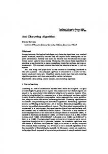
FIG. 1. 共Color online兲 Working of the PDB algorithm in the Zachary network. 共a兲 shows the initial vertices 共labeled with 2兲, which are seeds for the random walkers vertices labeled. 共b兲 shows the initial partition of the network into communities produced by the random walker stage. 共c兲 and 共d兲 show different partitions created by the modularity optimization process. The optimal partition, whose modularity is maximal, is shown in 共c兲.

based on modularity optimization usually have even more expensive search heuristics that allow a better exploration at the expense of efficiency. Our proposal was designed to focus on efficiency, as it can be seen in the heuristic decisions made by the algorithm. However, as we will show in the experiments section, this focus on efficiency does not necessarily imply a loss of quality of the clustering. A. Parallelization

To reduce even further the execution time of the algorithm its parallelization could be easily implemented. The stochastic process as defined in Eq. 共3兲 can be carried out in parallel by different computers or processors. To calculate the probability distribution of a given set of random walkers, only the transition probability matrix is required. Thus, the matrix G of dimension n ⫻ s could be split column by column into a set of smaller matrices of dimension n ⫻ ␵, where ␵ Ⰶ s. This would drastically reduce the cost of the stochastic process. Unfortunately, the modularity optimization step cannot be parallelized so easily. Thus, trivial parallelization would only affect the spectral analysis part of the algorithm. Although this part is the most expensive part in the algorithm O共ns兲, the modurality optimization O共s2兲 would still be executed sequentially. Therefore, the asymptotic cost of the PBD algorithm would still be O共n2兲. B. Working example with Zachary’s network

To illustrate our algorithm, we include an execution on the Zachary network 关34兴, which is a well-known data set in the literature of community extraction. In Fig. 1, we can find the network at the different stages of the execution of the

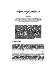
FIG. 2. 共Color online兲 Community structure of the Zachary network produced by the PDB algorithm. Circles and squares over the individuals denote to whom they align to after the karate club broke up. Those who aligned with the instructor are represented by circles, and those who aligned with the administrator are represented by squares.

algorithm. Figure 1共a兲 shows which vertices, labeled 2, are seeds of the random walkers, 16 in total. Thus, s is 16 compared to the original 34 vertices. In Table II, the relation between network size n and the number of random walkers s for a wide range of networks is shown. Figure 1共b兲 shows the initial partition of the networks produced by the random walker process, described in Eq. 共3兲. The initial 34 vertices are grouped into 13 groups. This partition has a modularity Q of 0.1547. From that point on the algorithm starts the modularity optimization stage governed by Eq. 共4兲. At each step, two of the remaining groups are joined according to Eq. 共4兲. Figures 1共c兲 and 1共d兲 show the network divided into four and two groups, respectively. The community structure of Zachary’s is better seen in Fig. 2. The maximum modularity is obtained by the partition in 4 communities, achieving Q = 0.3937. However, the original empirical work on the Zachary Karate Club 关34兴 found two communities: those aligned with the instructor and those aligned with the administrator. The division into two groups produced by the PBD algorithm produces a high modularity Q = 0.3718. Also, the two original communities found empirically correspond to the communities found by the algorithm with the exception of node 10, which is misclassified. It is evident that Fig. 2 is not a dendrogram over all the vertices of the network, but a dendrogram over the initial communities. As a consequence of the random walker process, the structure between vertices belonging to the same initial community remains unknown. However, this loss is negligible since the relevant high-level structure is not affected as can be seen in Fig. 2. III. EXPERIMENTS

In order to further analyze our algorithm, we chose a set of ten different networks of different sizes, ranging from 34 to 498 925 vertices. The networks modeled a wide spectrum of systems. There are social networks, such as the Zachary Karate Club 关34兴 and the social network of the Software Department 共LSI兲 at the Technical University of Catalonia

016107-4



关35兴; scientific collaboration networks, such as Cond-mat 关4兴 and the Erdös collaboration network 关36兴; citation networks, such as Scientometrics 关37兴; and affiliation network among Spanish top director boards 关38兴; a network of relations between words, such as WordNet 关39兴; metabolic networks, such as the C. Elegans 关40兴; a portion of the Web from the Notre Dame University data set 关1兴; and the last type of network was the movie collaboration 关41兴 network, again obtained from the Notre Dame University data set 关42兴. In all the networks we only worked with the biggest connex component, removing all multiple relations and self-reference edges. A. Comparing modularity

Table I summarizes the highest modularity achieved by Newman’s fast algorithm 共QN兲关14兴 and our algorithm 共QPBD兲. For eight out of the ten tested networks, the PBD algorithm produces a higher modularity, and the maximum difference in favor of the PBD algorithm is in the cond-mat network. Thus, in general, the PBD algorithm yields a slightly better modularity than the Newman’s fast algorithm. However, as mentioned in the Introduction, there exist in the literature other algorithms based on modularity optimization that also outperform the Newman’s fast algorithm 关14兴. In Table I, we also included the results obtained by the extremal optimization algorithm 共EO兲 by Duch and Arenas 关16兴. In this case the maximum modularity obtained by EO outperforms in two of three cases the modularity obtained using PDB, and in all the available cases it outperforms the modularity obtained using the Newman’s fast algorithm. However, the complexity of the algorithms that use elaborated search heuristics is superior to the complexity of both the Newman’s Fast algorithm and the PDB algorithm. For instance, EO’s complexity is O共n2 log2n兲. Thus, we can conclude that PDB has a good balance between efficiency and quality. B. Comparing the number of communities

Clustering, though, does not only depend on obtaining the partition that maximizes modularity. The number of communities—or groups—contained in the optimal partition is also very important. In Table I, the number of communities is denoted by gN, gEO, gPBD. We can clearly observe an order gEO ⬎ gN ⬎ gPBD. Provided that maximum modularity does not greatly differ between partitions, the huge differences in the number of communities obtained by the different algorithms are indeed striking and requires further study. Provided we assume that modularity Q is a good measure for community structure, we must take for granted that two partitions with similar modularity are equally accurate. Thinking otherwise would lead us to the conclusion that modularity is not a good measure. Finding a bogus partition that yielded higher modularity than a good partition would mean that modularity is not representative of the structure. Consequently, it could not be used as the fitness variable for the optimization. However we do not believe that this is the case. So, if we assume that modularity is a good measure, what happens when two partitions having very similar modularity

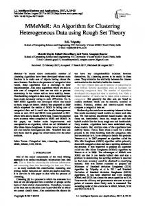
FIG. 3. 共Color online兲 Modularity Q over the execution of the algorithms for the cond-mat network. The PBD algorithm is shown as the solid line and the Newman’s fast algorithm 共N兲 as the dashed line. Note that the number of merge operations required for both algorithms is different 共PBD optimization stage starts with the partition given by the spectral analysis stage兲. PBD algorithm requires approximately the 22% of the merge operations performed by the N algorithm. Both the figure and the inset contain the very same information, but it is depicted in a different fashion to better illustrate the evolution of modularity. Note that the main figure is plotted in a log scale, and the time goes from right to left. This is done in order to magnify the last steps of the algorithms, which is when maximum modularity is found. We would like to remark that the number of remaining groups decreases over time, while the number of merge operations increases over time.

have a very different number of groups? A first approach would be to think that the partition with smaller number of groups is more general than the partition with the larger number of groups. Thus, partitions with smaller number of groups would be, in principle, more interesting for several reasons. 共i兲 They would provide a more general perspective on the underlying structure of the network, since they would be able to find a meaningful partition at a higher level of the structure. 共ii兲 A small number of groups would simplify the analysis of the obtained results. And 共iii兲, general or highorder partitions could always be reclustered to further analyze the structure of a particular group if a more detailed, fine-grained analysis was required. The opposite could not be done; otherwise, the algorithm would have detected the more general partition with higher modularity. Table I shows that the PBD algorithm yields more general partitions while having similar or better modularity. This effect is specially acute in large networks. One might conclude from the results of the experiments that both EO and N algorithms undergo an unnecessary over-specialization. For instance, let us we take the optimal partition of the cond-mat network. The PBD provides the highest modularity and the smallest number of partitions, which is 647, 324, and 44 using EO, N, and PBD algorithms, respectively. Figure 3 shows the evolution of Q in the cond-mat network using N and PDB algorithm. Note that the modularity

016107-5



FIG. 4. Behavior of the merge operation of the PBD 共above兲 and the N 共below兲 algorithms. For each merge operation the normalized ratio of the size of groups to be merged is calculated as rmo min共si,s j兲

= si+s j , where si and s j are the size of group i and j, respectively. The merge operation creates a new group z = i 艛 j of size sz = si + s j. The line corresponds to the evolution of modularity Q.

obtained by the N algorithm is very close to its maximum modularity when the number of remaining groups is in the range between 40 and 1000. Once the partition contains more than 1000 groups, it does not increase or decrease substantially until the number of groups in the partition reaches 40; at that point, modularity starts to decrease abruptly. This range of stable modularity contains a partition with 44 groups, which is the maximum modularity found by the PBD algorithm. This behavior is not observed in the evolution of modularity for the PBD algorithm, which keeps increasing modularity until it gets to the maximum and then it starts a quick descent. Being on a plateau where modularity is neither increasing or decreasing significatively might suggest that the search heuristic of the N algorithm could be stuck in a local suboptimal state. A more detailed study of the internal behavior of the N and PBD algorithms is described in Fig. 4, where the evolution of the normalized size of groups to be merged is depicted. Each merge operation joins group i and j in a new group z. The size of the two groups chosen by the algorithm min共si,s j兲

to be merged is expressed as rmo = si+s j . The ratio rmo has values in the range 共0 . . . 21 兴, when rmo is close to zero means that there is one group that is clearly bigger than its counterpart. When rmo = 21 both groups have the same size. It is easy to see how the N algorithm tends to join groups of very different size, whereas the PBD algorithm tends to do the opposite, i.e., it prefers groups of similar size. Consequently, the N algorithm produces at the very beginning groups of extremely large size by joining a single vertice to a very large group, when this group cannot accept more vertices a new group is started. This behavior is clearly observed at operation 6000, 10 000, and 15 000, approximately, creating three massive groups of 13 000 vertices and leaving the rest of groups composed mostly by individual vertices. This

might be the reason why the search heuristic fails to increase modularity in the plateau of Fig. 3. Approximately from operation 16 000 to 26 000, this behavior is not so evident, where groups of similar same size are often merged. However, the behavior that merges very dissimilar groups appears again between operations 26 000 and 27 000, overlapping the plateau of modularity. At this point, big groups cannot be merged obtaining a gain of modularity; therefore, the only possible option left to be explored by the search heuristic is to merge leftover groups of very few vertices into the existing big groups. As a consequence, the search heuristic gets stuck in a situation where changes of modularity are minimum and there is no escape from the suboptimal partition. The bias of the N algorithm toward creating very large groups has also been very recently reported by Danon et al. 关18兴. We can see how this behavior is not present in the PBD algorithm. The greedy search heuristic used by the PBD algorithm forces the worst group to be the one going to be merged, and this results in groups having similar sizes. By doing so, the search heuristic has many possible combinations to explore, avoiding getting trapped too early in a local suboptimum as it happened in the N algorithm. That is the reason why the PBD algorithm is able to find in the cond-mat network a higher modularity partition, which also has less groups. As for the EO algorithm, we could not carry out the same analysis, but it is plausible that the resulting large number of groups can be attributed to its divisive clustering strategy. In order to analyze with more detail the partitions yielded by the N and the PDB algorithms, the distance between the optimal partitions for the cond-mat network are calculated. Gustafsson et al. 关43兴 reviewed different distance measures to compare partitions of the same network. Since we want to look into the hypothesis that the partition yielded by the PDB 共PPBD兲 is more general than the partition yielded by N algorithm 共PN兲, we chose the mdiv measure, which is the minimum number of divisions to be applied to partitions A and B to obtain the partition C defined in 关44兴 as 兩A兩兩B兩

C = 艛艛共ai 艚 b j兲. i=1 j=1

共6兲

Partition C is the union of all possible intersections between the groups in A and B. We rename C as PN-PBD. The distance between partition PPBD and PN-PBD is 894, which is the number of divisions to be applied to PPBD in order to obtain PN-PBD. The distance between PN and PN-PBD is 614. Thus, the total distance is 1508, which is the sum of both distances. In order to have a baseline comparison for the distance between PPBD and PN, we created a random partition Prand with the same cardinality as PPBD. The random partition was replicated 30 times and so was the measurement; the average distance between PN and Prand was 7166.7 with a standard deviation of 33.65. C. Comparing efficiency

After comparing the quality of the clustering produced by the PBD algorithm, we must turn our attention toward its performance. As we already mentioned, all design decisions

016107-6



FIG. 5. 共Color online兲 Comparison between the efficiency in CPU time 共in seconds兲 for ten networks of different sizes. The solid circles show the results for the Newman’s fast algorithm. The results of the PBD algorithm are represented by solid squares.

were biased toward improving the efficiency so that the algorithm could cope with medium and large networks, which other algorithms cannot handle in reasonable time. Table II summarizes the run time 共CPU time兲 of our algorithm compared to the Newman’s fast algorithm, which is the reference algorithm due to its efficiency. We are perfectly aware of the problems related to comparison of algorithms based on run time instead of only considering their complexity. In order allow a fair comparison between both algorithms, we implemented them from scratch optimizing them to the best of our abilities. Needless to say, the runs were executed on the same desktop computer 共Pentium 4, 3 GHz兲 exclusively dedicated to the experiment. Table II shows that PBD is much faster than the Newman’s fast algorithm for networks bigger than 1000 vertices. Conversely, the PBD algorithm is slower than the N algorithm for small networks. This is because the two sequential processes—spectral analysis and modularity optimization—that take place in the PBD algorithm. The difference in execution time heavily depends on the number of random walkers 共sPBD兲 required for the first stage of the PDB algorithm. The smaller the ratio between network size and the number of random walkers, the faster the PDB algorithm is. Figure 5 graphically shows the relation between network size and the running time of both algorithms already seen in Table II. The PDB algorithm clearly outperforms the Newman’s fast algorithm, often by one order of magnitude. However, the asymptotic quadratic behavior of both algorithms is evident, which lead us to think that our algorithm cannot scale to very large networks of millions of nodes. Resorting to parallelization would allow us to analyze networks of a few million nodes in an acceptable time; however, the PDB will undoubtedly become too slow for very large networks. Nonetheless, it allows to shift the network size threshold far

FIG. 6. 共Color online兲 Fraction of vertices correctly classified using computer-generated networks. The circles show the result of the Girvan-Newman algorithm 共GN兲. The squares show the results of the PBD algorithm. Each point is an average over 50 networks.

enough to be useful for medium and large networks. Reduction of approximately one order of magnitude allows one to shift from minutes to seconds or from hours to minutes. For instance, the clustering of the largest network we had access to was reduced from ⬃9 h to just one. Computer-generated networks

To conclude, we include experiments carried out with the computer-generated networks first proposed by Girvan and Newman 关11兴, which have become a common testbed in the field. Those networks are constructed with 128 nodes divided into four groups of the same size. For each node, eight edges are deployed. With probability Pin the edge is connected to a node that belongs to the same group chosen at random. Otherwise, the edge is connected to a node that does not belong to the same group. Thus, the average degree of a node is 16. Accordingly to the nomenclature of Girvan-Newman, we will use zout which is the number of intercommunity edges per node. It is important to note that for zout = 12, the network is totally random; that is, without community structure. Another important value for zout is 8, since it marks the boundary between having more intercommunity than intracommunity edges. The quality measurement is the fraction of vertices that are correctly classified, explained in more detail in 关14兴. In Fig. 6, we can see the results obtained by our algorithm compared to the results yield by the Girvan-Newman 共GN兲 algorithm based on edge betweenness 关11兴. We decided to use the GN algorithm instead of the Newman’s fast algorithm since it obtains slightly better results, and it is the reference algorithm for this particular experiment 关11兴. Although the results of GN outperform those obtained by the N algorithm, it is not a suitable option for medium and large networks due to its complexity; that is O共n3兲. The GN algorithm correctly detects the communities until values of zout = 6 are reached. From this point on, the quality

016107-7



of the communities decreases very quickly. On the other hand, the PBD algorithm detects the communities very well up to values of zout = 7; from that point on the performance starts to decay, although the pace is more steady than in the GN case. As already mentioned, other algorithms based on modularity optimization perform much better in the computer-generated networks example. For instance, Duch and Arenas extremal optimization algorithm 关16兴 starts to decline at zout = 8. However, its increase on clustering quality is done at the expense of efficiency. Thus, it is unadvisable in the case of large networks. IV. CONCLUSIONS

In this paper, we have presented an algorithm to extract community structure from networks by using a combination of different existing methods. First, the algorithm uses spectral analysis via the multiple random walker process to reduce the dimensionality of the network by creating the initial partition of the network into communities. Then, a modularity optimization process with a extremely greedy search heuristic is applied to extract the underlying structure of the network. Experiments show that our algorithm outperforms the Newman’s fast algorithm both in clustering quality and efficiency. The Newman’s fast algorithm is the reference algorithm in terms of efficiency, and while asymptotically both algorithms are O共n2兲, the PDB algorithm is always faster in computation time for medium and large networks, as it has been shown in the experiments.

关1兴 R. Albert, H. Jeong, and A.-L. Barabási, Nature 共London兲 401, 130 共1999兲. 关2兴 F. Liljeros, C. Edling, L. Amaral, H. Stanley, and Y. Aberg, Nature 共London兲 411, 907 共2001兲. 关3兴 B. A.-L., H. Jeong, E. Ravasz, Z. Néda, A. Schubert, and T. Vicsek, e-print cond-mat/0104162. 关4兴 M. Newman, Phys. Rev. E 64, 016131 共2000兲. 关5兴 H. Jeong, S. Mason, Z. Oltvai, and A.-L. Barabási, Nature 共London兲 411, 41 共2001兲. 关6兴 R. Albert, H. Jeong, and A.-L. Barabási, Nature 共London兲 406, 378 共2000兲. 关7兴 W. Aiello, F. Chung, and L. Lu, in Proceedings of the 32nd ACM Symposium on the Theory of Computing, edited by F. Yao 共ACM, New York, 2000兲, p. 171. 关8兴 R. Albert and A.-L. Barabási, Rev. Mod. Phys. 74, 47 共2002兲. 关9兴 M. Newman, SIREV 45, 167 共2003兲. 关10兴 D. Watts and S. Strogatz, Nature 共London兲 393, 440 共1998兲. 关11兴 M. Girvan and M. Newman, Proc. Natl. Acad. Sci. U.S.A. 99, 7821 共2002兲. 关12兴 R. Kannan, S. Vampala, and A. Vetta, in Foundations of Computer Science 共IEEE Computer Society, Redondo Beach, CA 2000兲, p. 367. 关13兴 M. Newman and M. Girvan, Phys. Rev. E 69, 026113 共2004兲. 关14兴 M. Newman, Phys. Rev. E 69, 066113 共2004兲. 关15兴 R. Guimerà and L. Amaral, Nature 共London兲 433, 895 共2005兲.

The reason behind this is the reduction of dimensionality provided by the random walker process, such that the cost of the PBD can be expressed as O共ns兲 where s Ⰶ n. Furthermore, experiments also show that the PDB retrieves more general community structure than other algorithms. The number of existing communities in the partition with maximum modularity is notably smaller in the case of the PBD. This fact leads us to think that other algorithms tend to unnecessarily over-specialize their clustering. In summary, the presented algorithm is an interesting choice when analyzing medium and large networks. The structure of large networks can be found in reasonable time, from seconds for a network of 27 000 vertices to less than one hour for a network of 500 000 vertices. The gain in efficiency does not come with a loss in the quality of the clustering as the maximum modularity obtained by the algorithm is comparable to the reference algorithms in the literature. ACKNOWLEDGMENTS

The authors would like to thank Jordi Duch and Alex Arenas for helpful comments and for providing us with the binary of their EO algorithm 关16兴. We also thank Mark Newman, Fabrizio Ferraro, and Mariano Belinsky for providing some of the data sets used in the experiment. This is also extended to those researchers that compiled and made public the remaining data sets used in the experiments. This research was supported by the Spanish Government Grant No. CICYT-TIC2003-1120-C03-02.

关16兴 J. Duch and A. Arenas, Phys. Rev. E 72, 027104 共2005兲. 关17兴 M. Newman, e-print physics/0602124. 关18兴 L. Danon, A. Díaz-Guilera, and A. Arenas, e-print physics/ 0601144. 关19兴 S. Wasserman and K. Faust, Social Network Analysis: Methods and Applications 共Cambridge University Press, Cambridge, England, 1994兲. 关20兴 D. Gibson, J. Kleinberg, and P. Raghavan, in Proceedings of the ACM Symposium on Hypertext and Hypermedia 共ACM Press, New York, 1998兲, p. 225. 关21兴 R. Kumar, P. Raghavan, S. Rajagopalan, and A. Tomkins, in Proceedings of the 8th World Wide Web Conference 共Elsevier Science, Essex, UK, 1999兲, p. 403. 关22兴 C. Borgs, J. Chayes, M. Mahdian, and A. Saberi, in Proceedings of KDD 共ACM Press, New York, 2004兲, p. 783. 关23兴 D. Bu, Y. Zhao, L. Cai, H. Xue, X. Zhu, H. Lu, J. Zhang, S. Sun, L. Ling, N. Zhang et al., Nucleic Acids Res. 91, 2443 共2003兲. 关24兴 H. D. Simon, Comput. Sci. Eng. 2, 135 共1991兲. 关25兴 L. Page, S. Brin, R. Motowani, and T. Winograd, Tech. Report No. 1997-0072, Stanford Digital Library Working Paper 共1997兲. 关26兴 J. Kleinberg, Tech. Report No. RJ 10076, IBM 共1997兲. 关27兴 G. Flake, R. Tarjan, and K. Tsioutsiouliklis, Internet Mathematics 1, 385 共2003兲.

016107-8


CLUSTERING ALGORITHM FOR DETERMINING¼ 关28兴 D. Harel and Y. Koren, Lect. Notes Comput. Sci. 2245, 18 共2001兲. 关29兴 U. Brandes, M. Gaertler, and D. Wagner, Lect. Notes Comput. Sci. 2832, 568 共2003兲. 关30兴 A. Jain and R. Dubes, Algorithms for Clustering Data 共Prentice-Hall, Englewood Cliffs, NJ, 1988兲. 关31兴 A. Jain, M. Murty, and P. Flynn, ACM Comput. Surv. 31 共1999兲. 关32兴 E. Forgy, Biometrics 21, 768 共1965兲. 关33兴 P. Bradley and U. Fayyad, in Proceedings of the 15th Intl. Conf. on Machine Learning 共Morgan Kaufmann, New York, 1998兲, p. 91. 关34兴 W. W. Zachary, J. Anthropol. Res. 33 共1977兲. 关35兴 R. Sangüesa and J. Pujol, Knowledge Management and Organizational Memories 共Kluwer, Dordrecht, 2002兲. 关36兴 Erdös Number Project. The network contains scientists with Erdös number less than or equal to 2 up to year 2002. http:// www.oakland.edu/enp/thedata.html 关37兴 Network from Garfield’s collection of citation networks. Avail-

关38兴

关39兴关40兴关41兴

关42兴关43兴关44兴

016107-9

able at http://www.garfield.library.upenn.edu/histcomp/ index.html Data provided by Fabrizio Ferraro, from the project Small Worlds of Corporate Networks at IESE Business School, University of Navarra Network obtained from the Pajek Network dataset. Available at http://vlado.fmf.uni-lj.si/pub/networks/data/ H. Jeong, B. Tombor, R. Albert, Z. Oltvai, and A.-L. Barabási, Nature 共London兲 407, 651 共2000兲. This network is a bipartite network 共two-mode兲. Consequently, vertices have different roles and thus the structure extracted by the algorithms might be biased. We did not transform it to a one-mode network to maintain the maximum of vertices. Thus, the results on this network are only relevant when speaking about the algorithm’s efficiency. A.-L. Barabási and R. Albert, Science 286, 509 共1999兲. M. Gustafsson, M. Hörnquist, and A. Lombardi, Physica A 共to be published兲. D. Gusfield, Inf. Process. Lett. 3, 159 共2002兲.