Via Madonna delle Carceri, 62032 Camerino (MC), Italy. (Received 26 May 1995). L-edge extended x-ray-absorption fine structure (EXAFS) spectra of solid and ...
PHYSICAL REVIEW B
VOLUME 53, NUMBER 10
1 MARCH 1996-II
Multiple-edge EXAFS refinement: Short-range structure in liquid and crystalline Sn Andrea Di Cicco Dipartimento di Matematica e Fisica, Universita` degli Studi di Camerino, Unita` di Ricerca INFM, Via Madonna delle Carceri, 62032 Camerino (MC), Italy ~Received 26 May 1995! L-edge extended x-ray-absorption fine structure ~EXAFS! spectra of solid and liquid tin have been collected by using synchrotron radiation. Information on local structure has been obtained by simultaneous analysis of Sn L 3 - , L 2 - , and L 1 -edge EXAFS spectra by using an original data-analysis scheme based on the ab initio multiple-scattering GNXAS method. The use of the three edges allowed the extension of the energy range of the useful data increasing the accuracy of the derived structural parameters. Details of the multiple-edge data-analysis methodology are provided. The general interest of the method for multiple-edge structural studies of monatomic and multiatomic systems is discussed. A very good agreement with diffraction data is found for crystalline Sn. The first-neighbor distribution is studied as a function of temperature. Statistical errors on the structural parameters are provided. The model pair distribution function g(r) obtained by x-ray-diffraction data is refined in liquid Sn at T5245 °C. The EXAFS structural signal is shown to be very sensitive to the short-range correlations. The foot of the first peak of the g(r) is found to be steeper and the mean distance is found slightly shorter than previously indicated. Error bars on the g(r), due to random errors in the EXAFS data, are also shown. The signature of a three-body signal assigned to short-range covalent tetrahedral configurations is evidenced.
I. INTRODUCTION
Quite recently, several advances in x-ray-absorption fine structure ~XAFS! data analysis have greatly improved the accuracy of the structural information obtained from XAFS experimental data. Major efforts have been devoted to the development of ab initio data-analysis methods based on spherical-wave multiple-scattering codes.1–3 In particular, the GNXAS method1,4,5 has been used on several molecular, crystalline, and disordered systems always giving very accurate results. Typical statistical errors were found to be in the 0.001 Å range for first-shell average bond distance depending on the quality of the experimental data. This method is based on a n-body decomposition of the x-ray-absorption cross section and presents several advantages: ~i! the configurational average of the multiplescattering terms is properly accounted for providing a tool to investigate three-body correlations in ordered and disordered systems; ~ii! the raw absorption data are used without any filtering allowing to account for the presence of manyelectron excitations and to perform a full statistical analysis of the results. An updated list of references can be found in Refs. 4 and 5. It is worth mentioning that this approach has been also successfully used to investigate three-body correlations in disordered systems where covalent or nearly covalent bonds are present.6 – 8 In this work I shall examine the case of the L-edge XAFS of crystalline and liquid tin ~l-Sn! as a function of temperature. A few previous XAFS studies dealt with combined L edge data analysis, and made use mainly of very approximate relations between the L 3 , L 2 oscillations and the L 1 one. An extensive literature and a discussion on problems and methods to perform L-edge data analysis is contained in 0163-1829/96/53~10!/6174~12!/$10.00
53
Ref. 9. Here, the L-edge data analysis is successfully performed using a novel approach based on the abovementioned GNXAS method. A multiple-edge XAFS refinement is implemented in order to increase the accuracy and consistency of the structural results in the present Sn L-edge case where the available energy range for each edge is quite limited. In this way, a few structural parameters are used to fit simultaneously the three L edges. It has to be stressed that, due to the narrow energy range available, the Fourier filtering technique is not useful in this case. Moreover, the present scheme for data analysis can be easily extended to other multiedge studies of monatomic and multiatomic systems and deserves general interest. In the present study the crystalline b -Sn spectra are taken as reference for the successive study of liquid tin. Local structure information derived from XAFS data analysis is compared with the known crystallographic and vibrational data. Of course, the investigation presented in this work is of particular interest for the study of the liquid structure, for which the main information is currently represented by the structure factor S(k) measured by diffraction. Many x-ray-10–12 and neutron13–15 diffraction investigations of l-Sn have been carried out. Although quite scattered, diffraction data just above the melting point always show the characteristic hump after the first S(k) peak. This feature is generally present in those elements ~Ga, Bi for example! whose crystal structure shows a low degree of symmetry. Recently, reverse Monte Carlo ~RMC! techniques have been used to derive realistic structural models in l-Sn and evidence for tetrahedral bonding was found.16 In view of the existing differences in the diffraction data and of the high sensitivity of XAFS to the very short-range local two-body and three-body distributions, the application of XAFS for the refinement of the local 6174
© 1996 The American Physical Society
53
MULTIPLE-EDGE EXAFS REFINEMENT: SHORT-RANGE . . .
FIG. 1. Design of low-melting point metal samples ~Sn in the present work! suitable for transmission XAFS measurements in the liquid phase.
structure in l-Sn is certainly very interesting. Previously, only a very short report of a Sn K-edge XAFS study on liquid tin has been published.17 Here, the use of a large number of energy points associated with the L 3 , L 2 , and L 1 XAFS has allowed an accurate refinement of the local g(r) of l-Sn. The paper is organized as follows: in Sec. II a description of the experimental details concerning measurements and preparation of samples is reported; in Sec. III the multiedge data-analysis scheme is illustrated; in Sec. IV the multiedge b -Sn data analysis is presented; results on l-Sn are reported in Sec. V along with a detailed comparison with previous diffraction results; Sec. VI is devoted to the conclusions. II. EXPERIMENTAL DETAILS
X-ray-absorption measurements near the Sn L 3 , L 2 , and L 1 edges were performed in transmission mode at the storage ring ADONE ~Laboratori Nazionali di Frascati, INFN! working at 1.5 GeV with a typical current of 50 mA during dedicated beam time on the PULS ~Progetto per l’Utilizzazione della Luce di Sincrotrone! x-ray beam line, using a Si ~111! channel-cut monochromator and a 1 mm slit. Measurements were carried out at several temperatures below and above the melting points using a furnace18 working under vacuum conditions. A crucial problem to be solved is the establishment of a suitable sample preparation technique. In fact, homogeneous films of about 2 m m thickness have to be used in order to obtain the best signal-to-noise ratio in the selected photon energy range ~around 4 keV!. Moreover, the sample has to be designed in order to be able to resist to several thermal cycles below and above the melting point. For this purpose, the following preparation technique was used ~see Fig. 1!. ~i! A suitable low x-ray-absorbing substrate was chosen. For this purpose standard Goodfellow 50350 mm graphite foils of 100 m m thinness were found to be both a low-cost and a high lifetime solution. ~ii! A SiO ~Aldrich chemical co. 99.99%! film of about
6175
2000 Å thickness was deposited using a Ta crucible ~deposition rate of about 20 Å/s! over the graphite substrate. Pressure inside the deposition chamber was about 5310 25 Pa. ~iii! A metal film ~Sn Heraus 99.9999%! of suitable thickness has been deposited using a W crucible ~deposition rate was about 1 Å/s! on the composite graphite1SiO foil through a 5315 mm mask. Pressure was maintained below 1 310 24 Pa. ~iv! A second layer of SiO ~thickness of about 4000 Å! was deposited on the whole surface of previously prepared composite substrates @steps ~i!-~iii!#. The depositions were carried out at the University of Camerino using a Leybold-Heraus UNIVEX 300 evaporation apparatus equipped with an INFICON XTM thickness and rate of deposition monitor. The technique illustrated at the points ~i!-~iv! allows one to prepare samples where the metal foil is folded between two thin layers of an inert substance. In this case the silicon oxide film was not found to react with the metal in the temperature range under consideration (T,300 °C!. At the same time, the sample does not change shape as a consequence of melting and can be safely measured in the liquid state. Of course, this sample preparation technique works for low-melting-point metals which do not react with SiO or graphite. For example, a similar sample preparation technique was used in a pioneering study on liquid zinc.19 For high-melting-point or highly reactive substances different sample preparation methods have to be used.20 The samples were measured at several temperatures above and below the melting point (T m 5231.9 °C!. Fast XANES ~x-ray-absorption near-edge structure! spectra were recorded during the thermal cycles in order to monitor the solid-liquid transition. XAFS spectra in an extended energy range including all of the three L edges have been also recorded at selected temperatures using longer integration times ~typically 10 s for each energy point!. Neither oxidation nor loss of tin sample took place during the thermal cycles. The final room temperature spectra were checked to be equal to the initial one within the experimental noise. In Fig. 2 the L 3 , L 2 , and L 1 x-ray-absorption coefficient of liquid tin at T5245 °C is shown. In spite of the relatively large absorbance of the graphite foil at these energies, the signal-to-noise ratio is found to be quite good, around 10 3 ~see next section!. In Fig. 3 the L 3 XANES spectra at different temperatures below and above ~upper curve! the melting point are shown. The change in the local structure occurring at the melting point is clearly reflected in the corresponding change of the XAFS pattern in the liquid phase. III. MULTIEDGE ab initio DATA ANALYSIS
In this paper the first attempt of a multiedge study using the above-mentioned ab initio MS GNXAS method is presented. The method, as it has been shown in detail in previous publications,1,4,5 is based on a direct comparison of a model theoretical signal containing the relevant two-atom and three-atom MS terms ( g (2) and g (3) , see Refs. 1, 4, and 5! associated with selected atomic configurations with the raw experimental data ~absorption coefficient a expt). The model signal a mod , calculated using a model structure, is then refined by minimizing a standard x 2 -like residual function:
ANDREA DI CICCO
6176
53 M
a mod~ E ! 5 (
i51
i! ~ E2E ~0i ! !# # @ J i s ~0i !~ E !@ 11S 20 ~ i !x ~mod
1 a bkg~ E ! 1 a exc~ E ! .
FIG. 2. Raw L 3 -, L 2 -, and L 1 -edge absorption data of liquid tin at T5245 °C. N
R~ $l% !5
(
i51
@ a expt~ E i ! 2 a mod~ E i ;l 1 ,l 2 , . . . ,l p !# 2
s 2i
. ~1!
In Eq. ~1! the index i runs over the number N of experimental energy points E i , $ l % 5(l 1 ,l 2 , . . . ,l p ) are the p parameters to be refined and s 2i is the variance associated with the a expt2 a mod random variable. The model absorption signal associated with a set of M different atomic edges is given by
FIG. 3. Near-edge Sn L 3 spectra at different temperatures in the solid and liquid phases. While the three (a), (b), and (c) spectra recorded below the melting point preserve the same shape, the liquid spectrum ~top! shows a clearly different pattern.
~2!
In Eq. ~2! E is the photon energy, x (i) mod is the actual XAFS signal containing the structural information related to the selected ith edge ~sum of integrals of the g (n) terms, see Refs. 1 and 4 – 6!, s (i) 0 (E) is a step function accounting for the atomic cross section of the absorption channel of interest. Above the selected edge s (i) 0 (E) is a decreasing smooth function of the energy and can be modeled using a hydrogenic functions or the McMaster tables. The background a bkg(E) is modeled as a smooth polynomial spline accounting for the preedge and postedge contributions of all of the absorption channels opened at lower energies. a exc(E) is a contribution in the postedge region accounting for possible multielectron excitation channels for which several evidence can be found in the literature ~see Ref. 21 and references therein!. The energy E (i) 0 defines the relation between the theoretical energy scale associated with the x (i) mod signals and the photon energy scale E. Usually the E (i) 0 value falls a few eV above the corresponding absorption threshold. and J i are both factors defining the intensity of the S 2(i) 0 is a constant reduction factor accounting model signal. S 2(i) 0 for effective many-body correction to the one-electron cross section. The scaling factor J i accounts for the actual density of the photoabsorber atoms. Due to the intrinsic uncertainty in the threshold shape of s (i) 0 (E) and to the inclusion of the contribution of possible many-body channels into the absorption cross section, the J i can be determined with a relative large relative error bar ~around 1022 ). The uncertainty on J i reflects naturally on S 2(i) and therefore this last parameter 0 acts as a phenomenological correction accounting for both many-body effects and uncertainty in the jump normalization. In order to compare a mod with the experimental data, the model spectrum is also convoluted with the energy resolution function of the monochromator. Other broadening effects due to photoelectron mean-free-path and core-hole lifetime ~different for each edge i! are included ab initio in the complex effective potential used to calculate x (i) mod . The use of Eq. ~1! allows one to perform a full statistical analysis of the structural results. In particular, it is possible to ¯ ,l ¯ ¯ l% 5(l obtain best-fit values $ l % 5 $ ¯ 1 2 , . . . ,lp ) along with their statistical errors including correlation among different parameters. This problem is treated in previous publications and I will refer to them for all the details.4,5 As mentioned in the Introduction, typical standard deviations in the 0.001– 0.01 Å range for first-neighbor bond distances have been found. There are several advantages in using the integrated multiedge approach presented in this paper: in fact, ~i! the increasing number of useful experimental points always allows a more accurate extraction of the structural parameters; moreover ~ii! in cases where a narrow energy range is available and XAFS signals are overlapping, as in the present Sn L-edge case, a robust estimate of the structural parameters is still possible; finally ~iii! for multiatomic systems consistent partial distribution functions can be easily extracted.
53
6177
MULTIPLE-EDGE EXAFS REFINEMENT: SHORT-RANGE . . .
FIG. 4. Estimated standard deviation of the Sn L 3 spectrum of Fig. 2. The dashed curve is the standard deviation function derived using Eq. ~3!.
Of course, experimental spectra should have signal-tonoise ratios of the same magnitude in order to take full advantage of the multiedge technique. In any case, the proper weight of different spectra contributing to the residual function is accounted for by the variance function s 2i which will be clearly larger in case of noisy spectra. Therefore, it is important to discuss the criteria for the estimate of the variance s 2i associated to each point of the random variable a expt2 a mod . In the following, the presence of systematic errors in the experimental measurements is not considered. The first contribution to the variance is due to the statistical noise s 2i(expt) of the experimental measurement a expt(E i ). Depending on the experimental conditions, typical values for s 2i(expt) are in the 1025 –1028 range. As a first approximation, s 2i(expt) can be considered a constant throughout a single XAFS scan. However, the actual behavior of the s 2i(expt) depends on the number of counts associated to the ith energy point. A simple way to estimate the variance of the data s 2i(expt) is to model the absorption coefficient over a selected number of energy points with polynomial functions. This works when the absorption coefficient is sampled using reasonable energy steps and in presence of a smooth XAFS signal. As an example, in Fig. 4 the s 2i(expt) pattern estimated using a seventh-order polynomial best fit over 50 experimental L-edge XAFS energy points ~l-Sn! is reported. The s 2i(expt) function appears to be slightly energy dependent, as expected looking at the variation in the number of counts in different regions of the a expt signal and considering the presence of small glitches. The largely increased variance near the edge ~dots! is due to the decreased number of counts but also to the presence of the white line and large XAFS oscillations which are not correctly reproduced by the model function. The increase of the variance in the edge region
results therefore overestimated and will not be considered. Generally speaking, the pattern of the s 2i(expt) function depends on the experiment itself, i.e., on the way of collecting experimental data. For example, for measurements in transmission mode the variance s 2i(expt) can increase in the nearedge region due to the decrease in the transmitted flux of photons, while using fluorescence detection the situation is reversed. Moreover, the actual energy dependence of the incoming flux I o can be considered, when important. In the present Sn L-edge case the increased flux at higher energies, due to both the synchrotron radiation energy pattern and to the decreased absorption of the windows and of the graphite foil, leads to a slight decrease of the variance in the L 1 spectrum. Furthermore, if increased acquisition times are used as a function of the wave-vector value k, it is clear that a smaller variance should be associated to points at higher energies. An increased statistics is sometimes used in combination with an energy-dependent mesh of energy points and therefore a few points with smaller variances are collected at high energies. In these cases, it is recommended to include an appropriate weighting accounting for the lower statistical error of the points in the higher-energy region. A second source of error contributing to the variance is due to the model signal a mod , where possible uncertainties come from the phase-shift calculation and modeling of the potentials, from intrinsic limitations of the underlying theory ~for example, the ‘‘one-electron’’ approximation! and from the lack of inclusion of specific multiple-scattering signals. These modeling problems can increase the variance s 2i in Eq. ~1!. In fact, as the a mod and a expt functions are statistically independent, it is possible to write: s 2i 5 s 2i(expt) 1 s 2i(mod) . The present status of the theory does not allow a precise estimate of the s 2i(mod) in the general case. However, the use of the muffin-tin approximation has been proven to be very reliable in the high-energy regime (k.4 Å 21 ). Non-muffintin corrections and self-consistent potentials are generally used to investigate the near-edge region. Moreover, the convergence properties of the MS expansions allows a very accurate modeling of the structural x (k) term at high energies, when only a few g or x n signals are used. The indetermination on the intrinsic E 0 value is another source of error contributing to s 2i(mod) . The effect of a variation of E 0 is obviously more important at lower k (k; AE2E 0 ) values @ D x (k);DE 0 /2k#. These arguments indicate that the highenergy region of the absorption coefficient can be more accurately modeled. All of the above-mentioned sources of uncertainty have to be considered in the construction of a realistic s 2i . In principle, quite complex functions accounting for the various effects could be used for the estimate of s 2i . However, the use of a simple power law accounting for all of the different error sources has been often preferred. The following power-law expression
s 2i 5 s ~2expt!
p k max
k ip
~3!
guarantees the fulfillment of the lower limit of s 2i at high energies. In fact, the statistical noise of the experimental
6178
53
ANDREA DI CICCO
measurement ( s 2i(expt) ) is the lower limit for the variance. In Eq. ~3! a constant value ( s 2(expt) ) instead of the actual 2 s i(expt! is used, leaving the energy dependence only to the p weighting factor k 2 i . k max is the upper wave-vector value in the XAFS spectrum under consideration. It has to be remarked that the use of a power-law weighting of the data is common practice in XAFS data analysis. In fact, k p (p5123) weighting of XAFS data was originally introduced in the standard Fourier filtering data-analysis techniques in order to compensate the amplitude decrease of the XAFS signal at high k values. In the present context, the necessity of an increased weight ~lower variance! at higher energies is due to the reasons outlined above. In Fig. 4 the dashed curve is the standard deviation s i calculated for the l-Sn spectrum using Eq. ~3! with p52. s 2(expt) has been obtained as an average on the s 2i(expt) values ~the near-edge overestimated values of s 2i(expt) are excluded!, neglecting the slight differences between the L 1 , L 2 , and L 3 s 2(expt) average variances. The s i functions obtained in this way have been used both in the b -Sn and in the l-Sn cases for calculating the residual function. IV. CRYSTALLINE TIN: RESULTS AND DISCUSSION
In this section the MS data analysis of the L-edge data of (L i ) b -Sn ~white tin! is described. The model x mod (k) (i51,3! signals associated with all of the L edges have been calculated using two-body ( g (2) ) and three-body ( g (3) ) terms associated with local two-atom and three-atom configurations limited within 6 Å. Complex and energy-dependent self-energies @HedinLundqvist ~Ref. 22!# have been used in the construction of the nonoverlapping muffin-tin potentials ~tangent muffin-tin spheres have been chosen!.23 The proper core-hole lifetimes have been also included in the imaginary part of the potential. In Table I the average coordinates and degeneracy of the b -Sn two-atom and three-atom configurations found within 6 Å as derived from the tabulated lattice parameters ~Ref. 24 and references therein! are reported. As reported in Table I, there are six irreducible two-atom configurations in b -Sn. The g (2) signals associated with these configurations have been calculated for all of the L-edges. While the two-atom configurations are simply defined by using the interatomic distance, the three-atom ones need at least three coordinates. The natural choice is given by the two shortest interatomic distances R 1 , R 2 and the angle in between u . In b -Sn, there are five three-atom configurations showing a half-perimeter length within the 6 Å cutoff. In this monatomic system the photoabsorbing atom can be in any position of these three-atom configurations. The total g (3) signal associated with a certain three-atom configuration is given by the sum of the signals obtained by changing the position of the photoabsorber. Thus, the photoabsorber position ~pos.! is an additional information given for the threeatom configurations. The individual degeneracy is given by the number of three-atom configurations per atom found in the structure. The main frequencies (R path) of the corresponding XAFS
TABLE I. Pair and triplet configurations in the b -Sn structure. The distances are reported in Å, the angles are in degrees. The degeneracy ~Deg.! is specified for each configuration. The photoabsorber position for the triplet configurations is also specified ~Pos.!. Position 1 corresponds to the vertex between the two short bonds, position 2 is at the end of the first bond ~with length R 1 ) and position 3 is at the end of the second bond. Peak Two-atom 1 2 3 4 5 6
R1
R2
u ~°!
configurations 3.022 3.181 3.768 4.420 4.931 5.832
Deg.
Pos.
4 2 4 8 4 4
Three-atom configurations 1 3.022 3.181
74.74
2
3.022
3.022
93.97
3
3.022
3.181
105.26
4
3.022
3.768
80.41
5
3.022
3.022
149.49
4 4 4 4 8 4 4 4 8 8 8 2 4
R path 3.022 3.181 3.768 4.420 4.931 5.832
1 2 3 1 2 1 2 3 1 2 3 1 2
4.986 4.986 4.986 5.232 5.232 5.567 5.567 5.567 5.605 5.605 5.605 5.938 5.938
g signals are also given in Table I. For the g (2) two-atom signals R path simply corresponds to the interatomic distance while for the three-atom g (3) signals it corresponds to the half-perimeter of the triangular configuration. The configurations are numbered according to their R path typical length. There is an obvious hierarchical connection between the two-atom and three-atom configurations. The three R 1 , R 2 , and u average parameters automatically define the third interatomic distance (R 3 ) of the triangular configuration. In particular, the third, fourth, and fifth interatomic distances are related to the first, second ~fourth!, and third triangular configurations, respectively. The sixth interatomic distance is related to the fifth triangular configuration. Therefore the two-atom g (2) signals beyond the second shell can be calculated using the corresponding three-atom coordinates avoiding the introduction of further structural parameters. In the following, a single effective MS signal h (3) including both the g (2) and the g (3) contributions will be used for the shells beyond the second one using the same three-atom coordinates both for the two-atom and the three-atom terms. The configurational average of the g signals, related to the thermal motion and/or to the static disorder, is finally performed in order to calculate the x mod(k) signals to be inserted in Eq. ~2!. In the following we will refer to the bond-length distribution associated with a selected interatomic distance as a ‘‘peak’’ of the two-atom distribution function. Correspondingly, the distribution of the triangular coordinates associated with a particular triangular arrange-
53
MULTIPLE-EDGE EXAFS REFINEMENT: SHORT-RANGE . . .
FIG. 5. Best-fit MS signals for the Sn L 3 , L 2 , and L 1 XAFS k x (k) spectra ~left, middle, and right panels, respectively! recorded at room temperature ~22 °C!. The overall agreement between calculated and measured spectra is excellent. The dashed curves are the extensions of the XAFS signal related to the previous edges. Notice the large amplitude difference between the L 1 and L 3 (L 2 ) XAFS spectra.
ment is a ‘‘peak’’ of the three-body distribution. For crystalline systems at moderate temperatures Gaussian models for the peaks of the two-body and three-body distribution functions are accurate enough to account for thermal vibrations. There are specific formulas accounting for the thermal and configurational average of two-atom, three-atom, or n-atom MS g signals.25,1,5 Moreover, several different approximations for the shape of the distribution function peaks can be used. For hot crystals, the harmonic approximation fails and it is necessary to account for the asymmetry of the peaks. Both the cumulant expansion or suitable distribution curves can be used in these cases. The overcoming of the Gaussian approximation is particularly important in the case of highly disordered and liquid systems ~see next section!. In the b -Sn case we have used an Euler G function to describe the first-neighbor distribution.26,27 The distribution depends on three parameters: the usual R and s 2 ~interatomic mean distance and variance!, and the adimensional skewness parameter b 5K 3 / s 3 , where K 3 is the third cumulant of the distribution. The introduction of a slight asymmetry has been found important to model the first-neighbor distribution in this low-melting point element. In Fig. 5 the best-fit MS g signals for the Sn L 3 , L 2 , and L 1 XAFS k x (k) spectra ~left, middle, and right panels, respectively! recorded at room temperature ~22 °C! are presented. From the top to the bottom the g (2) signals associated with the first two peaks of the two-atom distribution ~first and second shell! and the h (3) ones related to the first three three-atom configurations are reported. The h (3) signals contain both the proper three-atom term g (3) and the two-atom one ( g (2) ) associated with the longer interatomic distance of the triangle ~third, fourth, and fifth shell in this case!. Notice the remarkable amplitude difference between the L 1 and the L 3 (L 2 ) signals.
6179
FIG. 6. Fourier transform ~FT! of calculated and experimental L 3 k x (k) spectra of room temperature crystalline tin. The broad peak around 3 Å 21 , observed in all of the L 3 , L 2 , and L 1 cases, cannot allow standard data analysis based on Fourier filtering. In the L 2 and L 1 cases the larger noise of the k x (k) spectra justifies the slight mismatch with the theoretical signal.
In the lower part of the figure the model k x (k) and the experimental one are compared. The overall agreement between calculated and measured spectra is excellent. The accord is slightly worse for the L 2 and L 1 edges where the noise on the k x (k) spectra is larger, as shown by the residual spectra that indeed contain mainly higher frequencies. It must be stressed that standard data analysis based on Fourier filtering could not be applied in this case because the Fourier transform spectrum is not able to separate any distinct contribution in the absorption spectra. In Fig. 6 the Fourier transform ~FT! of calculated and experimental L 3 k x (k) spectra of room temperature b -Sn are shown. Only a broad peak around 3 Å 21 is observed in all the L 3 , L 2 , and L 1 cases. In the L 2 and L 1 cases the slight mismatch with the theoretical signal is mainly due to the larger noise. In the present b -Sn case it is also very important to account for the continuation of the XAFS signal of the previous edges. In Fig. 5 the dashed curves are the continuation of the XAFS signals related to the previous edges ~only the first shell gives an appreciable signal!. In Fig. 7 the upper curve shows the k x (k) L 2 spectrum obtained without considering the overlap of the L 3 XAFS signal. As the L 3 structural signal is still quite large in this energy region ~middle curve! the L 2 XAFS turns out to be largely distorted. Providing that the continuation of the L 3 XAFS signals is correctly subtracted, the L 2 XAFS become very similar to the L 3 one as expected. It is important to remark that the XAFS signals associated with the three L edges are actually related to the same structural parameters, but the signals are obviously different ~in terms of phase-shift core-hole lifetimes and so on!. Each individual XAFS pattern is thus an independent measurement of the related structural observables. In the present case, the power of the method is to be able to analyze these multiple-edge x-ray-absorption spectra extending the available k range for the L 3 ~and L 2 ) XAFS and maintaining full consistency with the L 2 and L 1 XAFS, available in a nar-
6180
ANDREA DI CICCO
FIG. 7. The upper curve shows the k x (k) XAFS L 2 spectrum obtained without considering the overlap of the L 3 XAFS signal. As the L 3 signal is still quite large in this energy region ~middle curve! the L 2 XAFS turns out to be largely distorted. The actual L 2 k x (k) is obtained by adding this L 3 signal to the background as explained in the text.
rower k range. In this way a robust estimate of the structural parameters can be obtained. The structural results obtained on b -Sn using the multiedge fitting technique are presented in Table II for three different temperatures ~22, 80, and 145 °C!. The best-fit XAFS signals are shown in Fig. 8. A total number of 15 parameters have been used to calculate the x mod(k) signal: the six parameters describing the first two peaks of the two-body distribution (R, s 2 , and b ), the three angle variances defining the three-body angular distribution ( s 2u ), three S 20 factors and E 0 energies associated with each edge. The angle mean values have been kept fixed and diagonal covariance matriTABLE II. Results of the XAFS structural analysis of b -Sn at various temperatures.
s 2 ~10 23 Å 2 )
b
Two-atom configurations 22~1! 1 3.019 ~3! 2 3.18 ~2! 80~2! 1 3.022 ~3! 2 3.21 ~2! 145~2! 1 3.023 ~3! 2 3.22 ~2!
12~1! 55~15! 15~1! 60~20! 18~2! 70~20!
0.2~1! 0.6~6! 0.55~25! 0.1 ~6! 0.65~25!
Three-atom configurations Peak 1 2 T (°C! s 2u ( °2 ) s 2u ( °2 )
3 s 2u ( °2 )
3.5 ~1.0! 5.0 ~1.0! 6.5 ~1.0!
15 ~10! 15 ~10! 20 ~10!
T (°C!
22~1! 80~2! 145~2!
Peak ~shell!
R ~Å!
25 ~7! 30 ~8! 33 ~8!
53
FIG. 8. The L 3 , L 2 , and L 1 XAFS k x (k) spectra for solid tin at various temperatures are shown. Differences due to the increasing thermal disorder are clearly seen as a function of temperature. The bond distance variance variation can be then measured with good accuracy ~see Table II!.
ces have been used for the three-body distribution.1,5 The number of experimental energy points included in the fit was about 550. It is also worth mentioning that the number of fitting parameters does not exceed the estimated ‘‘number of independent data points’’ N ind;2DkDR/ p . The statistical error of each structural parameter is indicated in brackets in Table II and corresponds to the 95% confidence interval in the space of the floating parameters. Obviously, lower statistical errors are associated with signals of higher amplitude and therefore, for example, the first-shell bond distance is measured more accurately of the secondshell one. In Fig. 9 some contour maps indicating the correlated statistical error on some important parameters are shown. In L Fig. 9~a! the contour map in the R 1 2E 0 3 parameter space is shown (R 1 is the first-shell distance!. Although those parameters are strongly correlated, the statistical error is found to be 6 0.003 Å. It coincides within the experimental uncertainty with the known crystallographic value ~see Table I!. The E 0 values ~determined within 6 0.2 eV! have been found to coincide with the edge energies within a few eV. In Fig. 9~b! a similar contour map is shown for the second-shell distance. In this case the statistical error is found to be larger (6 0.02 Å! due to the weak amplitude of the second-shell signal. However, the final value coincides with the crystallographic one. In Fig. 9~c! the R2 b contour map is shown. The asymmetry parameter b is found strongly correlated with R but is determined with a statistical error of about 6 0.1. This is not surprising as b -Sn is already a ‘‘hot’’ crystal at room temperature and the harmonic approximation is likely to fail approaching the melting temperature. The mean interatomic distances do not vary appreciably increasing the temperature, but a clear trend in the distance and angle variances is found. A simple Einstein model ~see, for example, Ref. 28 and references therein! with a stretching frequency of 3.4 THz, derived by the calculated phonon spectrum at 300 K ~Ref. 24 and references therein!, gives a
53
MULTIPLE-EDGE EXAFS REFINEMENT: SHORT-RANGE . . .
FIG. 9. Determination of the statistical error on the main structural parameters. ~a! Correlation map (E 0 →R 1 ) showing the statistical error on the first Sn-Sn bond distance. The inner ellipse defines the 2 s statistical error ~0.003 Å in this case!. ~b! Same correlation map as shown in ~a! but associated with the second Sn-Sn distance. In this case the error bar is larger ~around 0.02 Å! because of the weak amplitude of the corresponding g signals. ~c! Correlation map between the b skewness parameter associated with the firstneighbor distribution and the mean R 1 distance. Although the error bar turns out to be quite large, a slight asymmetry is present. There is also a large positive correlation between the mean distance and the b parameter.
value of about 1310 22 Å 2 , in qualitative agreement with the present results. The increasing values of the bond variance is also in qualitative agreement with the temperature dependence derived using the simple Einstein model. The large value of the second-shell variance suggests that the atoms are practically uncorrelated. The present value is consistent with the uncorrelated limit at 300 K derived by diffraction experiments and calculations @ 2 ^ u 2 & ;431022 Å 2 ~Ref. 24!#. The statistical error on bond variances is quite large and it is mainly due to the strong correlation with other parameters related to the amplitude of the structural signal ~first of all, the S 20 factors!. In this Sn case, the S 20 values are found to be 0.91~5!, 0.93~5!, and 0.85~5! for the L 3 , L 2 , and L 1 edges, respectively. Differences can be assigned to inaccurate normalization at the edge ~estimate of the absorption jump! and to possible different weights of the many electron channels just above the threshold that can increase the absorption cross section but not the structural signal. The increasing of the skewness parameter b as a function of temperature is also very reasonable considering the vicinity to the melting point. Although the statistical error is quite large, the possibility of the measurement of the asymmetry of the distribution is very important to investigate anharmonic effects in crystalline and noncrystalline systems. Another very interesting information is represented by the angle variance ( s 2u ). In particular, the angle variance of the
6181
FIG. 10. Comparison between the L 3 k x (k) spectra of solid and liquid tin. The large variation in amplitude and frequency of the XAFS signal is due to the change in the local structure occurred during the solid-liquid phase transition.
first three-atom peak ~second column in the lower part of Table II! is very sensitive to the temperature increase. The angle variance is related to the distance distribution of the farther shells. In particular, the first s 2u is associated with the third-shell distance distribution that gradually reaches the uncorrelated limit increasing the temperature and approaching the melting point. The overall picture that emerges from the data analysis of b -Sn is that the present ab initio multiedge data-analysis XAFS technique is able to give quantitative information on the local structure in agreement with previous measurements or calculation obtained with different techniques. The statistical error on the first-neighbor distance distribution is found to be very low and new information is given about deviation from Gaussianity and angular distribution. As shown in the next section, the short-range two-atom distribution is composed by a superposition of overlapped peaks that broadens in the liquid phase. The sudden change of the local atomic distribution associated with the solid-liquid transition can be easily investigated by XAFS. On the basis of the results obtained in the b -Sn case, quantitative and reliable local structural information can be derived also for l-Sn. The next section is devoted to the study of the short-range two-atom distribution g(r) in l-Sn by XAFS. V. LIQUID TIN: RESULTS AND DISCUSSION
The L-edge XAFS of l-Sn shown in Fig. 2 has been analyzed using basically the same method described in the previous sections. The sensitivity of the XAFS pattern to the change in the local structure occurred during the solid-liquid phase transition is evidenced in Fig. 10 where the L 3 k x (k) spectra of the hot solid ~145 °C! and liquid tin ~245 °C! are compared. A clear change both in amplitude and phase of the structural signal is found accompanied with
6182
ANDREA DI CICCO
FIG. 11. Pair distribution function g(r) as derived by x-ray diffraction, tabulated in Ref. 10 ~diamonds!. The decomposition of the first-neighbor peak into one G and one Gaussian functions is shown ~dashed curves!. The residual ~tail! curve accounting for the medium- and long-range correlations is also shown ~crosses!. The inset shows a comparison between the short range g(r) of liquid tin @diamonds ~Ref. 10!# and the room temperature pair distribution of b -Sn obtained in this work.
a visible reduction of the high-frequency components related to the second and farther shells. Our knowledge of the liquid structure is mainly based on the two-atom ~pair! distribution function g(r) determined usually by x-ray- or neutron-diffraction experiments measuring the structure factor S(k). The g(r) shows usually a welldefined peak due to the first-neighbor distribution merging continuously into a long-range oscillatory tail. The l-Sn g(r) determined by x-ray diffraction and tabulated in Ref. 10 is shown in Fig. 11 ~diamonds!. A comparison between the l-Sn g(r) and the b -Sn one as derived from the XAFS data analysis described in the previous section is shown in the inset. The dashed curves in the inset are the individual shell contributions. The important difference, responsible of the large change in the XAFS signals, is in the shape of the first peak. Although the error bar is larger for higher shells, one can notice that even the b -Sn g(r) shows quite broad features related to the large values of the vibrational amplitudes. The main contribution to the XAFS structural signal is related to the first-neighbor peak and therefore the k x (k) is extremely sensitive to its shape. In Fig. 11 a convenient division of the g(r) curve into the long-range tail ~crosses! and two shells of first neighbors ~dashed curves! is shown. The first shell of first neighbors is represented by a G function with parameters R5 3.21 Å, s 2 5 5.073 10 22 Å 2 , b 5 0.44, and degeneracy N5 5.87. The second-shell peak is a simple Gaussian distribution with R5 3.95 Å, s 2 5 17.3 3 10 22 Å 2 , and degeneracy N5 7.22 ( b 5 0!. The parameters have been derived using a least-squares fitting on the g(r). The division of the first g(r) peak into two shells has been found to be necessary for obtaining both a correct reproduc-
53
FIG. 12. L 3 , L 2 , and L 1 pair contributions associated with the two shells of neighbors ( g I( 2 ) , g II(2 ) ) describing the first g(r) peak ~Ref. 10! and the long-range tail ( g T( 2 ) ). Total k g ( 2 ) (k) signal ~solid! compared with the experimental XAFS spectrum k x (k) ~dots!. The residual curves are also shown ~bottom!.
tion of the original g(r) and an optimized best fit of the XAFS structural signal. In Fig. 12 the k g (2) signals associated with the first G (2) function ( g (2) I ), the second Gaussian ( g II ), and the tail (2) ( g T ) are shown for all of the L edges ~upper curves!. The g (2) have been calculated for fixed parameters or g(r) shape of l-Sn. The large amplitude of the first ( g (2) I ) signal confirm the very high sensitivity of the XAFS to the very short-range local structure. The total structural signal obtained by summing the three k g (2) terms is compared with the experimental k x (k) obtained using the same procedures described in the previous section ~lower part of the figure!. The best-fit signals have been calculated using the same background models and S 20 factors obtained in the b -Sn case. The overall amplitude and phase of the signal is correctly reproduced but a short-range refinement is still required. In fact, the residual curve ~bottom! shows a low-frequency pattern typical of short-range distances that are not correctly accounted for by the model g(r). The short-range refinement has been carried out using the model g(r) decomposed into the two G functions plus the long-range tail.29 The eight parameters of the G distributions has been floated and the tail has been kept fixed. In this way the g(r) long-range asymptotic behavior, obtained by S(k) diffraction measurements or even by computer simulations, is retained while the short-range part is refined. It has been shown29 that in order to build a realistic refined model for the short-range g(r) it is very important to account for the correct limit of the S(k) at k50 ~compressibility sum rule!. This conducts to the introduction of a certain number of constraints in the refinement process. For the particular case of two G functions describing the first-neighbor peak the constraints are D(N 1 1N 2 )50 and D @ N 1 (R 12 1 s 21 ) 1N 2 (R 22 1 s 22 )]50 and the total number of parameters becomes six.29
53
MULTIPLE-EDGE EXAFS REFINEMENT: SHORT-RANGE . . .
FIG. 13. Upper curves are the best-fit g (I2 ) , g II(2 ) , and ~fixed! tail ( g T( 2 ) ) signals for all of the L edges in l-Sn. The total k x (k) signal ~solid! is compared with the experimental curve ~dots!. The bottom curve ~res.! is the residual signal. The high frequency residual found in the L 3 case could be associated with three-body configurations ~see Fig. 15!. (2) In Fig. 13 the best-fit g (2) I , g II , and the ~fixed! tail signals are shown for all of the L edges in l-Sn ~upper curves!. The overall agreement with the experimental spectra is very good. The refined value for the parameters of the G functions are R5 3.142 ~5! Å, s 2 5 3.67 ~12! 3 10 22 Å 2 , b 5 0.62 ~7!, and degeneracy N5 5.13 ~6! for the first peak; R5 3.92 ~3! Å, s 2 5 20 ~2! 3 10 22 Å 2 , b 5 0.9 ~2!, and degeneracy N5 7.96 ~6! for the second peak. The statistical errors indicated in brackets ~2s ), include correlations among different parameters. The parameters can be used to reconstruct the g(r) profile to be compared with the original model. The refined g(r) is shown in Fig. 14 ~crosses! and compared with the original g(r) derived by x-ray diffraction ~diamonds!. The solid curve is the best-fit XAFS g(r), the dot-dashed curve is the model one, and the dashed curves are the two G function peaks calculated using the best-fit parameters. The error bars on the reconstructed g(r) curve have been derived looking at the envelope of the family of g(r) curves obtained varying the parameters of the G within their statistical error limits. The high precision obtained in the determination of the first G peak shape is reflected in the very low error obtained on the first rise of the g(r). For r,3 Å the absolute error on the height of the g(r) is in the 0.02– 0.05 range. The differences between model and refined g(r) are out of the statistical errors in this region. The steep rise is more clearly resolved in the present XAFS determination and the position of the g(r) maximum is shifted toward shorter distances ~around 3.1 Å instead of 3.2 Å!. Beyond 3.3 Å the statistical error on the refined g(r) is very large, due to the low intensity of the k g (2) II signal, and no new reliable information is gained from XAFS. It should be noted that the coordination number measured by XAFS @area under the first g(r) peak# is consistent with that derived by x-rayor neutron-diffraction measurements. Previous XAFS results
6183
FIG. 14. Pair distribution function g(r) of liquid tin obtained in this work ~crosses, solid curve! and compared with the original g(r) derived by x-ray diffraction ~diamonds, dot-dashed curve!. The dashed curves are the two G function peaks derived using the bestfit parameters by XAFS.
( g (2) T )
obtained on liquid Pb,30 showing an apparent loss of coordination number ~about 0.5! upon melting, can be assigned to the use of an effective single-shell term including only the very short-range part of the g(r) ~like the g (2) I signal used in this work!. As shown in previous publications6 – 8 the XAFS spectra of disordered systems can contain important information on the local three-atom distribution function g 3 (r 1 ,r 2 , u ). Information on the three-atom configurations is associated with the appropriate signal g (3) to be calculated using the MS theory. The g (3) term is due to all of the three-atom configurations but the leading term is obviously related to those involving first neighbors. Therefore the leading frequency R path of the g (3) signal should be roughly equal to the semiperimeter of the shortest triangular configurations involving first neighbors, at least 3/2 times ~equilateral configurations! that (2R 1 ) associated with the first-neighbor g ~2! signal I shown in Fig. 13. In Fig. 13 there is clear evidence of a high-frequency residual ~res.!, not explained by the two-atom g (2) terms, especially in the low-noise L 3 spectrum. The frequency of the signal corresponds to that associated with local tetrahedral configurations as it can be verified by direct calculation. In Fig. 15 the comparison between a calculated threeatom g (3) signal and the residual k @ x (k)2 g (2) # L 3 XAFS is shown. The calculated signal has been obtained considering perfect tetrahedral configurations ( u 5109.47°) and four neighbors at a distance of about 3.1 Å. The configurational average has been performed using a bond length variance of about 2.6 3 10 22 Å 2 and an angle standard deviation of 9 °. It is important to remark that analogous calculations carried out for the Sn K edge show a very low intensity for the
ANDREA DI CICCO
6184
FIG. 15. Comparison between the three-atom g ( 3 ) signal calculated considering a distribution of first-neighbor tetrahedral configurations ~calc.! and the residual k @ x (k)2 g ( 2 ) # L 3 XAFS ~expt.!.
g (3) signal. Thus the L-edge XAFS spectra, although more difficult to analyze, can actually contain detectable information on the three-atom distribution. The agreement between the experimental curve and the calculation shown in Fig. 15 is quite good and suggests the existence of nearly covalent bonds in the l-Sn phase associated with local tetrahedral order. These nearly covalent bonds represent the main contribution to the first peak of the g(r) ~see Fig. 14! and in our decomposition are a large fraction of the first G first-neighbor peak. Information on the local three-atom distribution was also inferred from RMC simulations applied to S(k) diffraction data.16 By using this technique, although the S(k) only contains information on two-atom g(r) properties, a tridimensional model of the structure consistent with the data is generated. In Ref. 16 it was shown that signatures of local tetrahedral order are found in the Sn liquid phase, in agreement with the present result. A more detailed study on three-body correlations on liquids, and in particular on liquid tin, could be carried out combining XAFS and diffraction data and using the advanced RMC and GNXAS data-analysis methods. The present results strongly stimulate further work along these lines.
53
In particular, crystalline b -Sn has been studied between room temperature and melting point at several temperatures. The multiple-scattering simulations included XAFS signals up to the fifth coordination shell. A statistical analysis of the structural results, taking account of the noise of the measurements, has been performed. Interatomic distances coincide with those derived from diffraction data within the statistical error ~for first-neighbor distance has been found to be about 0.003 Å!. Absolute values and temperature dependence of the first-shell bond variance s 2R in b -Sn have been found in qualitative agreement with estimates based on the phonon density of states. A slight asymmetry of the first-neighbor distribution, increasing as a function of temperature, has been detected and found statistically significative. The liquid L-edge XAFS spectra have been studied starting from a model g(r) derived from x-ray-diffraction data. The L-edge spectra have been found very sensitive to the short-range atomic distribution and a refinement of the g(r) at short distances has been carried out. The foot of the first peak of the g(r) is found to be steeper than that of the model g(r) and the mean first-neighbor distance is found slightly shortened. Error bars on the g(r), due to random errors in the XAFS data, have been reported. The signature of a three-body signal assigned to shortrange covalent tetrahedral configurations has been evidenced in liquid tin. The three-body signal intensity is found to be quite large ~10% of the total two-body one! up to about k;4 Å 21 . The present observation is in agreement with recent results obtained using the reverse Monte Carlo techniques used in diffraction data analysis.16 The results on solid and liquid tin presented in this paper demonstrate the power and the reliability of the methodology herewith presented which could be certainly used in several different multiedge studies of monatomic and multiatomic systems. Among several interesting ordered and disordered systems, molten salts as well as liquid and solid binary compounds and alloys could be interesting systems for XAFS multiedge structural studies. Moreover, in view of the large complementarity existing between XAFS and diffraction spectroscopies further combined applications using advanced simulation techniques are strongly encouraged especially for the study of the shortrange two-atom and three-atom distributions in ill-ordered and disordered systems.
VI. CONCLUSIONS
ACKNOWLEDGMENTS
In this paper L-edge XAFS measurements of solid and liquid tin have been analyzed by using a novel multiple-edge fitting procedure based on ab initio multiple-scattering calculations ~GNXAS!. The combined analysis of all of the L edges has demonstrated that reliable structural information can be obtained by XAFS also in this case where a narrow energy region is available past the edge and a large overlap of the XAFS signals occurs.
Many friends and colleagues should be thanked for their contribution in the various stages of this work. In particular I would like to thank M. Giorgetti, S. K. Pandey, and E. Paris for their help in the preparation of samples and in the execution of the measurements. I wish to thank also A. Filipponi for his constant interest about this work and for the numerous interesting discussions. I would like also to thank the PULS staff at Frascati.
53 1
MULTIPLE-EDGE EXAFS REFINEMENT: SHORT-RANGE . . .
A. Filipponi, A. Di Cicco, T. A. Tyson, and C. R. Natoli, Solid State Commun. 78, 265 ~1991!; A. Filipponi, A. Di Cicco, and C. R. Natoli, Phys. Rev. B 52, 15 122 ~1995!. 2 S. J. Gurman, N. Binsted, and I. Ross, J. Phys. C 17, 143 ~1984!; S. J. Gurman, ibid. 21, 3699 ~1988!. 3 J. Mustre de Leon, J. J. Rehr, S. I. Zabinsky, and R. C. Albers, Phys. Rev. B 44, 4146 ~1991!; A. I. Frenkel, E. A. Stern, M. Qian, and M. Newville, ibid. 48, 12 449 ~1993!. 4 A. Di Cicco, Physica B 208&209, 125 ~1995!. 5 A. Filipponi and A. Di Cicco, Phys. Rev. B 52, 15 135 ~1995!. 6 A. Filipponi, A. Di Cicco, M. Benfatto, and C. R. Natoli, Europhys. Lett. 13, 319 ~1990!. 7 A. Di Cicco and A. Filipponi, J. Non-Cryst. Solids 156-158, 102 ~1993!. 8 A. Di Cicco and A. Filipponi, Europhys. Lett. 27, 407 ~1994!. 9 J. Chaboy, J. Garcia, and A. Marceli, Solid State Commun. 82, 939 ~1992!. 10 Y. Waseda, The Structure of Non-Crystalline Materials ~McGrawHill, New York, 1980!. 11 C. Gamertsfelder, J. Chem. Phys. 9, 450 ~1941!. 12 K. S. Vahvaselka¨, Phys. Scr. 18, 266 ~1978!. 13 D. M. North, J. E. Enderby, and P. A. Egelstaff, J. Phys. C 1, 1075 ~1968!. 14 J. P. Gabathuler and S. Steeb, Z. Naturforsch. Teil A 34, 1314 ~1979!. 15 S. Takeda, S. Tamaki, and Y. Waseda, J. Phys. Soc. Jpn. 53, 3447 ~1984!; 54, 2552 ~1985!.
16
6185
V. Petkov and G. Yunchov, J. Phys. Condens. Matter 6, 10 885 ~1994!. 17 B. R. Orton, G. K. Malra, and A. T. Steel, J. Phys. F 17, L45 ~1987!. 18 F. Seifert, E. Paris, D. B. Dingwell, I. Davoli, and A. Mottana, Condens. Matter Mater. Comm. 1, 115 ~1993!. 19 E. D. Crozier and A. J. Seary, Can. J. Phys. 58, 1388 ~1980!. 20 A. Filipponi and A. Di Cicco, Nucl. Instrum. Methods B 93, 302 ~1994!. 21 A. Filipponi, Physica B 208&209, 29 ~1995!. 22 L. Hedin and B. I. Lundqvist, J. Phys. C 4, 2064 ~1971!. 23 T. A. Tyson, K. O. Hodgson, C. R. Natoli, and M. Benfatto, Phys. Rev. B 46, 5997 ~1992!. 24 Structure Data of the Elements, edited by K.-H. Hellwege, Landolt-Bo¨rnstein, Group III, Vol. III/6 ~Springer-Verlag, Berlin, 1976!. 25 M. Benfatto, C. R. Natoli, and A. Filipponi, Phys. Rev. B 40, 9626 ~1989!. 26 P. D’ Angelo, A. Di Nola, A. Filipponi, N. V. Pavel, and D. Roccatano, J. Chem. Phys. 100, 885 ~1994!. 27 A. Filipponi and A. Di Cicco, Phys. Rev. B 51, 12 322 ~1995!. 28 E. Sevillano, H. Meuth, and J.J. Rehr, Phys. Rev. B 20, 4908 ~1979!. 29 A. Filipponi, J. Phys. Condens. Matter 6, 8415 ~1994!. 30 E. A. Stern, P. Lı¯vin¸sˇ, and Z. Zhang, Phys. Rev. B 43, 8850 ~1991!.