Multiple Emitter Localization Using a Realistic Airborne Array Sensor

Multiple Emitter Localization Using a Realistic Airborne Array Sensor Marc Oispuu and Marek Schikora Fraunhofer FKIE, Dept. Sensor Data and Information Fusion Neuenahrer Straße, 53343 Wachtberg, Germany Email: {marc.oispuu, marek.schikora}@fkie.fraunhofer.de

Abstract—This paper investigates the three-dimensional localization problem for multiple emitters using a realistic airborne array sensor. Three sensor models are considered: the ideal array model, an array sensor with a constant bias, and the realistic array model with bias errors that depend on the signal direction of arrival itself. The realistic array model relies on antenna measurement results of the modeled antenna array. For the considered array sensor the asymptotic estimation accuracy of the source location is derived. Furthermore, for the considered three-dimensional case, a least squares estimator is presented that solves the localization problem without explicitly computing the sensor bias. Finally, some simulations are performed to compare the localization accuracy of the considered bearingsonly localization for the regarded array sensors.

Keywords: Bearings-only localization, direction finding, array signal processing, array calibration.

sensor data 1

DF sensor data 2

DF

DOAs batch 1

DOAs target 1

DOAs batch 2

DOAs target 2

DF

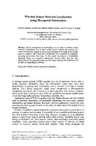
Figure 1.

BOL

Bearing Data Association

.. . sensor data N

BOL

DOAs batch N

target loc. 1

target loc. 2

.. . DOAs target Q

target loc. Q

BOL

Basic steps of the traditional localization approach

I. I NTRODUCTION Localization of multiple sources using passive sensor arrays is a fundamental task encountered in various fields like wireless communication, radar, sonar, seismology, and radio astronomy. Passive direction finding (DF) in contrast to active methods does not transmit known signals to illuminate the region of interest and processes reflected signals. That means passive DF methods deliver the signal direction of arrival (DOA) but no range information. Passive localization can be realized by multiple DF sensors or a single moving DF sensor. A moving platform is the preferable solution in many applications. The sensor is typically airborne, e.g. on an aircraft, a helicopter, or an unmanned aerial vehicle (UAV). Airborne DF sensors provide in comparison to ground located sensors a far-ranging signal acquisition because of the extended radio horizon. Mostly for localization issues, DF sensors are installed under the fuselage or in the wings of the airborne sensor platform. To localize emitters in impassable danger zones, preferably UAVs are used. Especially for small UAVs, the technological challenge lies in the integration of the several subsystems (e.g. energy supply, engine) and the payload in the smallest possible space. Due to the hard payload restrictions only compact DF sensors come into consideration. In this work, an airborne array sensor is considered observing multiple stationary sources and collecting multiple data batches. To localize the sources, the traditional localization approach depicted in Fig. 1 has been applied. Therein, at each time instance, a DF step has to performed in advance.

Aspects of the two-dimensional and three-dimensional bearings-only localization (BOL) problem examined in the literature include numerous estimation algorithms, estimation accuracy, and target observability [1]. Exemplarily, from the multitude of methods, two methods can be considered w.r.t. their estimation accuracy: the maximum likelihood estimator (MLE) and the extended Kalman filter (EKF), e.g., in modified polar coordinates [2]. As expected, the MLE offers accuracy benefits and requires a higher computational burden in comparison to the EKF. The MLE has proved to be particularly robust, and it has been shown to be asymptotically unbiased and efficient [3]. In this work, the MLE for the considered three-dimensional BOL problem will be used. Given those DOAs, a BOL algorithm can be used that can be geometrically interpreted as the intersection of the bearing lines. This technique is also referred to as triangulation. Generally, the bearing data association problem must be solved in order to employ BOL techniques. Tracking algorithms are known to lead to track loss whenever the DOAs of the targets cannot be resolved for a longer period of time. MHT is generally accepted as the preferred method for solving the observation-to-track association problem in modern multiplesource tracking systems [4]. MHT can deal with cases where the global nearest neighbor (GNN) approach or the joint probabilistic data association (JPDA) fail. However, in situations where the variances of the measurements are too large, even MHT is unable to partition the sensor data correctly. In our previous work, we proposed a direct position determination

(DPD) approach for a moving array sensor to solve the localization problem without explicitly computing bearings [5], [6]. In this way, the bearing data association problem can be circumvented. In [7], we used a probability hypothesis density (PHD) filter based on bearing measurements that also avoids the data association problem. However, in this paper, we assume an ideal bearing data association and focus on the sensor model and BOL techniques. Especially for small array sensors, biased bearing estimates may occur that depend on the signal DOA itself. A common problem is the usage of an idealistic sensor model, which cannot be observed in real applications. This approximation leads to a reduced localization performance. The main contribution of this paper is the incorporation of a realistic sensor model to the BOL approach to increase the localization accuracy. The paper is organized as follows: In Section II, we present the DOA accuracy for an ideal array sensor, a sensor with systematic errors, and a realistic array sensor. In Section III, we formulate the localization problem involving the sensor models. The CRBs on the estimation accuracy for the considered sensors are derived in Section IV. In Section V, we outline the considered localization techniques. Finally, in Section VI, we compare the accuracy of the considered array sensors in Monte Carlo simulations. The conclusions are given in Section VII. The following notations are used throughout this paper: (·)T and (·)H denote transpose and Hermitian transpose; In and 0n denote the n × n-dimensional identity and zero matrix; 0n denotes an n-dimensional zero vector, and E {·} denotes the expectation operation. II. D IRECTION F INDING ACCURACY In this Section, the DF problem using an antenna array is considered. Therefore, we define first of all the unit vector towards the signal DOA. For antenna arrays, it is natural to parameterize the unit vector by the antenna coordinates (also direction cosine or uv-coordinates) u = (u, v)T , u2 + v 2 ≤ 1, i.e.   u . v (1) e(u) = √ 1 − u2 − v 2 With the consideration of systematic bearing errors, angular coordinates are suitable to describe the DOA. E.g. for gimballed sensors, the DOA is almost always described by azimuth α and elevation ε. Also in this case, the DOA of the incident signal can be expressed in terms of the spherical angle ψ = (α, ε)T ∈ (−π, π] × [− π2 , π2 ] and the corresponding unit vector is given by (Fig. 2)   sin α cos ε e(ψ) = cos α cos ε . (2) sin ε

z

source

ε

sensor

v

u

α

y

x Figure 2. Relative vector given by antenna coordinates and spherical coordinates of the direction of arrival

A. Array Data Model It is important to establish a mathematical relationship between the array data and the source DOAs. The common array data model assumes that a set of Q narrowband signals with wavelength λ impinge as plane wave on an array sensor with M elements. Using complex envelope notation, the k-th sample, k = 1, ..., K, of the measurement vector zk ∈ CM can be expressed by the superimposed signals and the additional noise vector wk ∈ CM as zk =

Q X

a(eq ) sk,q + wk ,

(3)

q=1

where sk,q , k = 1, ..., K, q = 1, ..., Q, are the unknown source signal snapshots, and a(e) is referred to as the array transfer vector. In the literature, the array transfer vector is also named steering vector, array manifold vector, DOA vector, or array response vector. The array transfer vector expresses its complex response to a unit wavefront arriving from the DOA. For the considered far-field sources, the array response to a wavefront from the DOA is given by   2π T g1 (e) ej λ e d1   .. (4) a(e) =   . gM (e) ej

2π λ

eT dM

and depends on the unit vector e, the wavenumber 2π λ , the array element locations relative to a reference point commonly in the center of the array, and gm (e) ∈ C the element pattern of the m-th array element. The data model in (3) can be written more compactly as zk = A(e) sk + wk with e = (eT1 , ..., eTQ )T , A(e) = [a(e1 ), ..., a(eQ )] , sk = (sk,1 , ..., sk,Q )T .

(5)

B. Preprocessed Array Data The data covariance matrix (or spatial autocorrelation matrix) plays an important role in array signal processing, because it contains information about the array transfer vector and the signals. Since the array sensor collects a finite number of samples, the data covariance matrix can be estimated over K samples K 1 X zk zH (6) R= k . K k=1

Subspace-based DF techniques divide the data covariance matrix in a signal and noise subspace in order to estimate the DOAs. The subspaces are calculated by performing the following eigendecomposition of the data covariance matrix: H R = Us Λ s U H s + U w Λ w Uw ,

(7)

where the column vectors of Us ∈ CM ×Q and Uw ∈ CM ×M −Q are the eigenvectors spanning the signal and noise subspace of the covariance R, respectively, with the associated eigenvalues in decreasing order on the diagonals of Λs ∈ RQ×Q and Λw ∈ RM −Q×M −Q , respectively. To perform the eigendecomposition in (7), the number of source signals must be known or estimated, e.g. the number of source signals can be determined by a detection method [8]. C. Direction Finding In this work the deterministic data model is considered. In the deterministic signal model, each sample sk , k = 1, ..., K, is regarded to be fixed and unknown, i.e. each sample is an unknown deterministic parameter that needs to be estimated. Furthermore, the random vectors wk , k = 1, ..., K, are assumed to be zero-mean complex Gaussian [9], and temporally 2 and spatially uncorrelated, i.e. wk ∼ NC (wk ; 0M , σw IM ), 2 where σw denotes the receiver noise variance. In the literature numerous DF algorithms are described [10], e.g. in practice, the multiple signal classification (MUSIC) method is a widely-used method to solve the DF problem [11]. Using the subspace data, the normalized bearing function of the MUSIC method can be calculated by aH(ψ) a(ψ) . (8) H w Uw a(ψ) The DOA estimates can be obtained at the maximum locations of the bearing function. The MUSIC approach leads to a higher resolution capability in comparison to the conventional beamformer and tends to be power independent. Commonly, the array transfer vector in (8) is assumed to be ideal, i.e. gm (ψ) = 1, m = 1, ..., M . PMUSIC (ψ) =

aH(ψ) U

D. Sensor Models In practice, however, the array sensor cannot assumed to be ideal. In this subsection, we present the considered ideal array sensor, a sensor with systematic bearing errors as well as a realistic array sensor. Bearing errors may occur due to a mismatch between the array transfer vector in the array data model (4) and the DF method (8). The bearing errors are compared for the three cases.

1) Ideal Array Sensor: For an ideal array sensor, all element patterns have the same characteristic or are perfectly known, i.e. the element patterns gm (ψ), m = 1, ..., M , can be neglected in the array transfer vector. If correlations between the sources are neglected, the bearing error w.r.t. an individual source can be assumed as zero-mean Gaussian wψ ∼ N (02 , Cψ ) ,

(9)

where Cψ denotes the bearing covariance. In practice, the bearing covariance is unknown and needs to be estimated for localization purposes. For example, the bearing covariance for an uniform circular array (UCA) with M elements separated by the inter-element distance d can be approximated by [12], [13]  2   λ 1 1/ cos2 ε 0 , (10) Cψ = 0 1/ sin2 ε KM 3 SNR d 2 where SNR = s2 /σw is the single-element signal-to-noise ratio (SNR). Obviously, the bearing variances depend on the source SNR and the source elevation itself. 2) Sensor With Systematic Error: In praxis, several reasons can lead to systematic bearing errors, e.g. navigation errors such as errors in the own position or own attitude. A heading error for example immediately leads to an azimuth error. If the DF sensor and a navigation sensor are mounted on a platform, both sensors may be displaced in the attitude. Also biased bearing results can originate sensor calibration errors, e.g. electrical cable length differences between the array elements lead to bearing errors that are independent from the signal DOA. Therefore, the bearing errors can be assumed as

wψ ∼ N (β, Cψ )

(11)

where β = (βα , βε )T denotes the constant systematic bearing error w.r.t. the azimuth and elevation angle, respectively. 3) Realistic Array Sensor: The real antenna characteristic is influenced by element pattern differences and element coupling effects. These errors can be calibrated by an antenna measurement, i.e. the variations of the amplitude and phase response of each element, gm (ψ), m = 1, ..., M , are determined from the received signals zk , k = 1, ..., K. External and blind array calibration techniques are described in the literature. For example, the array can be calibrated by an external array measurement in an anechoic chamber, or the calibration of an airborne array is sensor is described in [14]. Through the array measurements, the element patterns can be deposited in the data model and can be considered in the used DF approach. In practice, however, the sensor errors cannot be compensated perfectly, e.g. due to the influence of the sensor platform. In this work, we consider a triangular array sensor with M = 3 elements and d ≈ λ2 . For this array, we measured the element characteristics in an anechoic chamber. This kind of antenna array measurements are advantageous to freespace measurements, because of less interferences of the plane wavefront due to ground reflections, scattering, and shadowing

sensor path

rN rn

z 4zn

x

4rn

r1

4yn

εn

y

4xn

αn Figure 3. Example of array element phase patterns in antenna coordinates without (left) and with (right) sensor platform

p Figure 4.

stationary source

Considered localization scenario with a single moving sensor

effects. For each element, the measurements are performed for several signal DOAs, frequencies and polarizations. To evaluate the platform influence, also measurements with the installed array sensor have been carried out. Transforming the near-field measurement results to the far-field, transforming the resulting data w.r.t. polarization, and neglecting the signal T phase 2π λ e dm , m = 1, ..., M , due to the array geometry, enables a suitable interpretation of the element patterns. For the case of co-polarization, Fig. 3 presents the measured element phase patterns in antenna coordinates. For the antenna under test, the phase patterns differ from element to element. Furthermore, the comparison of the patterns without and with the sensor platform in Fig. 3 shows significant differences. The variances of the phase error increases approximately by factor three due to the platform influence. Especially phase errors are objectionable, because the signal phase contains essential information about the source DOA. This leads to biased bearing results

If the sensor position r(tn ) (and the sensor attitude) are known, then the measurement function in (13) depends only on the target locations. With this, the localization problem is formulated as follows: Estimate the source location p from the collected bearing measurements

wψ ∼ N (β(ψ), Cψ ) ,

ˆ = ψ (p) + wψ,n , ψ n n

(12)

The measurement functions for the azimuth and elevation ψ n (p) = (αn , εn )T at measurement time tn , n = 1, ..., N , can be expressed as (Fig. 4) 4xn , 4yn 4zn εn (p) = arctan p , 4x2n + 4yn2

αn (p) = arctan

(13)

where 4xn , 4yn , and 4zn are the components of relative vector 4rn = p − r(tn ) . (14)

(15)

where the systematic error depends on the signal DOA itself.

where bearing error wψ,n , n = 1, ..., N , is related to the considered sensor models introduced in Section II-D.

III. L OCALIZATION P ROBLEM

IV. C RAM E´ R -R AO B OUND

The following three-dimensional scenario is considered, but the two-dimensional case can be treated completely analog to this case. For the sake of simplicity, we assume that the detection probability is equal to 1 and the false alarm rate is equal to 0. Let the array sensor collect N data batches at measurement times tn , n = 1, ..., N , and let assume that the sensor’s displacement during each measurement is negligible. The source DOAs can be calculated from the array data batches e.g. by using the MUSIC method presented in Section II-C. If the attitude of the sensor changes from observation to observation, then the bearing angles must be transformed into earth-fixed coordinates performing a suitable rotation by the platform heading, pitch, and roll angles. For the sake of simplicity, we assume a constant sensor attitude. Since we assume an ideal bearing data association, we consider the single source case. Thus, we omit the source index q for a better readability. The observer’s objective is to localize the targets from the collected array data batches.

For judging an estimation problem, it is important to know the maximum estimation accuracy that can be attained with the given measurements. The Cram´er-Rao bound (CRB) provides a lower bound on the estimation accuracy of any unbiased estimator, and its parameter dependencies reveal characteristic features of the estimation problem. A. Preliminaries ˆ (z) denote some unbiased estimate of the unknown Let p target parameters p based on the random measurements z. The covariance matrix C of the estimation error ˆ (z) 4p = p − p satisfies the multi-dimensional Cram´er-Rao inequality n o C = E 4p 4pT ≥ J−1 (p) ,

(16)

(17)

where the inequality is interpreted as stating that the matrix difference is positive semidefinite and J−1 (x) denotes the

CRB which is given by the inverse Fisher information matrix (FIM): ( T  ) ∂ ln L(p; z) ∂ ln L(p; z) . (18) J(p) = E ∂p ∂p If the estimator attains the CRB then it is called efficient. The log-likelihood function is given by N X

ˆ , ..., ψ ˆ ) = const − 1 wT C−1 wψ,n . (19) ln L(p; ψ 1 N 2 n=1 ψ,n ψ,n

C. Sensor With Systematic Errors In [17], the CRB on the location of a stationary target has been derived for the two-dimensional azimuth-only localization problem. Following these calculations, the corresponding CRB for the three-dimensional problem can be obtained by  −1 J(p) Jp,β −1 J (p, β) = , (22) JTp,β N I2 where J(p) is the FIM on the source location accuracy in (21) and " ∂α (p) #T N n X ∂p . (23) Jp,β = ∂εn (p) n=1

ˆ are random variables due In this log-likelihood function, ψ n to the random variables wψ,n , n = 1, ..., N . B. Ideal Array Sensor A few comments on the uniqueness condition are in order. Unambiguous localization results can be guaranteed, if the DOAs are identifiable for each observation (Q < M , d ≤ dmax ) [15], and there is not a constant line-of-sight between target and sensor [16]. For example, if the sensor moves exactly towards the relative vector, then the bearing lines can not be intersected. If a unique solution for the BOL problem exists, then one may be interested in the maximal estimation accuracy that can be achieved given the bearing measurements. Inserting the log-likelihood function in (18) and taking expectation, the FIM referring to the location results in J(p) =

T   N  X ∂ψ n (p) ∂ψ n (p) C−1 . ψ,n ∂p ∂p n=1

(20)

If azimuth and elevation are uncorrelated, the FIM can be calculated by [3]

J(p) =

N X

T   ∂αn (p) ∂αn (p) σ2 ∂p ∂p n=1 α,n  T   N X 1 ∂εn (p) ∂εn (p) + , σ2 ∂p ∂p n=1 ε,n 1



where the term N1 Jp,β JTp,β can be interpreted how much the estimation accuracy degrades caused by the circumstance that the sensor bias are part of the estimation problem. It is mentionable that the CRB is independent from the sensor bias β. V. L OCALIZATION A PPROACHES A standard solution of the localization problem stated in Section III consists of three steps (Fig. 1): the DF step (Section II-C), the bearing data association (tracking) step, and the BOL step. Before solving the BOL problem, the measurementto-track association problem must be solved by partitioning the measurements into sets of measurements belonging to the same source. The association problem can be solved for example by an MHT approach. The outcomes of this are multiple sets of DOAs that are called measurement tracks, where each of them corresponds to an individual target. The DOA track is given by the earth-fixed DOA estimates ˆ , ..., ψ ˆ . ψ 1

(21)

where the bearing variances are given by the diagonal elements of Cψ,n , and with ∂αn (p) 1 1 = (cos αn , − sin αn , 0) , ∂p 4rn cos εn ∂εn (p) 1 = (− sin αn sin εn , − cos αn sin εn , cos εn ) , ∂p 4rn where 4rn = |4rn | denotes the distance between sensor and source. Generally, the CRB depends on the DOA accuracy, the number of bearing measurements, and the target-observergeometry given by the relative vector in (14).

∂p

In the considered localization problem, the systematic sensor errors are nuisance parameters and only the source locations are desired parameters. The corresponding CRB on the source location accuracy can be calculated by applying the matrix inversion of a block-partitioned matrix to (22) −1  1 T , (24) J J J−1 (p) = J(p) − p,β p,β β N

N

A. Standard Bearings-only Localization To solve the BOL problem, the target location p must be estimated from the aforementioned DOA track. For an ideal array sensor, the BOL problem can be solved by maximizing the log-likelihood function in (19), and the cost function of the MLE has the following form: (N ) N X [ˆ αn − αn (p)]2 X [ˆ εn − εn (p)]2 ˆ = arg min p + , 2 2 p σα,n σε,n n=1 n=1 (25) where the expected DOAs αn (p) and εn (p) are given by the elements of measurement function (13) and the bearing variances are given by the diagonal elements of (10). For a proper choice of p the cost function (25) displays a global minimum. Therein, uncertain measurements make a small contribution to the optimization.

VI. S IMULATION R ESULTS

B. BOL With Systematic Bearing Errors (Bias-BOL) Now the BOL problem using a DF sensor that delivers biased DOAs is solved, where the target locations are of interest and the bias values are nuisance parameters. Taking the bias errors into account, the least squares estimator in (25) can be modified to (N X [ˆ αn − αn (p) − βα ]2 ˆ = arg min ˆ, β p 2 p,β σα,n n=1 ) N X [ˆ εn − εn (p) − βε ]2 + . (26) 2 σε,n n=1 In [18], a BOL approach has been proposed to improve the localization accuracy. The key idea is to process the bearing measurements that are related to their average value instead of processing the bearings themselves (Fig. 5). In this way, the bias parameters are not estimated explicitly. The cost function reads [18, Eq. C] (

ˆ = arg min p p

N X [(ˆ αn − α ¯ ) − (αn (p) − α ¯ (p))]2 2 σα,n n=1 ) N X [(ˆ εn − ε¯) − (εn (p) − ε¯(p))]2 , + 2 σε,n n=1

(27)

where the averaged bearing measurements and the averaged expected bearing measurements are given by N 1 X α ˆn , α ¯= N n=1

α ¯ (p) =

ε¯ =

ε¯(p) =

N 1 X αn (p) , N n=1 N 1 X εˆn , N n=1 N 1 X εn (p) . N n=1

p source location

α ˆ1 − α ¯

α ˆN − α ¯ α ¯

α ˆ1 r(t1 )

α ¯N r(tN )

observer path

Figure 5. Principle of the BOL approach based on biased bearing measurements

Simulations for the considered array sensors are carried out. The single-element single-source SNR is modeled by SNRn,q = SNR0,q /4rn,q , and we assume that SNR0,q = 5 dB, q = 1, ..., Q. In the considered scenario, we use a UCA composed of M elements separated by the inter-element space d = λ2 . The sensor fieldof-view is limited to the lower half sphere and suitable to localize ground-located emitters. At each measurement point the sensor collects an array data batch to calculate the source DOAs. Therefore, we use the MUSIC method presented in Section II-C. In the case of multiple sources, the bearing data association problem must be solved e.g. by an MHT approach. Anyway, since the signal frequency is identical, this quantity cannot be used as context information. All bearing measurements are subdivided in two DOA tracks each related to an individual source. In our simulations, we assume an ideal bearing data association. In the ground station (fusion center), the sensor-fixed DOAs are transformed to earth-fixed coordinates, and the emitter locations are computed by applying the standard BOL approach (25) and the Bias-BOL approach (27) to the DOA measurements. In our simulations, we use the simplex method of Nelder and Mead [19] to find the minima of the cost functions and we initialize every search with the true value. A. Ideal Array Sensor In this subsection, we illustrate the BOL principle. Within a simulation, an ideal UCA with M = 6 elements has been assumed collecting N = 20 data batches with K = 100 samples per batch. Moreover, Q = 2 sources are considered. Fig. 6 shows the experimental scenario setup with the sensor path (white line) and the measurement points (red dots). The emitters are located at the big red dots. For both DOA tracks, the azimuth bearings are pictured as two-dimensional bearing lines, while the estimated elevation angles that are necessary to estimate the emitter height are not depicted in Fig. 6(a,d). The source locations can be determined from the formed DOA tracks. Fig. 6(b,e) present the normalized BOL cost functions that correspond to the bearings depicted in Fig. 6(a,d). The magenta colored locations represent a low value of the cost function and the cyan colored locations a high value. The cost functions display a well-pronounced global minimum close to the true target location. Furthermore, the cost functions exhibit no further local minima. Monte Carlo simulations with 250 runs have been carried out to study the localization performance. The BOL approach in (25) is used to solve the localization problem. The estimation results of the Monte Carlo trials are plotted as white dots in Fig. 6(c,f). The projection on the xy-plane of corresponding concentration and Cram´er-Rao bound ellipses are depicted as white and red ellipses, respectively. The ellipses are typically oriented towards the sensor. For the ideal sensor the ellipses have a good consistency w.r.t. extension and orientation. It can

0.2

0.5

0.5

0.1

0

−0.5

∆ y [km] →

1

y [km] →

y [km] →

1

0

−0.5

−1 −1

−0.5

0 x [km] →

0.5

−1 −1

1

−0.1

−0.5

0 x [km] →

0.5

−0.2 −0.2

1

(b) BOL function, first source 0.2

0.5

0.5

0.1

−0.5

−1 −1

∆ y [km] →

1

0

0

−0.5

−0.5

0 x [km] →

0.5

1

−1 −1

(d) Bearing results, second source

0 ∆ x [km] →

0.1

0.2

0

−0.1

−0.5

0 x [km] →

0.5

1

(e) BOL function, second source Figure 6.

−0.1

(c) Scatter plot, first source

1

y [km] →

y [km] →

(a) Bearing results, first source

0

−0.2 −0.2

−0.1

0 ∆ x [km] →

0.1

0.2

(f) Scatter plot, second source

Simulation results for the BOL approach

be shown, that the employed BOL approach is asymptotically efficient with a growing number of measurements or increasing SNR. B. Comparison of the Array Sensors In this subsection, the localization performance of the array sensors introduced in II-D is compared. We consider a single source and and an UCA with M = 3 elements. For an ideal array sensor the root mean square error (RMSE) for both approaches is depicted in Fig. 7(a). It is mentioned that in this case also the Bias-BOL approach can be applied to estimate the unknown sensor bias βα = βε = 0◦ . The standard BOL as well as the Bias-BOL approach attain the corresponding CRB for growing number of measurements. This proofs that both BOL approaches are asymptotically efficient. Furthermore as expected, in this case the standard BOL approach offers a superior performance compared to the Bias-BOL approach. For a sensor with systematic bearing errors βα = 5◦ and βε = 10◦ , the corresponding RMSE is pictured in Fig. 7(b). Both approaches exhibit a decreased localization accuracy. As a consequence that the standard BOL approach does not account for the systematic bearing estimates, also the localization results are biased. For this reason, the standard BOL does not

approach the CRB while the Bias-BOL approach attains the corresponding CRB. In Fig. 7(c), the RMSE for realistic array sensor is presented. In this case, both standard BOL as well as Bias-BOL do not reach the CRB for a fixed bias, because the systematic bearing errors vary from measurement to measurement. This degrades the performance of the BOL approaches. Nevertheless, the bias variation can be approximated by a mean bias error that can be estimated by the Bias-BOL approach. This leads to a superior performance in comparison to the standard BOL approach. VII. C ONCLUSIONS In this paper, we derived the DF accuracy for an realistic array sensor based on the antenna measurements of a real array sensor. For the three-dimensional localization problem, we briefly reviewed the standard BOL approach and outlined a BOL approach that accounts for biased bearings without explicitly computing the systematic sensor errors. For the considered array sensor, the corresponding CRBs have been derived. In simulations, we compared the localization accuracy of the considered sensors. It has turned out that the standard BOL approach is the best choice for an ideal array sensor. For a sensor that delivers biased bearing results, the Bias-BOL ap-

proach considerably outperforms the standard BOL approach. Furthermore, this approach is asymptotically efficient for a growing number of measurements and has been also used for a realistic array sensor.

In fact, we have used this localization technique in real flight experiments with the real array sensor and obtained similar results. the presented Bias-BOL approach is not restricted to array sensors and can be also applied to any DF sensor that offers a similar behavior.

200

RMSE(pos) [m] →

R EFERENCES 150

100

50

0 0

5

10

15 n→

20

25

30

20

25

30

25

30

(a) Ideal array sensor

RMSE(pos) [m] →

200

150

100

50

0 0

5

10

15 n→

(b) Sensor with systematic bearing errors

RMSE(pos) [m] →

200

150

100

50

0 0

5

10

15 n→

20

(c) Realistic array sensor Figure 7. RMSE of the standard BOL approach (blue lines, crosses) and Bias-BOL approach (red lines, circles) compared with the CRB of an ideal sensor (black solid line) and a sensor with systematic errors (black dashed lines)

[1] K. Becker, “Target Motion Analysis (TMA),” in Advanced Signal Processing Handbook, S. Stergioulos, Ed. New York, NY: CRC Press, 2001, ch. 9, pp. 284–301. [2] V. J. Aidala and S. E. Hammel, “Utilization of modified polar coordinates for bearings-only tracking,” IEEE Trans. Automat. Contr., vol. 28, pp. 283–294, Mar. 1983. [3] S. C. Nardone, A. G. Lindgren, and K. F. Gong, “Fundamental properties and performance of conventional bearings-only target motion analysis,” IEEE Trans. on Automatic Control, vol. 29, pp. 775–787, Sep. 1984. [4] S. S. Blackman, “Multiple hypothesis tracking for multiple target tracking,” IEEE Aerosp. Electron. Syst. Mag, vol. 19, pp. 5–18, Jan. 2004. [5] M. Oispuu and U. Nickel, “Direct detection and position determination of multiple sources with intermittent emission,” Signal Processing, vol. 90, pp. 3056–3064, Dec. 2010. [6] B. Demissie, M. Oispuu, and E. Ruthotto, “Localization of multiple sources with a moving array using Subspace Data Fusion,” in Proc. ISIF 11th International Conference on Information Fusion, Cologne, Germany, Jul. 2008, pp. 131–137. [7] M. Schikora, D. Bender, D. Cremers, and W. Koch, “Passive multiobject localization and tracking using bearing data,” in Proc. ISIF 13th International Conference on Information Fusion, Edinburgh, UK, Jul. 2010. [8] M. Wax and T. Kailath, “Detection of signals by information theoretic criteria,” IEEE Trans. Acoust., Speech, Signal Processing, vol. 33, pp. 387–392, Apr. 1985. [9] A. van den Bos, “The multivariate complex normal distribution - a generalization,” IEEE Trans. Inform. Theory, vol. 41, pp. 537–539, Mar. 1995. [10] S. V. Schell and W. A. Gardner, “High-resolution direction finding,” in Handbook of Statistics, Signal Processing and its Applications, N. K. Bose and C. R. Rao, Eds. Elsevier, 1993, vol. 10, ch. 18, pp. 755–817. [11] R. O. Schmidt, “Multiple emitter location and signal parameter estimation,” IEEE Trans. Antennas Propagat., vol. 34, pp. 276–280, Mar. 1986. [12] S. F. Yau and Y. Bresler, “A compact Cram´er-Rao bound expression for parametric estimation of superimposed signals,” IEEE Trans. Signal Processing, vol. 40, pp. 1226–1230, May 1992. [13] P. Stoica and A. Nehorai, “MUSIC, Maximum Likelihood, and Cram´erRao bound,” IEEE Trans. Acoust., Speech, Signal Processing, vol. 37, pp. 720–741, May 1989. [14] H. S. Mir, J. D. Sahr, G. F. Hatke, and C. M. Keller, “Passive source localization using an airborne sensor array in the presence of manifold perturbations,” IEEE Trans. Signal Processing, vol. 55, pp. 2486–2496, Jun. 2007. [15] M. Wax and I. Ziskind, “On unique localization of multiple sources by passive sensor arrays,” IEEE Trans. Acoust., Speech, Signal Processing, vol. 37, pp. 996–1000, Jul. 1989. [16] K. Becker, “Simple linear theory approach to TMA observability,” IEEE Trans. Aerosp. Electron. Syst., vol. 29, pp. 575–578, Apr. 1993. [17] M. Gavish and E. Fogel, “Effect of bias on bearing-only target location,” IEEE Trans. Aerosp. Electron. Syst., vol. 26, pp. 22–26, Jul. 1990. [18] U. Steimel, “Some advantages of non-recursive TMA filters,” RTO SET Symposiom on Target Tracking and Sensor Data Fusion for Military Observation Systems, pp. 32.1–32.12, Oct. 2003. [19] J. A. Nelder and R. Mead, “A simplex method for function minimization,” Computer Journal, vol. 7, pp. 308–313, Jan. 1965.