Multiple Interactive Outputs in a Single Tree: An Empirical Investigation Edgar Galv´ an-L´opez1 and Katya Rodr´ıguez-V´azquez2 1
2
University of Essex, Colchester, CO4 3SQ, UK
[email protected] IIMAS-UNAM, Circuito Escolar s/n, Ciudad Universitaria Del. Coyoac´ an, M´exico, D.F. 04510, MEXICO
[email protected]
Abstract. This paper describes Multiple Interactive Outputs in a Single Tree (MIOST), a new form of Genetic Programming (GP). Our approach is based on two ideas. Firstly, we have taken inspiration from graph-GP representations. With this idea we decided to explore the possibility of representing programs as graphs with oriented links. Secondly, our individuals could have more than one output. This idea was inspired on the divide and conquer principle, a program is decomposed in subprograms, and so, we are expecting to make the original problem easier by breaking down a problem into two or more sub-problems. To verify the effectiveness of our approach, we have used several evolvable hardware problems of different complexity taken from the literature. Our results indicate that our approach has a better overall performance in terms of consistency to reach feasible solutions. Kerwords: Multiple Interactive Outputs in a Single Tree, Genetic Programming, Graph-GP representations.
1
Introduction
Genetic Programming (GP) [9] is a heuristic search technique, which has its inspiration from the theories of genetic inheritance and natural selection. This technique has been proved to be a suitable tool for solving problems in many applications. Usually, in GP programs are expressed as syntax trees. However, this form of GP has some limitations. So, some researchers have proposed different type of representations of GP. For example, Koza [10] proposed Automatically Defined Functions (ADFs). ADF is a function that is dynamically evolved during a run of a GP. The problem with this approach is discovering good ADFs. So, in order to discover if an ADF is good, GP has to spend computation time to discover with which parameters the ADF can be used properly. Angeline and Pollack [3] proposed a method called Evolutionary Module Acquisition (EMA). The idea of this method is to build and evolve modules (which are the reuse of code) during the evolution process. Because there is not a general method of identifying what portions of the individual should be
2
Edgar Galv´ an-L´ opez and Katya Rodr´ıguez-V´ azquez
compressed, the composition of each module is selected randomly. The same authors extended this work in [2]. The authors refer to the method as Genetic Library Builder (GLiB). Montana [13] proposed Strongly Typed Genetic Programming (STGP). He started from the definition of closure (which means that all elements take arguments of a single data type and return values of the same data type). The main characteristic of STGP is to build an individual as a parse tree and the data type of the nodes not necessarily should be the same type. Teller and Veloso [15] were one of the first researchers to use a graph-based GP. Their method, Parallel Algorithm Discovery and Orchestration (PADO), is a combination of GP and linear discriminator which was used to obtain a parallel classification programs for signals and images. Poli [14] proposed an approach called Parallel Distributed Genetic Programming (PDGP). Poli stated that PDGP can be considered as a generalisation of GP. However, PDGP can use more complex representations and evolve finite state automata, neural networks and more. PDGP is based on a graph-like representation for parallel programs which is manipulated by crossover and mutation operators and guarantee the syntactic correctness of the offsprings. Angeline [1] proposed a representation called Multiple Interacting Programs (MIPs). This representation is a generalization of a recurrent neural network that can model any type of dynamic system. Each program in a given set is unique and stored in the form of a parse tree. Using this technique an individual is virtually equivalent to a neural network where the computation performed at each unit is replaced with an independent evolved equation. Miller [12] proposed Cartesian Genetic Programming (CGP). This technique was called Cartesian in the sense that the method considers a grid of nodes that are addressed in a Cartesian coordinate system. In CGP the genotype is represented as a list of integers that are mapped to directed graphs rather than trees. Kantschik and Banzhaf [6] proposed a different representation of GP named Linear-Tree. The main idea was to give flexibility to a program to choose different execution paths for different inputs. In this method each program is represented as a tree. Later on, the same authors proposed a representation called LinearGraph [7]. They argued that graphs come one step nearer to the control flow of a hand written program. As it can be seen, different ideas have raised in GP to make it more efficient. The aims of this study are: (a) to study how GP behaves with and without the presence of graph-like structures, (b) to incorporate multiple outputs in individual’s structures, and, (c) to combine both properties (graph-like structures and multiple outputs in individual’s structures) and to see what the effects are. The paper is organised as follows. In the next section we describe our approach. Section 3 provides details on the experimental setup used and presents results. In section 4 we analyse the results found by our approach and in Section 5 we draw some conclusions.
Lecture Notes in Computer Science
3
Fig. 1. (a) GP-based representation of graphs without multiple outputs, (b) multiple outputs in a single tree (MOST) without links ,and, (c) multiple interactive outputs in a single tree (MIOST).
2
Approach
Our approach, which we have denominated Multiple Interactive Outputs in a Single Tree (MIOST), is based on two ideas. Firstly, we have taken inspiration from graph-GP representations. With this idea we decided to explore the possibility of representing programs as graphs with oriented links, see Figure 1(a). The idea was to replace a function node by other element that represents links which determine what’s need to be evaluated. We hope in this way to find parts of an individual that can be more useful in other part(s) of the same individual. Secondly, in our approach a program is represented as a tree as suggested by Koza with the main difference that a program could has more than one output, see Figure 1(b). Let us call this Multiple Outputs in a Single Tree (MOST). This idea was inspired on the Divide and Conquer principle, a program is decomposed in subprograms, and so, we are expecting to make the original problem easier by breaking down a problem into two or more sub-problems. In Figure 1(c), we can see a typical individual created with MIOST, which is the result of combining both ideas (graph-gp representation and MOST). 2.1
Output Set
Apart of considering function and terminal sets, as usual, we also consider another set which contain outputs. So, when we create an individual, we choose randomly from the set of outputs any of these and we eliminate it from this set. Once we have created an individual, we check if it contains all the outputs, if not we repeat the process until we have created a valid individual. It is worth mentioning that when we create an individual we do not specify which output will be in the root, so our approach has the power to place the most complex output in the root (results confirm this statement).
4
Edgar Galv´ an-L´ opez and Katya Rodr´ıguez-V´ azquez
2.2
P Symbol
The method proposed in this paper does not only allow having more than one output in a single tree but it also allows evolving graph-like structures. This is the result of using the p function symbol, which works as follows: – Once the individuals in the populations have been generated with its corresponding outputs, we use a probability to replace a function with a p symbol which is a function of arity 2 (This is not a restriction because p could be of any arity). – If an individual contains this p symbol, this will point to code somewhere in the program, so when p is executed, the subtree rooted at that node is ignored. – If p symbol points to a function symbol, the p symbol effectively represents the sub-tree rooted at that function. – If p symbol points to a terminal symbol, the p symbol simply represents that node. 2.3
Genetic Operators
The crossover operator used in MIOST works as usual but an important difference is that, if the sub-tree swapped contained a p symbol, the p symbol’s pointer is not changed3 . Another difference is that once we have created our initial population, we classify each node of each individual in order to know which nodes can be used to apply crossover. With this we assure that an individual will contain the number of outputs that must contain. Of course, this classification is only applied when the individual has more than one output. The mutation operator is applied as usual on a per node basis. The only restriction is that a p symbol is not allowed to be mutated. 2.4
Fitness Function
To test the effectiveness of our approach, we have used several evolvable hardware problems of different complexity taken from the literature. The fitness function works in two stages: at the beginning of the search, the fitness of a genotype is the number of correct output bits (raw fitness). Once the fitness has reached the maximum number of correct outputs bits, we try to optimize the circuits by giving a higher fitness to an individual with shorter encodings. 2.5
Features
The approach detailed above has interesting features. For instance, the presence of p symbols in our representation, assure us that there are inactive code in the 3
There is an exception to this rule: we prevent a p symbol from referring to a sub-tree that contains the same p since this would lead to an infinite loop. We do this by reassigning the position to which the p in question is pointing to.
Lecture Notes in Computer Science Table 1. Truth table of the second example. A 0 0 0 0 0 0 0 0 1 1 1 1 1 1 1 1
B 0 0 0 0 1 1 1 1 0 0 0 0 1 1 1 1
C 0 0 1 1 0 0 1 1 0 0 1 1 0 0 1 1
D 0 1 0 1 0 1 0 1 0 1 0 1 0 1 0 1
O1 1 1 1 0 1 1 0 0 1 0 0 0 0 0 0 0
O2 0 0 0 0 0 0 0 0 0 0 0 1 0 0 1 1
5
Table 2. Truth table of the third example. A 0 0 0 0 0 0 0 0 0 0 0 0 0 0 0 0
B 0 0 0 0 0 0 0 0 1 1 1 1 1 1 1 1
C 0 0 0 0 1 1 1 1 0 0 0 0 1 1 1 1
D 0 0 1 1 0 0 1 1 0 0 1 1 0 0 1 1
E 0 1 0 1 0 1 0 1 0 1 0 1 0 1 0 1
O1 1 1 1 1 1 1 1 1 1 1 1 1 1 1 1 1
O2 1 0 1 0 1 0 1 1 1 0 1 0 1 0 1 1
O3 0 0 0 0 1 1 0 0 0 0 0 0 1 1 0 0
A 1 1 1 1 1 1 1 1 1 1 1 1 1 1 1 1
B 0 0 0 0 0 0 0 0 1 1 1 1 1 1 1 1
C 0 0 0 0 1 1 1 1 0 0 0 0 1 1 1 1
D 0 0 1 1 0 0 1 1 0 0 1 1 0 0 1 1
E 0 1 0 1 0 1 0 1 0 1 0 1 0 1 0 1
O1 0 0 0 0 0 0 0 0 0 0 0 0 1 1 1 1
O2 1 0 1 0 1 0 1 1 1 0 1 0 1 0 1 1
O3 0 0 0 0 1 1 0 0 0 0 0 0 1 1 0 0
individual. This has two advantages: when a mutation takes place in inactive code there is no need to evaluate an individual since there is a change at genotype level but not at phenotype level, and, it allows to study neutrality [8] which is an area of controversial debate on Evolutionary Computation (EC) systems.
3
Experiments
As stated earlier, our approach is based on two ideas. So, for the first problem we will test the first idea. That is, we have used only the graph-like presentation (Figure 1(a)). We used only mutation operator and we have defined different mutation and p rates. For this example, we used the following set of gates {AND,OR,NOT }. As a consequence of the results obtained from the first example, we have decided to test MIOST on three different hardware problems with different degrees of complexity. Our results were compared with those obtained by MGA [4], EAPSO [16], EBPSO [11], BPSO [11], EGP [5] and MOST. For these examples, we used the following set of gates {AND, OR, XOR, NOT}. After a series of preliminary experiments we have decided to use crossover rate of 0.7%, mutation rate of 0.02%, and p rate of 0.08% for all examples except for example 1 where we have defined different values. To make a fair comparison with the previous methods, we used the same number of generations and population size. Runs were stopped when the maximum number of generations was reached. For all examples, we performed 20 independent runs.
6
Edgar Galv´ an-L´ opez and Katya Rodr´ıguez-V´ azquez Table 3. Truth table of the fourth example. A 0 0 0 0 0 0 0 0 1 1 1 1 1 1 1 1
3.1
B 0 0 0 0 1 1 1 1 0 0 0 0 1 1 1 1
C 0 0 1 1 0 0 1 1 0 0 1 1 0 0 1 1
D 0 1 0 1 0 1 0 1 0 1 0 1 0 1 0 1
O1 1 0 0 0 0 1 0 0 0 0 1 0 0 0 0 1
O2 0 1 1 1 0 0 1 1 0 0 0 1 0 0 0 0
O3 0 0 0 0 1 0 0 0 1 1 0 0 1 1 1 0
Example 1
For our first example, we have used the well-known 6-bit Multiplexer Boolean function to verify the idea of graph-like representation (without multiple outputs). For our first example we have used Population Size (PS) = 200, and Maximum Number of Generations (MNG) = 400, p = {0.01, 0.02, 0.03} and mut = {0.02, 0.03, 0.04}. In Table 4 we can see the results found by the gp-graph representation. In this table we present the percentage of feasible circuits (success rate) and the average number of generations that were necessary to reach the feasible zone4 . As can be seen, regardless the value of p, the best results were found when mutation rate = 0.02. Does this mean that the presence of p is useless on the evolutionary process? To answer this question, we remove p from the evolutionary search and keep the same mutation rates. The success rates for mutation rates 0.02, 0.03 and 0.4 were 65%, 75%, 45%, respectively. From these results, it seems to be that the addition of p symbols to the individuals’ structures aid the evolutionary search. 3.2
Example 2
For our second example we have used the truth table shown in Table 1. The parameters used in this example are the following: PS = 380 and the MNG = 525 (i.e., a total of 199,500 fitness function evaluations). The same values parameters 4
The feasible zone is the area of the search space containing circuits that match all the outputs of the problem’s truth table.
Lecture Notes in Computer Science
7
Table 4. Results found using the gp-graph representation on the 6-bits Multiplexer problem. P and mutation rates are shown in the first and second row, respectively. Feasible Circuits (Success Rate) and Average of Generations (this refers to the average number of generations that were necessary to reach the feasible zone) are shown in the last two rows, respectively. % p = 0.01 % p = 0.02 % p = 0.03 %mut= %mut= %mut= 0.02 0.03 0.04 0.02 0.03 0.04 0.02 0.03 0.04 % of feasible circuits 100% 90% 70% 75% 65% 50% 85% 85% 45% Average of generations 80.6 155.66 138.62 91.46 136.66 141.5 122.7 109.64 179.5 Table 5. Comparison of results between BPSO, EAPSO, EBPSO, MGA, EGP, MOST and MIOST on the second example.
BPSO EAPSO EBPSO MGA EGP MOST MIOST
Feasible circuits Avg. # of gates Avg. of gen. 95% 10.05 70% 13.45 100% 7.75 75% 13.4 55% 9.7 122.9 85% 14.98 53.29 100% 12.9 109.55
were used by EGP and MOST. BPSO, EAPSO and EBPSO performed 200,000 fitness function evaluations, while MGA performed 201,300. As we can see in Table 5, the only algorithms able to converge to the feasible region in 100% of the runs were EBPSO and MIOST. 3.3
Example 3
For our third example we have used the truth table shown in Table 2 (Notice that this truth table was split in two due to space limitations). The parameters used in this example are the following: PS = 1,200 and the MNG = 832 (i.e., a Table 6. Comparison of results between BPSO, EAPSO, EBPSO, MGA, GP, EGP, MOST and MIOST on the third example.
BPSO EAPSO EBPSO MGA EGP MOST MIOST
Feasible circuits Avg. # of gates Avg. of gen. 25% 23.95 50% 18.65 45% 20.1 65% 17.05 60% 9.66 149.5 50% 11.3 94.5 75% 11.6 104.67
8
Edgar Galv´ an-L´ opez and Katya Rodr´ıguez-V´ azquez
Table 7. Comparison of results between BPSO, EAPSO, EBPSO, MGA, GP, EGP, MOST and MIOST on the fourth example.
BPSO EAPSO EBPSO MGA EGP MOST MIOST
Feasible circuits Avg. # of gates Avg. of gen. 30% 10% 20 234.16 35% 22.16 277.363
total of 998,400 fitness function evaluations). The same values parameters were used by EGP and by MOST. BPSO, EAPSO and EBPSO performed 1,000,000 fitness function evaluations, while MGA performed 1,101,040. As we can see in Table 6, MIOST is the algorithm which has the highest percentage of feasible solutions reached (75%). 3.4
Example 4
For our fourth and last example (also know as Katz circuit) we have used the truth table shown in Table 3. The parameters used in this example are the following: PS = 880 and the MNG = 4,000 (i.e., a total of 3,520,000 fitness function evaluations). The same values parameters were used by EGP and MOST. As we can see in Table 7, MIOST is the algorithm which has the highest percentage of feasible solutions reached (35%).
4
Analysis
For analysis purposes, we have conducted our experiments in the following way: 1. Firstly, we have allowed to the individuals having p symbols in their representation and in this way, we have been able to have a gp-graph representation, 2. Secondly, we have used MOST which is form of GP that has allowed us to define multiple outputs in each individual and 3. Thirdly, we have used MIOST, which is a combination of the previous ones. In other words, the individuals in MIOST have p symbols in their structures and multiple outputs. Let us focus our attention on the first example. In this example we decided to test an individual partially created with our approach. That is, we have specified to build an individual with links without multiple outputs. To verify how good this idea is, we used only mutation operator in this example. The presence of p symbols in individuals’ structures is necessary to improve performance on the evolutionary process (results confirm this statement). However, when p was not present in any of our individuals, the performance of the GP was worst.
Lecture Notes in Computer Science
9
From the results obtained in the first example, we decided to incorporate this idea to the representation where an individual can have more than one output (MOST). This combination of ideas gave us as a result MIOST representation and it was tested on the last three examples which are more complex problems. Our results indicate that MIOST has a better overall performance in terms of consistency to reach feasible solutions in all the examples. Let us analyse the results we have found with our approach for the last three examples. For the example 2, the average number of generations to solve the problem using MIOST is 109.55, while in MOST the average number of generations is 53.29. Similar situation is observed in examples 3 and 4, where the average number of generations to solve the problem using MIOST is 104.67 and 277.363, while in MOST the average number of generations is 94.5 and 234.16, respectively. As can be seen, the presence of p symbols in MIOST seems to require more generations to find the feasible circuit. This can be explained, if we consider that mutations could take place on inactive code that does not produce any change at phenotype level. On the other hand, this inactive code can have a role where partial solutions are protected against disrupted mutations. However, further analysis needs to be done to give final conclusions.
5
Conclusions
In this paper we have presented MIOST which is a new form of genetic programming which has two main features: (a) it allows to represent programs as graphs with oriented links (graph-GP representation) and (b) a program can have more than one output. We have used four evolvable hardware problems of different complexity to carry out our experiments with the proposed approach. Firstly, we used MOST to see how good the idea was by using only multiple outputs in our individuals. Once we saw that this gave us good results, we tested our approach (MIOST) which incorporates the idea of gp-graph representation in the presence of p symbols in individuals’ structure. Our results indicate that MIOST has a better overall performance in terms of consistency in reaching feasible solutions. However, our approach was not able to improve previously published results in terms of number of gates. This is due two reasons (a) our approach is not an optimization technique and (b) our approach has the restriction that one or more outputs depend on the solution of one or more outputs. This can be seen easily by analyzing Figure 1(c).
Acknowledgments The first author thanks to CONACyT for support to pursue graduate studies at University of Essex. The second author gratefully acknowledges support from CONACyT through project 40602-A. The authors would like to thank the anonymous reviewers for their valuable comments.
10
Edgar Galv´ an-L´ opez and Katya Rodr´ıguez-V´ azquez
References 1. P. J. Angeline. Multiple interacting programs: A representation for evolving complex behaviors. Cybernetics and Systems, 29(8):779–806, Nov. 1998. 2. P. J. Angeline and J. B. Pollack. Coevolving high-level representations. July Technical report 92-PA-COEVOLVE, Laboratory for Artificial Intelligence. The Ohio State University, 1993. 3. P. J. Angeline and J. B. Pollack. Evolutionary module acquisition. In D. Fogel and W. Atmar, editors, Proceedings of the Second Annual Conference on Evolutionary Programming, pages 154–163, La Jolla, CA, USA, 25-26 Feb. 1993. 4. C. Coello and A. Aguirre. Design of combinational logic circuits through and evolutionary multiobjective optimization approach. In Artificial Intelligence for Engineering, Design, Analysis and Manufacture, volume 16, pages 39–53, January. 2002. 5. E. Galvan-Lopez, R. Poli, and C. C. Coello. Reusing code in genetic programming. In M. Keijzer, U.-M. O’Reilly, S. M. Lucas, E. Costa, and T. Soule, editors, Genetic Programming 7th European Conference, EuroGP 2004, Proceedings, volume 3003 of LNCS, pages 359–368, Coimbra, Portugal, 5-7 Apr. 2004. Springer-Verlag. 6. W. Kantschik and W. Banzhaf. Linear-tree GP and its comparison with other GP structures. In J. F. M. et al., editor, Proceedings of EuroGP’2001, volume 2038 of LNCS, pages 302–312, Lake Como, Italy, 18-20 Apr. 2001. Springer-Verlag. 7. W. Kantschik and W. Banzhaf. Linear-graph GP—A new GP structure. In J. A. Foster, E. Lutton, J. Miller, C. Ryan, and A. G. B. Tettamanzi, editors, Genetic Programming, Proceedings of the 5th European Conference, EuroGP 2002, volume 2278 of LNCS, pages 83–92, Kinsale, Ireland, 3-5 Apr. 2002. Springer-Verlag. 8. M. Kimura. Evolutionary rate at the molecular level. In Nature, volume 217, pages 624–626, 1968. 9. J. R. Koza. Genetic Programming: On the Programming of Computers by Means of Natural Selection. The MIT Press, Cambridge, Massachusetts, 1992. 10. J. R. Koza. Genetic Programming II: Automatic Discovery of Reusable Programs. The MIT Press, Cambridge, Massachusetts, 1994. 11. E. H. Luna, C. C. Coello, and A. H. Aguirre. On the use of a population-based particle swarm optimizer to design combinational logic circuits. In R. S. Z. et al., editor, Proceedings of the 2004 NASA/DoD Conference on Evolvable Hardware, pages 183–190, Los Alamitos, California, June 2004. IEEE Computer Society. 12. J. F. Miller and P. Thomson. Cartesian genetic programming. In R. Poli, W. Banzhaf, W. B. Langdon, J. F. Miller, P. Nordin, and T. C. Fogarty, editors, Genetic Programming, Proceedings of EuroGP’2000, volume 1802 of LNCS, pages 121–132, Edinburgh, 15-16 Apr. 2000. Springer-Verlag. 13. D. J. Montana. Strongly typed genetic programming. BBN Technical Report #7866, Bolt Beranek and Newman, Cambridge, MA 02138, USA, 7 May 1993. 14. R. Poli. Parallel distributed genetic programming. In D. Corne, M. Dorigo, and F. Glover, editors, New Ideas in Optimisation. McGraw-Hill, 1999. 15. A. Teller and M. Veloso. PADO: Learning tree structured algorithms for orchestration into an object recognition system. Technical Report CMU-CS-95-101, Department of CS, Carnegie Mellon University, Pittsburgh, PA, USA, 1995. 16. X. Xu, R. C. Eberhart, and Y. Shi. Swarm intelligence for permutation optimization: A case study on n-queens problem. In Proceedings of the IEEE Swarm Intelligence Symposium 2003, pages 243–246, Indianapolis, Indiana, USA, 2003.